Phase Transitions Between Topologically Distinct Gapped Phases in Isotropic Spin Ladders

Abstract

We consider various two-leg ladder models exhibiting gapped phases. All of these phases have short-ranged valence bond ground states, and they all exhibit string order. However, we show that short-ranged valence bond ground states divide into two topologically distinct classes, and as a consequence, there exist two topologically distinct types of string order. Therefore, not all gapped phases belong to the same universality class. We show that phase transitions occur when we interpolate between models belonging to different topological classes, and we study the nature of these transitions.

I Introduction

Even though the spectrum of the spin-1/2 Heisenberg chain was obtained by Bethe[1] almost seventy years ago using his famous Ansatz, low-dimensional spin systems are still a strong area of activity, full of surprises and puzzles. A major source of this activity was Haldane’s conjecture,[2] which predicted that isotropic antiferromagnetic Heisenberg chains with integer spin have a gapped spectrum, while chains with half-integer spin have a gapless spectrum. There has been considerable theoretical and experimental evidence in support of Haldane’s conjecture; it is probably appropriate to call it a theorem, despite the lack of a rigorous mathematical proof.[3] Incidentally, the gapped phase in integer spin Heisenberg chains has come to be known as the Haldane phase.

A breakthrough in understanding the nature of the Haldane phase came when it was realized that one can go without a phase transition from the spin-1 Heisenberg chain to the AKLT model,[4] where the ground state is made up solely of nearest neighbor valence bonds. The Haldane gap is thus related to the energy needed to break short-ranged valence bonds.

FIG. 1.: (a) Typical configuration of the spin-1 chain. (b) Néel order after removing all sites with $S^{\alpha}_{i}=0$.

Another important step was when den Nijs and Rommelse identified a hidden order in the Haldane phase of the spin-1 chain.[5] They showed that although the sites with $S^{\alpha}_{i}=1,0,-1$ are not well ordered in position, their sequence is ordered in the way shown schematically in Fig. 1. That is, if we remove all sites with $S^{\alpha}_{i}=0$, the remaining sites have Néel order. The order parameter which reveals this hidden order is the non-local string order parameter

$${\cal O}^{\alpha}=-\lim_{|i-j|\rightarrow\infty}\left\langle S^{\alpha}_{i}\exp\left(i\pi\sum_{l=i+1}^{j-1}S^{\alpha}_{l}\right)S^{\alpha}_{j}\right\rangle\,,$$ (1)

where $S^{\alpha}_{i}$ is the spin-1 operator at site $i$, and $\alpha=x,y,z$.

A further impetus for the study of low-dimensional spin systems was given recently by the discovery of spin-ladder materials.[6] Since the spin-1/2 Heisenberg chain has a gapless excitation spectrum with spin-spin correlation functions exhibiting power-law behavior, it initially came as a surprise when it was found that the two-leg ladder had a gapped spectrum with exponentially decaying spin-spin correlations,[7] while the gapless spectrum survived in the three-leg ladder. Thus ladders could have a gapped or gapless spectrum, depending on the number of legs. More specifically, Heisenberg ladders with an even number of legs have a gapped spectrum, while ladders with an odd number of legs have a gapless spectrum.

The appearance of a gapped spectrum for even-legged ladders and a gapless spectrum for odd-legged ladders is highly reminiscent of Haldane’s conjecture for spin chains. Therefore, a natural question arises: Is the gapped phase in spin ladders related to the Haldane phase in spin chains? In particular, does the gapped phase exhibit string order? For the rest of the paper, we will restrict our discussion to the two-leg ladder.

For the case of ferromagnetic interchain coupling, it is clear that the two-leg ladder can be equivalent to the spin-1 chain, with the two spins on a rung forming an effective $S=1$. Such a phase is directly related to the Haldane phase, and the system has string order. Similarly, if the interchain coupling is antiferromagnetic and along plaquette diagonals, when the interchain coupling is equal to the coupling along the chains, the model is in fact the composite spin representation of the spin-1 chain; thus, the gapped phase is equivalent to the Haldane phase. (See Sec. II for a more detailed discussion of the composite spin representation.) Besides the gap, these models exhibit another characteristic feature of the Haldane phase. Namely, the ground state is unique if periodic boundary conditions are used, but it is four-fold degenerate for open boundary conditions.

A gap appears in the excitation spectrum of spin ladders for other types of interchain coupling as well, namely for antiferromagnetic coupling along the rungs or ferromagnetic coupling along plaquette diagonals. Whether these gapped phases are related to the Haldane phase is much less obvious. For example, for antiferromagnetic interchain coupling along the rungs, the zeroth order picture is given by studying the limit in which the interchain coupling is much larger than the coupling along the chains (i.e., $J_{\perp}\gg J$). In this limit, the ground state is well described by a product of rung singlets, with an energy gap $\sim J_{\perp}$ to break a singlet and form a triplet excitation. Here, the ground state is unique, irrespective of whether open or periodic boundary conditions are used. Nevertheless, as was demostrated by White,[8] the antiferromagnetic ladder can be transformed continuously to a model (seemingly) equivalent to the composite spin representation of the spin-1 chain by switching on an irrelevant further neighbor coupling. Consequently, the antiferromagnetic ladder is also related, in some way, to the Haldane phase and has string order.[8, 9]

There are also other types of ladders exhibiting spin gapped phases, so the question of string order in ladders and the relationship of the gapped phases to the Haldane phase becomes even more interesting. In particular, the spin-1/2 chain with second neighbor coupling is often represented as a two-leg zig-zag ladder.[10] For a particular value of the couplings, the so-called Majumdar-Ghosh point,[11] the ground state is known exactly. It is doubly degenerate and the excitation spectrum is gapped; each ground state consists of a sequence of independent singlets. However, it was shown that the Majumdar-Ghosh ground state has perfect string order.[12] It has also been shown[13] that the Majumdar-Ghosh model can be smoothly connected to the ladder with strong ferromagnetic rung coupling, which is equivalent to a spin-1 chain, without a phase transition.

Since the ground state of the Majumdar-Ghosh model consists of decoupled singlets, similar to the ground state of the ladder with strong antiferromagnetic coupling along the rungs, one might get the impression that all spin-gapped phases can be smoothly connected to each other. By this we mean that one can go from one model to another by continuously varying the model parameters without undergoing a phase transition. In this paper, we show that the gapped phases in isotropic two-leg spin ladders divide into two topologically distinct classes. This implies that phase transitions must necessarily occur if we try to interpolate between models belonging to different topological classes. Although not all gapped phases are directly equivalent to the Haldane phase of the spin-1 chain, all possess some kind of string order.

The rest of the paper is organized as follows. In Sec. II we introduce the spin ladder models that we will consider, and we recapitulate briefly what is known about these models. In Sec. III we discuss the relationship between valence bond states and string order, and also the possibility of phase transitions between spin models with topologically different string order. A bosonization treatment of the various models is presented in Sec. IV, and a discussion of the results obtained is given in Sec. V. Finally, Sec. VI gives a summary of our results and an outlook for future work.

II The Models

We begin with two antiferromagnetic spin-1/2 Heisenberg chains with the Hamiltonian

$${\cal H}_{0}=J\sum_{i=1}^{N}\left(\vec{S}_{i,1}\cdot\vec{S}_{i+1,1}+\vec{S}_{i,2}\cdot\vec{S}_{i+1,2}\right),$$ (2)

where $\vec{S}_{i,1}$ ($\vec{S}_{i,2}$) is the spin operator at site $i$ on chain 1 (chain 2). We will consider various forms for the interchain coupling.

The interchain coupling

$${\cal H}_{1}=J_{1}\sum_{i=1}^{N}\vec{S}_{i,1}\cdot\vec{S}_{i,2}$$ (3)

describes the usual rung coupling along the legs of the ladder. This type of ladder is shown in Fig. 2. (We will simply refer to this ladder model as a ladder.)

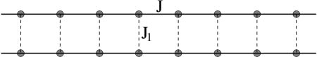
FIG. 2.: The usual two-leg ladder.

When $J_{1}$ is strongly ferromagnetic ($J_{1}<0$ and $|J_{1}|\gg J$) the two spins on the rung form a triplet, the singlet being much higher in energy. In this limit, the ladder behaves like a spin-1 chain, and hence the spectrum is gapped. However, it has been shown[14] that a gap is generated by an arbitrarily small ferromagnetic coupling. Therefore, it appears that weak and strong ferromagnetic coupling are continuously related.

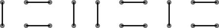
FIG. 3.: A typical configuration in the RVB state of the antiferromagnetic ladder. Solid lines represent singlet bonds.

When $J_{1}$ is strongly antiferromagnetic ($J_{1}>0$ and $J_{1}\gg J$), the ground state is essentially a product of rung singlets with a gap to magnon excitations. When $J_{1}=J$, it was shown that the ground state is well described by a nearest neighbor resonating valence bond (RVB) state and has a gap to the excited states.[15] A typical configuration of the RVB state is shown in Fig. 3. Similar to the ferromagnetic case, it has been shown[16, 17] that the spectrum is gapped for arbitrarily small antiferromagnetic interchain coupling. Therefore, weak and strong antiferromagnetic coupling also seem to be continuously related.

We will also consider a ladder in which the interchain coupling is along plaquette diagonals

$${\cal H}_{2}=J_{2}\sum_{i=1}^{N}\left[\vec{S}_{i,1}\cdot\vec{S}_{i+1,2}+\vec{S}_{i,2}\cdot\vec{S}_{i+1,1}\right].$$ (4)

Together with ${\cal H}_{0}$ this gives the ladder shown in Fig. 4. (We will refer to this ladder as a diagonal ladder.)

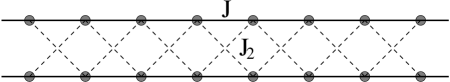
FIG. 4.: The diagonal ladder model.

For $J_{2}=J$, this model is in fact the composite spin representation of a spin-1 chain. More precisely, by starting with the Hamiltonian of a spin-1 chain

$\displaystyle{\cal H}=J\sum_{i=1}^{N}\vec{S}_{i}\cdot\vec{S}_{i+1}\,,$

and representing the spin-1 operator on site $i$ as the sum of two spin-1/2 operators, $\vec{S}_{i}=\vec{S}_{i,1}+\vec{S}_{i,2}$, we find

$\displaystyle{\cal H}={\cal H}_{0}+{\cal H}_{2}\,,$

with $J_{2}=J$. In the composite spin representation, the total spin of each rung commutes with the Hamiltonian, so the eigenstates can all be classified by the total spin on each rung. The set of eigenstates with only triplets on all of the rungs corresponds to the spectrum of the spin-1 Heisenberg chain. Hence, the low energy spectrum of the composite spin representation is identical to that of a spin-1 chain.[18] The ground state of this model is well described by the AKLT state, [4] a typical configuration of which is shown in Fig. 5. Here again, it has been shown[19] that a gap appears for arbitrarily small $J_{2}>0$. It has also been shown[19] that the spectrum is gapped for $J_{2}<0$; in fact, the gap is generated for arbitrarily small $J_{2}<0$. Therefore, it appears that weak and intermediate coupling are continuously related for both $J_{2}>0$ and $J_{2}<0$, however the gap vanishes at $J_{2}=0$.

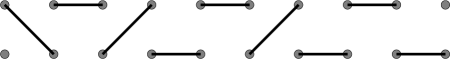
FIG. 5.: A typical configuration in the AKLT state of the diagonal ladder. Solid lines represent singlet bonds.

As one can see from Fig. 5, for a finite system there are effectively free spin-1/2’s at the ends of the ladder, which are responsible for a four-fold degenerate ground state. When periodic boundary conditions are used, all of the spins are bound into singlets and the ground state is unique.

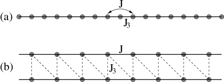
FIG. 6.: The zig-zag ladder shown as (a) a chain with first and second neighbor interactions (b) a ladder.

Finally, we will consider an interchain coupling similar to ${\cal H}_{2}$, but with only one of the diagonal couplings

$${\cal H}_{3}=J_{3}\sum_{i=1}^{N}\vec{S}_{i+1,1}\cdot\vec{S}_{i,2}.$$ (5)

We consider such an interchain coupling because, for $J_{1}=J_{3}$, we can write this model as a spin-1/2 Heisenberg chain with first and second neighbor interactions

$${\cal H} = {\cal H}_{0}+{\cal H}_{1}+{\cal H}_{3}$$

$$= J_{3}\sum_{i=1}^{2N}\vec{S}_{i}\cdot\vec{S}_{i+1}+J\sum_{i=1}^{2N}\vec{S}_{i}\cdot\vec{S}_{i+2}$$

(See Fig. 6). (We will refer to this type of ladder [for $J_{1}=J_{3}$] as a zig-zag ladder.)

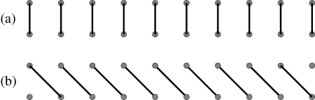
FIG. 7.: The two degenerate ground states of the zig-zag ladder at the Majumdar-Ghosh point. Solid lines represent singlet bonds.

The zig-zag ladder is known[10] to have a quantum phase transition from critical, gapless behavior to a spontaneously dimerized gapped phase as $J$ increases at $J=0.241J_{3}$. Moreover, at the special Majumdar-Ghosh point[11] ($J=0.5J_{3}$), the ground state is known exactly. It is two-fold degenerate in the thermodynamic limit, and each of the ground states is a sequence of decoupled singlets, as shown in Fig. 7. In fact, it has been shown that for $0.241<J/J_{3}<\infty$, the zig-zag ladder is gapped and has dimer order.[10, 20] Therefore, it appears that the entire range $0.241<J/J_{3}<\infty$ is continuously related to the Majumdar-Ghosh point.

III Valence Bond States and String Order

As previously mentioned, all of our models have short-ranged (SR) valence bond (VB) ground states, and all of our models exhibit string order. In this section, we will argue that there are two topologically distinct types of string order and that these two types of string order are intimately related to the VB structure.

In general, any singlet state of an SU(2) symmetric model can be represented in terms of VB’s. The SR-VB ground states of gapped spin liquids are, in the typical case, a linear combination of a large number of VB configurations, in which the probability to find a longer ranged VB is exponentially small. The gap in the spectrum is related to the finite energy needed to break a VB. On the other hand, systems with a gapless spectrum necessarily contain longer VB’s as well.

In order to see the connection between the VB structure and string order, we first consider the diagonal ladder with $J_{2}=J$. The ground state is well described by the RVB picture of the AKLT state. A typical configuration was shown in Fig. 5. One particular spin configuration of Fig. 5 is shown in Fig. 8(a). Suppose we add the $z$ component of the spins on the same rung, as shown in Fig. 8(b). The total $S^{z}_{i}$ can take on the values $1,0,-1$. Considering this sequence, if we remove all sites with $S^{z}_{i}=0$, the remaining sites have Néel order (i.e. there is string order). If, on the other hand, the $z$ components of the spins along plaquette diagonals are added, as shown in Fig. 8(c), there is no string order.

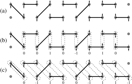
FIG. 8.: (a) One particular spin configuration of Fig. 5. (b) Dashed lines encircling rungs: $S^{z}_{i}=S^{z}_{i,1}+S^{z}_{i,2}$. Notice that after we remove all sites with $S^{z}_{i}=0$, the remaining sites have Néel order. (c) Dashed lines encircling diagonals: $S^{z}_{i}=S^{z}_{i+1,1}+S^{z}_{i,2}$. (Figure adopted from Ref. REFERENCES.)

Now consider the antiferromagnetic ladder with $J_{1}=J$. The ground state is well described by a nearest-neighbor RVB state, for which a typical configuration was shown in Fig. 3. One particular spin configuration is shown in Fig. 9(a). Suppose we look at the $z$ component of the total spin on a rung, as shown in Fig. 9(b); the state has no string order. If, however, we consider the $z$ component of the total spin along plaquette diagonals, as shown in Fig. 9(c), string order is found. It was shown by White[8] that there is a $96.2\%$ probability of finding triplets along plaquette diagonals, and it was verified numerically[8, 9] that these triplets in fact exhibit string order. It was also shown[8, 9] that no string order is found if the total spin along rungs is considered.

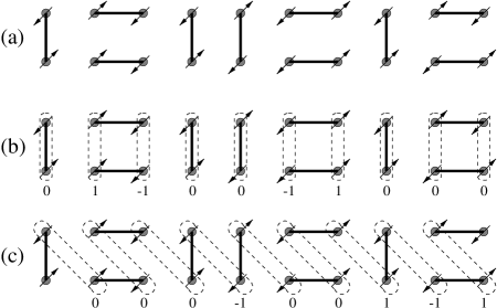
FIG. 9.: (a) One particular spin configuration of Fig. 3. (b) Dashed lines encircling rungs: $S^{z}_{i}=S^{z}_{i,1}+S^{z}_{i,2}$. (c) Dashed lines encircling plaquette diagonals: $S^{z}_{i}=S^{z}_{i+1,1}+S^{z}_{i,2}$. Notice that after we remove all sites with $S^{z}_{i}=0$, the remaining sites have Néel order. (Figure adopted from Ref. REFERENCES.)

As mentioned before, the ladder with ferromagnetic coupling along the rungs is continuously related to the true spin-1 chain. Therefore, it has an AKLT-like ground state and string order due to triplets along the rungs. On the other hand, the ground state of the diagonal ladder with ferromagnetic interchain coupling has an RVB-like ground state, similar to that of the ladder with antiferromagnetic interchain coupling; as discussed above string order is due to triplets along plaquette diagonals.

Finally, consider the zig-zag ladder at the Majumdar-Ghosh point. The exact ground state is given by a product of decoupled singlets, as shown in Fig. 7. One particular spin configuration for Fig. 7(a) is shown in Fig. 10(a). Adding the $z$ components of the spins on the same rung, as shown in Fig. 10(b), it is obvious that we always get zero. However, if we add the spins along plaquette diagonals, as shown in Fig. 10(c), we find string order. Now, however, consider the ground state shown in Fig. 7(b). One particular spin configuration is shown in Fig. 11(a). Then, as shown in Fig. 11(b), if we add the spins along the rungs, we find string order. However, if we add the spins along plaquette diagonals, as shown in Fig. 11(c), we always get zero. This result is not surprising, since it was already shown[12] that the Majumdar-Ghosh ground state has perfect string order. However, it appears that, depending on which of the two degenerate ground states is actually realized, string order can be due to the spins along the rungs or to the spins along plaquette diagonals.

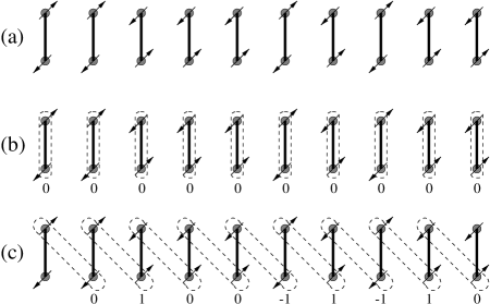
FIG. 10.: (a) One particular spin configuration of Fig. 7(a). (b) Dashed lines encircling rungs: $S^{z}_{i}=S^{z}_{1,i}+S^{z}_{i,2}$. (c) Dashed lines encircling plaquette diagonals: $S^{z}_{i}=S^{z}_{i+1,1}+S^{z}_{i,2}$. Notice that after we remove all sites with $S^{z}_{i}=0$, the remaining sites have Néel order.

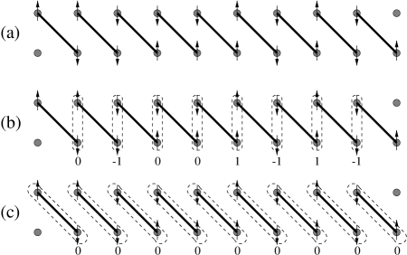
FIG. 11.: (a) One particular spin configuration of Fig. 7(b). (b) Dashed lines encircling rungs: $S^{z}_{i}=S^{z}_{1,i}+S^{z}_{i,2}$. Notice that after we remove all sites with $S^{z}_{i}=0$, the remaining sites have Néel order. (c) Dashed lines encircling plaquette diagonals: $S^{z}_{i}=S^{z}_{i+1,1}+S^{z}_{i,2}$.

  

Motivated by the above examples, similar to Refs. REFERENCES and REFERENCES, we introduce two string order parameters

$${\cal O}^{\alpha}_{\rm odd} = -\lim_{|i-j|\rightarrow\infty}\left\langle(S^{\alpha}_{i,1}+S^{\alpha}_{i,2})\exp\left(i\pi\sum_{l=i+1}^{j-1}(S^{\alpha}_{l,1}+S^{\alpha}_{l,2})\right)(S^{\alpha}_{j,1}+S^{\alpha}_{j,2})\right\rangle\,,$$ (6)

$${\cal O}^{\alpha}_{\rm even} = -\lim_{|i-j|\rightarrow\infty}\left\langle(S^{\alpha}_{i+1,1}+S^{\alpha}_{i,2})\exp\left(i\pi\sum_{l=i+1}^{j-1}(S^{\alpha}_{l+1,1}+S^{\alpha}_{l,2})\right)(S^{\alpha}_{j+1,1}+S^{\alpha}_{j,2})\right\rangle\,.$$ (7)

(The names ${\cal O}_{\rm odd}$ and ${\cal O}_{\rm even}$ will be made clear below.) We saw that when one of the order parameters is finite, the other vanishes. So, the antiferromagnetic ladder has ${\cal O}_{\rm even}\neq 0$; the composite spin model has ${\cal O}_{\rm odd}\neq 0$; the zig-zag ladder at the Majumdar-Ghosh point is special – it can have either ${\cal O}_{\rm even}\neq 0$ or ${\cal O}_{\rm odd}\neq 0$, depending on which of the two degenerate ground states is actually realized. However, it cannot have both finite simultaneously.

Let us now consider the topology of the VB’s in the above examples; an interesting pattern emerges. If we count the number of VB’s crossing an arbitrary vertical line, we find that this number is always even for the ground state configurations of the antiferromagnetic ladder (Fig. 3), while it is always odd for the diagonal ladder at $J_{2}=J$ (Fig. 5). For the zig-zag ladder at the Majumdar-Ghosh point, the number of VB’s crossing an arbitrary vertical line depends on which of the two degenerate ground states we consider: it is even for the state in Fig. 7(a), while it is odd for the state in Fig. 7(b).    

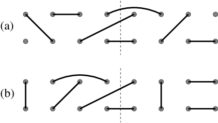
FIG. 12.: Solid lines connecting sites represent VB’s. (a) $Q_{y}=odd$: the number of VB’s crossing a vertical line is odd. (b) $Q_{y}=even$: the number of VB’s crossing a vertical line is even.

These examples are special cases of a more general classification of SR-VB states. It has been shown[21] that for SR-VB configurations on a two-dimensional square lattice, two topological numbers, $Q_{x}=even/odd$ and $Q_{y}=even/odd$, can be defined. They are determined by the parity of the number of SR-VB’s crossing arbitrary horizontal and vertical lines parallel to the $x$- and $y$-axes, respectively. In the case of 2-leg ladders, only $Q_{y}$ is relevant; $Q_{y}$ can be either even or odd, as illustrated more generally in Fig. 12. Hence, there is a topological number which distinguishes between whether the number of SR-VB’s cut by a vertical line is even ($Q_{y}=even$) or odd ($Q_{y}=odd$). For any finite size system, the even and odd sectors are coupled as long as there are VB’s with length comparable to the system size. However, when the system is gapped and thus has a SR-VB ground state, the tunneling amplitude between the two sectors goes to zero exponentially fast as $L\to\infty$, and the ground state is a pure $Q_{y}=even$ or $Q_{y}=odd$ state in the thermodynamic limit. Note that in long-ranged VB ground states of gapless models, the even and odd sectors remain coupled; hence, no such topological distinction is possible.

It is also worth noting that for open boundary conditions $Q_{y}=odd$ ground states have spin-1/2’s localized at the ends of the ladder, while $Q_{y}=even$ states do not. As is obvious from Fig. 12, these end spins occur for topological reasons. Their presence or absence is probably the simplest way to determine $Q_{y}$.

From the above examples, the (topological) parity of the SR-VB ground state and the type of string order seem to be intimately related. It appears that ground states with $Q_{y}=odd$ have ${\cal O}_{\rm odd}$ string order, while ground states with $Q_{y}=even$ have ${\cal O}_{\rm even}$ string order.

Now suppose we smoothly vary the parameters of the Hamiltonian, such that we interpolate between models belonging to different topological classes; a phase transition necessarily occurs. A priori this transition could be either first order or second order, depending on the actual path in parameter space. When the transition is second order, the string order parameters vanish at the transition point and the ground state becomes a long-ranged VB state. In the next section we analyze this problem in the weak coupling limit using bosonization.

IV Weak Coupling Analysis: Bosonization

In the bosonization treatment of the ladder model shown in Fig. 13, we start with two decoupled spin-1/2 chains and treat the interchain couplings perturbatively. Our conventions, as well as the bosonization of spin ladders, are presented in detail in Ref. REFERENCES.

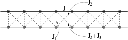
FIG. 13.: Most general ladder model which we will consider, ${\cal H}={\cal H}_{0}+{\cal H}_{1}+{\cal H}_{2}+{\cal H}_{3}$.

The isotropic spin-1/2 Heisenberg chain is known to be critical. The effective Hamiltonian for long wavelength excitations is

$${\cal H}_{s=1/2}=\frac{u}{2}\int dx\left[K\Pi^{2}+\frac{1}{K}(\partial_{x}\Phi)^{2}\right]$$ (8)

where the bosonic phase field, $\Phi$, and its conjugate momentum, $\Pi$, satisfy the commutation relation

$$[\Phi(x),\Pi(y)]=i\delta(x-y)\,.$$ (9)

For an isotropic antiferromagnetic spin chain, $K=1/2$. We will also need the bosonized form of the spin operators. They are[22]

$$S^{+}(x) = {S^{+}_{j}\over\sqrt{a}}=\frac{\exp\left(-i\sqrt{\pi}\Theta\right)}{\sqrt{2\pi a}}\left[e^{-i(\pi x/a)}+\cos(\sqrt{4\pi}\Phi)\right],$$ (10)

$$S^{z}(x) = {S^{z}_{j}\over a}=\frac{1}{\sqrt{\pi}}\partial_{x}\Phi+e^{i(\pi x/a)}\frac{\sin(\sqrt{4\pi}\Phi)}{\pi a}\,,$$ (11)

where the dual field, $\Theta$, is related to $\Pi$ by $\Pi=\partial_{x}\Theta$.

For the ladder, we simply attach a chain index to our fields. Therefore,

$${\cal H}_{0} = \frac{u}{2}\int dx\left[K\Pi_{1}^{2}+\frac{1}{K}(\partial_{x}\Phi_{1})^{2}\right]$$ (13)

$$+\frac{u}{2}\int dx\left[K\Pi_{2}^{2}+\frac{1}{K}(\partial_{x}\Phi_{2})^{2}\right]\,.$$

To bosonize the interchain coupling, we write the spin operators in terms of uniform and staggered components as

$${\bf S}_{i}(x)={\bf J}_{i}(x)+(-1)^{x/a}{\bf n}_{i}(x)\,.$$ (14)

We find

$${\cal H}_{1} \sim J_{1}\int dx\left[{\bf J}_{1}(x)\cdot{\bf J}_{2}(x)+{\bf n}_{1}(x)\cdot{\bf n}_{2}(x)\right],$$ (15)

$${\cal H}_{2} \sim 2J_{2}\int dx\left[{\bf J}_{1}(x)\cdot{\bf J}_{2}(x)-{\bf n}_{1}(x)\cdot{\bf n}_{2}(x)\right],$$ (16)

$${\cal H}_{3} \sim J_{3}\int dx\left[{\bf J}_{1}(x)\cdot{\bf J}_{2}(x)-{\bf n}_{1}(x)\cdot{\bf n}_{2}(x)\right].$$ (17)

Inserting the expressions in Eq. (11) into Eq. (17) gives

$${\cal H}_{i} = \int{dx\over(2\pi a)^{2}}\left[g_{1}^{i}\cos\left(\sqrt{4\pi}(\Phi_{1}+\Phi_{2})\right)\right.$$ (25)

$$\phantom{++}+g_{2}^{i}\cos\left(\sqrt{4\pi}(\Phi_{1}-\Phi_{2})\right)$$

$$\phantom{++}+\left.g_{3}^{i}\cos\left(\sqrt{\pi}(\Theta_{1}-\Theta_{2})\right)\right]$$

$$+\frac{J_{\perp}^{i}}{\pi}\int dx\partial_{x}\Phi_{1}\partial_{x}\Phi_{2}$$

$$+\int\frac{dx}{(2\pi a)^{2}}\left[g_{4}^{i}\cos\left(\sqrt{\pi}(\Theta_{1}-\Theta_{2})\right)\right.$$

$$\phantom{++}\times\cos\left(\sqrt{4\pi}(\Phi_{1}+\Phi_{2})\right)$$

$$\phantom{+}+g_{5}^{i}\cos\left(\sqrt{\pi}(\Theta_{1}-\Theta_{2})\right)$$

$$\left.\phantom{++}\times\cos\left(\sqrt{4\pi}(\Phi_{1}-\Phi_{2})\right)\right]\,.$$

The $g_{1}^{i}$, $g_{2}^{i}$, and $g_{3}^{i}$ terms come from ${\bf n}_{1}(x)\cdot{\bf n}_{2}(x)$, while the $J_{\perp}^{i}$, $g_{4}^{i}$, and $g_{5}^{i}$ terms come from ${\bf J}_{1}(x)\cdot{\bf J}_{2}(x)$.

For ${\cal H}_{1}$:

$$g_{1}^{1}=-2J_{1};\ \ \ g_{2}^{1}=2J_{1};\ \ \ g_{3}^{1}=2\pi J_{1},$$ (26)

$$J_{\perp}^{1}=J_{1};\ \ \ g_{4}^{1}=\pi J_{1};\ \ \ g_{5}^{1}=\pi J_{1}\,.$$ (27)

For ${\cal H}_{2}$:

$$g_{1}^{2}=4J_{2};\ \ \ g_{2}^{2}=-4J_{1};\ \ \ g_{3}^{2}=-4\pi J_{1},$$ (28)

$$J_{\perp}^{2}=2J_{2};\ \ \ g_{4}^{2}=2\pi J_{2};\ \ \ g_{5}^{2}=2\pi J_{2}\,.$$ (29)

For ${\cal H}_{3}$:

$$g_{1}^{3}=2J_{3};\ \ \ g_{2}^{3}=-2J_{3};\ \ \ g_{3}^{3}=-2\pi J_{3},$$ (30)

$$J_{\perp}^{3}=J_{3};\ \ \ g_{4}^{3}=\pi J_{3};\ \ \ g_{5}^{3}=\pi J_{3}\,.$$ (31)

It is useful to define the fields

$$\Phi_{s,a}=\frac{1}{\sqrt{2}}\left(\Phi_{1}\pm\Phi_{2}\right)\,,\ \ \ \Theta_{s,a}=\frac{1}{\sqrt{2}}\left(\Theta_{1}\pm\Theta_{2}\right)\,.$$ (32)

In terms of these fields our Hamiltonian, ${\cal H}={\cal H}_{0}+{\cal H}_{1}+{\cal H}_{2}+{\cal H}_{3}$, is

$${\cal H} = \frac{u_{s}}{2}\int dx\left[K_{s}\Pi_{s}^{2}+\frac{1}{K_{s}}(\partial_{x}\Phi_{s})^{2}\right]$$ (38)

$$+g_{1}\int{dx\over(2\pi a)^{2}}\cos\left(\sqrt{8\pi}\Phi_{s}\right)$$

$$+\frac{u_{a}}{2}\int dx\left[K_{a}\Pi_{a}^{2}+\frac{1}{K_{a}}(\partial_{x}\Phi_{a})^{2}\right]$$

$$+\int{dx\over(2\pi a)^{2}}\left[g_{2}\cos\left(\sqrt{8\pi}\Phi_{a}\right)+g_{3}\cos\left(\sqrt{2\pi}\Theta_{a}\right)\right]$$

$$+g_{4}\int\frac{dx}{(2\pi a)^{2}}\cos\left(\sqrt{2\pi}\Theta_{a}\right)\cos\left(\sqrt{8\pi}\Phi_{s}\right)$$

$$+g_{5}\int\frac{dx}{(2\pi a)^{2}}\cos\left(\sqrt{2\pi}\Theta_{a}\right)\cos\left(\sqrt{8\pi}\Phi_{a}\right)\,,$$

where

$$g_{1} = -2J_{1}+4J_{2}+2J_{3}\ \ \ ,\ \ \ g_{2}=2J_{1}-4J_{2}-2J_{3}\,,$$ (39)

$$g_{3} = 2\pi J_{1}-4\pi J_{2}-2\pi J_{3}\ \ \ ,\ \ \ g_{4}=\pi J_{1}+2\pi J_{2}+\pi J_{3}\,,$$ (42)

$$\hskip 28.90755ptg_{5}=\pi J_{1}+2\pi J_{2}+\pi J_{3}\,,$$

$$\hskip 28.90755ptJ_{\perp}=J_{1}+2J_{2}+J_{3}\,.$$

Also,

$$K_{s}=K\left(1+\frac{KJ_{\perp}}{u\pi}\right)^{-1/2}\,, \ \ \ u_{s}=u\left(1+\frac{KJ_{\perp}}{u\pi}\right)^{1/2}\,,$$ (43)

$$K_{a}=K\left(1-\frac{KJ_{\perp}}{u\pi}\right)^{-1/2}\,, \ \ \ u_{a}=u\left(1-\frac{KJ_{\perp}}{u\pi}\right)^{1/2}\,.$$ (45)

For $J_{\perp}\ll 1$ we have

$$K_{s}\approx K\left(1-\frac{KJ_{\perp}}{2u\pi}\right), \ \ u_{s}\approx u\left(1+\frac{KJ_{\perp}}{2u\pi}\right),$$ (46)

$$K_{a}\approx K\left(1+\frac{KJ_{\perp}}{2u\pi}\right), \ \ u_{a}\approx u\left(1-\frac{KJ_{\perp}}{2u\pi}\right).$$ (47)

We are interested in whether or not the interchain coupling causes a gap in the excitation spectrum. Therefore, we would like to identify the relevant operators; these operators will “pin” their arguments, thus causing gaps to appear. To do this we consider the scaling dimensions of the operators in the interchain coupling.[23, 22] The scaling dimensions of the operators are the following: $\left[\cos\left(\sqrt{8\pi}\Phi_{s}\right)\right]=2K_{s}$; $\left[\cos\left(\sqrt{8\pi}\Phi_{a}\right)\right]=2K_{a}$; $\left[\cos\left(\sqrt{2\pi}\Theta_{a}\right)\right]=1/(2K_{a})$; $\left[\cos\left(\sqrt{2\pi}\Theta_{a}\right)\cos\left(\sqrt{8\pi}\Phi_{s}\right)\right]=2K_{s}+1/(2K_{a})$; $\left[\cos\left(\sqrt{2\pi}\Theta_{a}\right)\cos\left(\sqrt{8\pi}\Phi_{a}\right)\right]=2K_{a}+1/(2K_{a})$. Therefore, $g_{1}$ will grow at large distances for $K_{s}<1$; $g_{2}$ will grow for $K_{a}<1$; $g_{3}$ will grow for $K_{a}>1/4$; $g_{4}$ will grow for $2K_{s}+1/(2K_{a})<2$; $g_{5}$ will grow for $2K_{a}+1/(2K_{a})<2$.

In what follows, we will consider the phases and transitions that occur when we vary $J_{1}$, $J_{2}$, and $J_{3}$. In order to make things more tractable, we will consider two-dimensional slices in the full $J_{1}-J_{2}-J_{3}$ space.

FIG. 14.: Phase diagram for $J_{1}\neq 0$ and $J_{2}\neq 0$ with $J_{3}=0$.

A $J_{1}\neq 0$ and $J_{2}\neq 0$ with $J_{3}=0$

In this case, for $J_{2}=0$ and $J_{1}=J$ we recover the usual antiferromagnetic ladder; for $J_{2}=0$ and $J_{1}\rightarrow-\infty$ we recover a spin-1 chain, where the spins on each rung form an $S=1$. Similarly, for $J_{1}=0$ and $J_{2}=J$ we recover the composite spin representation for a spin-1 chain, and it was previously shown that the composite spin representation has the same low energy physics as the true spin-1 chain.[18]

The phase diagram in the $J_{1}-J_{2}$ plane is shown in Fig. 14. In region $I$ the $g_{1}$ and $g_{3}$ terms are the most relevant. Therefore, $\Phi_{s}$ and $\Theta_{a}$ are pinned with $\langle\Phi_{s}\rangle=(2n+1)\sqrt{\pi/8}$ and $\langle\Theta_{a}\rangle=m\sqrt{2\pi}$. Without loss of generality, we can choose $n=0$ and $m=0$. This gives $\langle\Phi_{s}\rangle=\sqrt{\pi/8}$ and $\langle\Theta_{a}\rangle=0$. In region $II$ the $g_{1}$ and $g_{3}$ terms are again the most relevant. Again, $\Phi_{s}$ and $\Theta_{a}$ are pinned. Now, however, $\langle\Phi_{s}\rangle=n\sqrt{\pi/2}$ and $\langle\Theta_{a}\rangle=(2m+1)\sqrt{\pi/2}$. Choosing $n=0$ and $m=0$, $\langle\Phi_{s}\rangle=0$ and $\langle\Theta_{a}\rangle=\sqrt{\pi/2}$. In region $III$ the $g_{1}$ and $g_{2}$ terms are the most relevant. Therefore, $\Phi_{s}$ and $\Phi_{a}$ are pinned with $\langle\Phi_{s}\rangle=n\sqrt{\pi/2}$ and $\langle\Phi_{a}\rangle=(2m+1)\sqrt{\pi/8}$. Choosing $n=0$ and $m=0$ gives $\langle\Phi_{s}\rangle=0$ and $\langle\Phi_{a}\rangle=\sqrt{\pi/8}$. In region $IV$, similar to region $III$, the $g_{1}$ and $g_{2}$ terms are the most relevant, so $\Phi_{s}$ and $\Phi_{a}$ are pinned. However, in this region $\langle\Phi_{s}\rangle=(2n+1)\sqrt{\pi/8}$ and $\langle\Phi_{a}\rangle=m\sqrt{\pi/2}$. Choosing $n=0$ and $m=0$, $\langle\Phi_{s}\rangle=\sqrt{\pi/8}$ and $\langle\Phi_{a}\rangle=0$. There are also two special lines in the phase diagram. Along the line $J_{2}=J_{1}/2$, the ${\bf n}_{1}\cdot{\bf n}_{2}$ terms vanish and only the ${\bf J}_{1}\cdot{\bf J}_{2}$ terms remain. For $J_{1},J_{2}<0$, the system is gapless; for $J_{1},J_{2}>0$, the $g_{4}$ term is marginally relevant and the system is gapped. However, the ground state is two-fold degenerate (for $J_{1},J_{2}>0$): $\langle\Phi_{s}\rangle=(2n+1)\sqrt{\pi/8}$, $\langle\Theta_{a}\rangle=2m\sqrt{\pi/2}$ or $\langle\Phi_{s}\rangle=2n\sqrt{\pi/8}$, $\langle\Theta_{a}\rangle=(2m+1)\sqrt{\pi/2}$. Choosing $n=0$ and $m=0$, we have $\langle\Phi_{s}\rangle=\sqrt{\pi/8}$, $\langle\Theta_{a}\rangle=0$ or $\langle\Phi_{s}\rangle=0$, $\langle\Theta_{a}\rangle=\sqrt{\pi/2}$. The other special line is $J_{2}=-J_{1}/2$. Along this line the ${\bf J}_{1}\cdot{\bf J}_{2}$ terms vanish and the ${\bf n}_{1}\cdot{\bf n}_{2}$ terms all have the same scaling dimension = 1. Along this line the spectrum is gapped. This line will be discussed in greater detail in Sec. V.

FIG. 15.: Phase diagram for $J_{1}\neq 0$ and $J_{3}\neq 0$ with $J_{2}=0$.

B $J_{1}\neq 0$ and $J_{3}\neq 0$ with $J_{2}=0$

In this case, for $J_{3}=0$ and $J_{1}=J$ we recover the usual antiferromagnetic ladder; for $J_{3}=0$ and $J_{1}\rightarrow-\infty$ we recover a true spin-1 chain. For $J_{1}=J_{3}\neq 0$ we have a zig-zag ladder; in particular, for $J_{1}=J_{3}=2J$ we have the Majumdar-Ghosh point where the ground state is dimerized with two-fold degeneracy.

The phase diagram in the $J_{1}-J_{3}$ plane is shown in Fig. 15. The regions $I$, $II$, $III$, and $IV$ have properties identical to the $J_{1}-J_{2}$ phase diagram discussed above. The line $J_{3}=-J_{1}$ has properties identical to the line $J_{2}=-J_{1}/2$ discussed above, and will be discussed in greater detail in Sec. V. The line $J_{1}=J_{3}$ is special. As pointed out by Nersesyan et al.,[24] we must be careful of the “twist” operators which appear. Along this line, the interchain coupling of the staggered components can be written as

$$H_{{\rm int}}\sim\int dx\ \left[{\bf n}_{1}\partial_{x}{\bf n}_{2}-{\bf n}_{2}\partial_{x}{\bf n}_{1}\right].$$ (48)

Explicitly, the terms are

$$H_{{\rm int}} = g^{\prime}_{1}\int{dx\over(2\pi a)^{2}}\partial_{x}\Phi_{a}\sin\left(\sqrt{8\pi}\Phi_{s}\right)$$ (49)

$$+ g^{\prime}_{2}\int{dx\over(2\pi a)^{2}}\partial_{x}\Phi_{s}\sin\left(\sqrt{8\pi}\Phi_{a}\right)$$ (50)

$$+ g^{\prime}_{3}\int{dx\over(2\pi a)^{2}}\partial_{x}\Theta_{s}\sin\left(\sqrt{2\pi}\Theta_{a}\right)\,,$$ (51)

where $g^{\prime}_{1}$, $g^{\prime}_{2}$, $g^{\prime}_{3}\sim J_{3}$. These terms are subtle because they have non-zero conformal spin. As pointed out in Ref. REFERENCES, a seemingly irrelevant operator with non-zero conformal spin can generate relevant operators. However, since we are only considering the SU(2) symmetric case, the terms generated are less relevant than the ${\bf J}_{1}\cdot{\bf J}_{2}$ terms already present. Therefore, similar to the line $J_{2}=J_{1}/2$, for $J_{3}<0$ the system is gapless; for $J_{3}>0$ the $g_{4}$ term is marginally relevant and the spectrum is gapped, with the ground state being two-fold degenerate.

V Discussion of the Results

As discussed in Sec. III, the two-leg ladder models we have considered can have either ${\cal O}^{\alpha}_{\rm odd}$ or ${\cal O}^{\alpha}_{\rm even}$ string order, but not both simultaneously. In our case, since we are only considering SU(2) symmetric models, ${\cal O}^{x}={\cal O}^{y}={\cal O}^{z}$. Therefore, for simplicity, we focus only on ${\cal O}^{z}$.

To bosonize the string order parameter, we first write it in a more convenient form. Using the identity $\exp\left(i\pi S^{z}\right)=2iS^{z}$, we can write

  

$${\cal O}^{z}_{\rm odd} = \frac{1}{4}\lim_{|i-j|\rightarrow\infty}\left\langle\left(e^{i\pi S^{\alpha}_{i,1}}+e^{i\pi S^{\alpha}_{i,2}}\right)\exp\left(i\pi\sum_{l=i+1}^{j-1}(S^{\alpha}_{l,1}+S^{\alpha}_{l,2})\right)\left(e^{i\pi S^{\alpha}_{j,1}}+e^{i\pi S^{\alpha}_{j,2}}\right)\right\rangle\,,$$ (52)

$${\cal O}^{z}_{\rm even} = \frac{1}{4}\lim_{|i-j|\rightarrow\infty}\left\langle\left(e^{i\pi S^{\alpha}_{i+1,1}}+e^{i\pi S^{\alpha}_{i,2}}\right)\exp\left(i\pi\sum_{l=i+1}^{j-1}(S^{\alpha}_{l+1,1}+S^{\alpha}_{l,2})\right)\left(e^{i\pi S^{\alpha}_{j+1,1}}+e^{i\pi S^{\alpha}_{j,2}}\right)\right\rangle\,.$$ (53)

   

Bosonizing ${\cal O}^{z}_{\rm odd}$ and ${\cal O}^{z}_{\rm even}$ gives

$${\cal O}^{z}_{{\rm even/odd}}=\lim_{|x-y|\rightarrow\infty}\left\langle e^{i\sqrt{2\pi}\Phi_{s}(x)}e^{-i\sqrt{2\pi}\Phi_{s}(y)}\right\rangle\,.$$ (54)

We see that all we need is for $\Phi_{s}$ to get pinned to have string order. The operators for both ${\cal O}^{z}_{\rm odd}$ and ${\cal O}^{z}_{\rm even}$ have the same bosonized form because the nonlocal string operator makes the continuum limit insensitive to physics occurring on the order of a single lattice spacing, such as whether triplets lie predominantly along rungs or along diagonals. Therefore, the bosonized string order parameter tells us that we have string order, but it does not tell us in which topological sector the order exists. Taking into account the physical picture we get from the VB states in Sec. III, we can understand the various regions and transition lines which have been obtained in the phase diagrams by bosonization. The results are summarized in Table I.

TABLE I.: Results for the $J_{1}-J_{2}$ and $J_{1}-J_{3}$ phase diagrams.

	$I$	$II$	$III$	$IV$
$\Phi_{s}$	$\langle\Phi_{s}\rangle=\sqrt{\pi/8}$	$\langle\Phi_{s}\rangle=0$	$\langle\Phi_{s}\rangle=0$	$\langle\Phi_{s}\rangle=\sqrt{\pi/8}$
$\Phi_{a}$, $\Theta_{a}$	$\langle\Theta_{a}\rangle=0$	$\langle\Theta_{a}\rangle=\sqrt{\pi/2}$	$\langle\Phi_{a}\rangle=\sqrt{\pi/8}$	$\langle\Phi_{a}\rangle=0$
Order Parameter	${\cal O}_{\rm odd}$	${\cal O}_{\rm even}$	${\cal O}_{\rm even}$	${\cal O}_{\rm odd}$

$J_{2}=J_{1}/2$:	$J_{2},J_{3}>0$ — first order transition	$J_{2},J_{3}<0$ — second order transition
$(J_{3}=J_{1}$)	$\langle\Phi_{s}\rangle=\sqrt{\pi/8}$ , $\langle\Theta_{a}\rangle=0$ or $\langle\Phi_{s}\rangle=0$ , $\langle\Theta_{a}\rangle=\sqrt{\pi/2}$	$\Phi_{s}$ and $\Phi_{a}$ critical
$J_{2}=-J_{1}/2$:	level crossing in the excited states
$(J_{3}=-J_{1})$

A $J_{1}\neq 0$ and $J_{2}\neq 0$ with $J_{3}=0$

The line $J_{1}=0$ with $J_{2}>0$ is continuously related to the composite spin model; the composite spin model has ${\cal O}_{\rm odd}$ string order. Therefore, it appears that region $I$ is continuously related to this model, and hence has ${\cal O}_{\rm odd}$ string order. The line $J_{2}=0$ with $J_{1}>0$ is continuously related to the usual antiferromagnetic ladder; the antiferromagnetic ladder has ${\cal O}_{\rm even}$ string order. Therefore, it appears that region $II$ is continuously related to this model, and hence has ${\cal O}_{\rm even}$ string order. Along the line $J_{1}=0$ with $J_{2}<0$, we have ferromagnetic interchain coupling along plaquette diagonals. For $|J_{2}|\approx J_{1}$ the ground state is similar to the RVB state of the ladder with antiferromagnetic interchain coupling. Hence, this model has ${\cal O}_{\rm even}$ string order. It appears that region $III$ is continuously related to this model, and hence has ${\cal O}_{\rm even}$ string order. Finally, the line $J_{2}=0$ with $J_{1}<0$ is continuously related to the spin-1 chain in which the spins on a rung form an effective $S=1$. Since the ground state of the spin-1 chain is described by the AKLT state, this model has ${\cal O}_{\rm odd}$ string order. Therefore, it appears that region $IV$ is continuously related to this model, and hence has ${\cal O}_{\rm odd}$ string order. We see that a transition between ${\cal O}_{\rm odd}$ and ${\cal O}_{\rm even}$ string order occurs along the line $J_{2}=J_{1}/2$. For $J_{2}<0$ the transition is second order; for $J_{2}>0$, there is a marginally relevant operator which drives the transition first order. The line $J_{2}=-J_{1}/2$ is interesting, so we discuss it in detail.

Along the line $J_{2}=-J_{1}/2$ there is a change in the properties of the system: above the line, $\Theta_{a}$ is pinned; below the line, $\Phi_{a}$ is pinned. However, we believe this is a level crossing in the excited states; the properties of the ground state remain the same. Hence, the system does not undergo a phase transition when we cross this line. To show this, it is useful to express ${\cal H}_{a}$ in terms of Majorana fermions. We begin on the line $J_{2}=-J_{1}/2$; along this line, the ${\bf J}_{1}\cdot{\bf J}_{2}$ terms vanish and the ${\bf n}_{1}\cdot{\bf n}_{2}$ terms all have the same scaling dimension. Rescaling our fields,

$$\Pi_{a}\rightarrow\frac{1}{\sqrt{K_{a}}}\Pi_{a}\ \ \ ,\ \ \ \Phi_{a}\rightarrow\sqrt{K_{a}}\Phi_{a}\,,$$ (55)

${\cal H}_{a}$ has the form

$$\hskip 32.52127pt{\cal H}_{a}=\frac{u_{a}}{2}\int dx\left[\Pi_{a}^{2}+(\partial_{x}\Phi_{a})^{2}\right]$$ (56)

$$+\int{dx\over(2\pi a)^{2}}\left[g_{2}\cos\left(\sqrt{4\pi}\Phi_{a}\right)+g_{3}\cos\left(\sqrt{4\pi}\Theta_{a}\right)\right]\,.$$ (57)

Using that[23]

$$\frac{u}{2}\int dx\left[\Pi^{2}+(\partial_{x}\Phi)^{2}\right]$$ (58)

$$\hskip 28.90755pt=-iu\int dx\left[\psi_{R}^{\dagger}\partial_{x}\psi_{R}-\psi_{L}^{\dagger}\partial_{x}\psi_{L}\right]\,,$$ (59)

$$\frac{1}{\pi a}\cos(\sqrt{4\pi}\Phi)=i\left(\psi_{R}^{\dagger}\psi_{L}-\psi_{L}^{\dagger}\psi_{R}\right)\,,$$ (60)

$$\frac{1}{\pi a}\cos(\sqrt{4\pi}\Theta)=i\left(\psi_{R}^{\dagger}\psi_{L}^{\dagger}-\psi_{L}^{\dagger}\psi_{R}^{\dagger}\right)\,,$$ (61)

${\cal H}_{a}$ can be written as

$${\cal H}_{a} = -iu_{a}\int dx\left(\psi_{a,R}^{\dagger}\partial_{x}\psi_{a,R}-\psi_{a,L}^{\dagger}\partial_{x}\psi_{a,L}\right)$$ (62)

$$+ \frac{i}{2}\int\frac{dx}{2\pi a}\left[g_{2}\left(\psi_{a,R}^{\dagger}\psi_{a,L}-\psi_{a,L}^{\dagger}\psi_{a,R}\right)\right.$$ (64)

$$\hskip 14.45377pt\left.+g_{3}\left(\psi_{a,R}^{\dagger}\psi_{a,L}^{\dagger}-\psi_{a,L}^{\dagger}\psi_{a,R}^{\dagger}\right)\right].$$

Now introduce two independent Majorana fermions, $\xi$ and $\eta$, defined by

$$\psi_{a,R}=\frac{1}{\sqrt{2}}(\xi_{R}+i\eta_{R})\ \ \ ,\ \ \ \psi_{a,L}=\frac{1}{\sqrt{2}}(\xi_{L}+i\eta_{L})\,.$$ (65)

Finally, ${\cal H}_{a}$ can be written as

$${\cal H}_{a} = \frac{-iv_{a}}{2}\int dx\left[(\xi_{R}\partial_{x}\xi_{R}-\xi_{L}\partial_{x}\xi_{L})\right.$$ (67)

$$\hskip 61.42993pt+\left.(\eta_{R}\partial_{x}\eta_{R}-\eta_{L}\partial_{x}\eta_{L})\right]$$

$$+ \frac{i}{2}\int\frac{dx}{2\pi a}\left[(g_{2}-g_{3})\xi_{R}\xi_{L}+(g_{2}+g_{3})\eta_{R}\eta_{L}\right].$$ (68)

This is the Hamiltonian for two massive Majorana fermions. As is well known, massive Majorana fermions describe the long distance properties of the Ising model away from criticality.

For $J_{2}\approx-J_{1}/2$ (i.e. $J_{2}=-J_{1}/2+\delta$, $|\delta|\ll 1$), the ${\bf J}_{1}\cdot{\bf J}_{2}$ terms do not vanish. However, very close to the line $J_{2}=-J_{1}/2$, we can still write ${\cal H}_{a}$ in terms of Majorana fermions. The ${\bf J}_{1}\cdot{\bf J}_{2}$ terms can be written as four-fermion interactions which just renormalize the velocity and fermion masses [25]. The key thing to notice is that when we cross the line $J_{2}=-J_{1}/2$, the values of the fermion masses change, but their signs do not change. It is well known that the (Majorana) fermion mass changing sign corresponds to the order-disorder transition of the Ising model. Since there is no change in sign when we cross the line $J_{2}=-J_{1}/2$, the structure of the ground state does not appear to change. Therefore, we interpret the change from $\Theta_{a}$ being pinned to $\Phi_{a}$ being pinned as a level crossing in the excited states. Hence, the system does not appear to undergo a phase transition when crossing this line.

B $J_{1}\neq 0$ and $J_{3}\neq 0$ with $J_{2}=0$

The line $J_{1}>0$ with $J_{3}=0$ is continuously related to the usual antiferromagnetic ladder; the antiferromagnetic ladder has ${\cal O}_{\rm even}$ string order. Therefore, it appears that region $II$ is continuously related to this model, and hence has ${\cal O}_{\rm even}$ string order. The line $J_{1}<0$ with $J_{3}=0$ is continuously related to the spin-1 chain in which the spins on a rung form an effective $S=1$. Since the ground state of the spin-1 chain is described by the AKLT state, this model has ${\cal O}_{\rm odd}$ string order. Therefore it appears that region $IV$ is continuously related to this model, and hence has ${\cal O}_{\rm odd}$ string order. Along the line $J_{1}=0$, the coupling along the rungs is zero and only the diagonal interchain coupling, $J_{3}$, is nonzero. This is similar to the case when only $J_{1}\neq 0$, except with chain-1 shifted to the right by one lattice spacing. Therefore, $J_{3}>0$ is similar to the usual antiferromagnetic ladder and $J_{3}<0$ is similar to the spin-1 chain, except with chain-1 shifted to the right by one lattice spacing. Hence, $J_{3}>0$ has ${\cal O}_{\rm odd}$ string order, and $J_{3}<0$ has ${\cal O}_{\rm even}$ string order. It appears that region $I$ is continuously related to the line $J_{3}>0$ and that region $III$ is continuously related to the line $J_{3}<0$. Therefore, region $I$ has ${\cal O}_{\rm odd}$ string order and region $III$ has ${\cal O}_{\rm even}$ string order. A phase transition occurs along the line $J_{3}=J_{1}$. For $J_{3}<0$ the transition is second order, while for $J_{3}>0$ a marginally relevant operator drives the transition first order. Similar to the line $J_{2}=-J_{1}/2$, the system changes character when crossing the line $J_{3}=-J_{1}$. Above the line, $\Theta_{a}$ is pinned; below the line $\Phi_{a}$, is pinned. Similarly, we believe that there is no phase transition as we cross this line; it is a level crossing in the excited states.

It is interesting to note that in our model, the zig-zag ladder (i.e. the line $J_{3}=J_{1}$) is actually a transition line. For $J_{3}>0$ the line is a first order transition line, while for $J_{3}<0$ the transition is second order. Therefore, the Majumdar-Ghosh point actually lies on a first order transition line.

VI Concluding Remarks

In this paper we studied the gapped phases in two-leg spin ladders. The ground states of these ladders are well described by SR-VB states. There are two topologically distinct classes characterized by whether the number of VB’s cut by a vertical line is even ($Q_{y}=even$) or odd ($Q_{y}=odd$). Note that this classification of $Q_{y}=even$ and $Q_{y}=odd$ can be used for even-leg ladders but not for odd-leg ladders. For odd-leg ladders, one gets an even-odd alternation, as shown schematically in Fig. 16. This even-odd alternation implies a two-fold degenerate ground state, consistent with the Lieb-Schultz-Mattis theorem.[21]

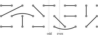
FIG. 16.: A VB configuration which could occur for a three-leg ladder, provided the couplings are chosen so that the ground state is described by a SR-VB state. Notice that the number of bonds crossing a vertical line alternates.

Associated with $Q_{y}=even$ and $Q_{y}=odd$, we considered the “even” and “odd” string order parameters of Eq. 7 for the ladder model shown in Fig. 13. Using known results for particular values of the coupling constants along with bosonization, we obtained the phase diagrams in the $J_{1}-J_{2}$ and $J_{1}-J_{3}$ planes, shown in Figs. 14 and 15, respectively. While these results cover only parts of the $J_{1}-J_{2}-J_{3}$ parameter space, we believe that the association of the string order parameters ${\cal O}^{\alpha}_{\rm even}$ and ${\cal O}^{\alpha}_{\rm odd}$ with $Q_{y}=even$ and $Q_{y}=odd$ is appropriate for this model in general.

We should emphasize that this classification of $Q_{y}=even$ and $Q_{y}=odd$ relies on the possibility of writing the singlet ground state of the ladder as a superposition of VB configurations. This may break down in anisotropic models, and so by introducing anisotropic couplings the two topological sectors may be coupled.

Another interesting problem is related to the spin-1 chain with bilinear and biquadratic exchange interactions[26] and spin ladders with 4-spin plaquette couplings,[19, 27] both having a non-Haldane-like dimerized phase. Although $Q_{y}$ is still a good topological number for the dimerized ground state, it is not clear if string order is simply due to the short-ranged nature of the VB’s and survives the transition from the Haldane phase to the dimerized phase.

It is clear from this analysis that the apparently featureless spin liquid phase of spin-gapped two-leg ladders actually has a rich underlying topological structure. It remains to be seen what role these ideas may play in the doped systems. More precisely, does this topological structure survive when the system is doped, and is pairing ultimately related to the topological structure?

REFERENCES

- [1] H. Bethe, Z. Phys. 71, 205 (1931).
- [2] F. D. M. Haldane, Phys. Rev. Lett. 50, 1153 (1983); Phys. Lett. 93A, 464 (1983).
- [3] G. Sierra, in Strongly Correlated Magnetic and Superconducting Systems, Lecture Notes in Physics, vol. 478, edited by G. Sierra and M. A. Martin-Delgado, Springer-Verlag (1997).
- [4] I. Affleck, T. Kennedy, E. H. Lieb, and H. Tasaki, Phys. Rev. Lett. 59, 799 (1987); Commun. Math. Phys. 115, 477 (1988).
- [5] M. P. M. den Nijs and K. Rommelse, Phys. Rev. B 40, 4709 (1989).
- [6] For reviews see E. Dagotto and T. M. Rice, Science 271, 618 (1996); T. M. Rice, Z. Phys. B 103, 165 (1997); E. Dagotto, cond-mat/9908250.
- [7] E. Dagotto, J. Riera, and D. J. Scalapino, Phys. Rev. B 45, 5744 (1992).
- [8] S. R. White, Phys. Rev. B 53, 52, (1996).
- [9] Y. Nishiyama, N. Hatano, and M. Suzuki, J. Phys. Soc. Jpn. 64, 1967 (1995).
- [10] See S. Watanabe and H. Yokoyama, J. Phys. Soc. Jpn. 68, 2073 (1999), and references therein.
- [11] C. K. Majumdar and D. K. Ghosh, J. Math. Phys. 10, 1388, (1969).
- [12] K. Hida, Phys. Rev. B 45, 2207 (1992).
- [13] A. K. Kolezhuk and H.-J. Mikeska, Phys. Rev. B 56, R11 380 (1997).
- [14] T. Barnes and J. Riera, Phys. Rev. B 50, 6817 (1994).
- [15] S. R. White, R. M. Noack, and D. J. Scalapino, Phys. Rev. Lett. 73, 886 (1994).
- [16] H. Watanabe, K. Nomura, and S. Takada, J. Phys. Soc. Jpn. 62, 2845 (1993); H. Watanabe, Phys. Rev. B 50, 13 442 (1994).
- [17] T. Barnes, E. Dagotto, J. Riera, and E. S. Swanson, Phys. Rev. B 47, 3196 (1993).
- [18] J. Sólyom and J. Timonen, Phys. Rev. B 34, 487 (1986); 38, 6832 (1988); 39, 7003 (1989).
- [19] Ö. Legeza, G. Fáth, and J. Sólyom, Phys. Rev. B 55 291 (1997).
- [20] S. R. White and I. Affleck, Phys. Rev. B 54, 9862 (1996).
- [21] N. E. Bonesteel, Phys. Rev. B 40, 8954 (1989).
- [22] E. H. Kim and J. Sólyom, to appear in Phys. Rev. B 60 (1999); cond-mat/9903241.
- [23] A. M. Tsvelik, Quantum Field Theory in Condensed Matter Physics, Cambridge University Press (1995).
- [24] A. A. Nersesyan, A. O. Gogolin, and F. H. L. Essler, Phys. Rev. Lett. 81, 910 (1998).
- [25] D. G. Shelton, A. A. Nersesyan, A. M. Tsvelik, Phys. Rev. B 53, 8521 (1996).
- [26] G. Fáth and J. Sólyom, Phys. Rev. B 51 3620 (1995).
- [27] A. A. Nersesyan and A. M. Tsvelik, Phys. Rev. Lett. 78, 3939 (1997).