[

Stable and unstable vortices in multicomponent Bose-Einstein condensates

Abstract

We study the stability and dynamics of vortices in two-species condensates as prepared in the recent JILA experiment ( M. R. Andrews et al., Phys. Rev. Lett. 83 (1999) 2498). We find that of the two available configurations, in which one specie has vorticity $m=1$ and the other one has $m=0$, only one is linearly stable, which agrees with the experimental results. However, it is found that in the unstable case the vortex is not destroyed by the instability, but may be transfered from one specie to the other or display complex spatiotemporal dynamics.

]

Vortices appear in many different physical contexts ranging from classical phenomena such as fluid mechanics [1] and nonlinear Optics [2] to purely quantum phenomena such as superconductivity and superfluidity [3]. In the last two years more than 100 papers concerning vortices have been published in Physical Review Letters, which is a naive way to appreciate the importance of this subject in Physics.

A vortex is the simplest topological defect one can construct: in a closed path around a vortex, the phase of the field undergoes a $2\pi$ winding and stabilizes a zero value of the field placed in the vortex core. The vortex is stable because of topological constraints; removing the phase singularity implies an effect on the boundaries of the system which cannot be achieved using local perturbations.

Vortices are central to our understanding of superfluidity and quantized flow. This is why after the experimental realization of Bose-Einstein condensates (BEC) with ultracold atomic gases [4] the question of whether atomic BEC’s are superfluids has triggered the analysis of vortices. The main goals up to now have been to propose a robust mechanism to generate [5, 6] and detect vortices [7]. But another important research area is the analysis of vortex stability [8, 9, 10], to which this works contributes.

Although most of the theoretical effort concerning vortices has been focused on single component condensates, the first experimental production of vortices in a BEC was attained using a two-species ⁸⁷Rb condensate [11]. In this experiment the condensed cloud is made up of atoms in two different hyperfine levels, denoted by $|1\rangle$ and $|2\rangle$. Since the scattering lengths are different both states are not equivalent. As a consequence, while each specie can host a vortex, in Ref. [11] it was shown that a single vortex is stable only when it is placed in the component with the largest scattering length, $|1\rangle$. The other possibility, which has the vortex in $|2\rangle$, leads to some kind of instability.

Our intention is to prove in this paper that the instability is purely dynamical and can be explained with a mean field model which does not include any type or dissipation. We will achieve this goal in three major steps. First, we propose a model based on coupled Gross-Pitaevskii equations and solve the stationary equations in two and three-dimensional setups. We obtain the lowest energy stationary states that can be qualitatively identified with the ground state and the two realizations of Ref. [11]. Next we study the stability of each state under small perturbations using linear perturbation theory. Our main result is that only the experimentally stable configuration is also linearly stable. Finally, using numerical simulations, we study more realistic conditions in which the condensate suffers moderate to strong perturbations. We show that there is a good agreement with experiment and also that the dynamics is very rich and depends on the dimensionality of the system and the intensity of the perturbations.

The model.- In this work we will use the zero temperature approximation, in which collisions between the condensed and non condensed atomic clouds are neglected. In the two species case this leads to a pair of coupled Gross-Pitaevskii equations (GPE)

$$i\hbar\frac{\partial}{\partial t}\psi_{1} = \left[-\frac{\hbar^{2}\nabla^{2}}{2m}+V_{1}+\tilde{u}_{11}|\psi_{1}|^{2}+\tilde{u}_{12}|\psi_{2}|^{2}\right]\psi_{1},$$ (2)

$$i\hbar\frac{\partial}{\partial t}\psi_{2} = \left[-\frac{\hbar^{2}\nabla^{2}}{2m}+V_{2}+\tilde{u}_{21}|\psi_{1}|^{2}+\tilde{u}_{22}|\psi_{2}|^{2}\right]\psi_{2}.$$ (3)

where $\tilde{u}_{ij}=\frac{4\pi\hbar^{2}}{m}a_{ij}$, and $a_{ij}$ are the corresponding scattering length. To simplify the formalism and in analogy with experiments we assume that both potentials are spherically symmetric, i. e. $V_{1}(\vec{r})=V_{2}(\vec{r})=\frac{1}{2}m\omega^{2}(r^{2}+z^{2}).$

Following the experiments, we will present results for equal number of particle on each specie, $N_{1}=N_{2}=N$, which translates to

$$\int|\psi_{1}(\vec{r})|^{2}d\vec{r}=\int|\psi_{2}(\vec{r})|^{2}d\vec{r}\equiv 1.$$ (4)

after a proper rescaling of $\psi_{1}$ and $\psi_{2}$ by $N$. To simplify the analysis we change to a new set of units based on the trap characteristic length, $a_{0}=\sqrt{\hbar/m\omega}$, and period, $\tau=1/\omega$. In this set of units the nonlinear coefficients are $u_{ij}=4\pi a_{ij}\sqrt{N_{i}N_{j}}/a_{0}$. For the JILA experiment, in which $\omega=2\pi\times 7.8\pm 0.1Hz$, we have that $\tau\simeq 20.4\ \hbox{ms}$ is the new unit of time.

The whole study, including the linear stability analysis and the numerical simulations, was performed in two- and three-dimensional systems. We have studied the system up to values of $u_{ij}\leq 5000$, which are of the order of magnitude of the experiments. Nevertheless, the linear stability analysis and the simulations change little for the strongest interactions and we expect our results to be still valid for a larger number of particles ($N\gg 10^{6}$). Regarding the intensity of the nonlinearity, we have used the scattering lengths of $\,{}^{87}$Rb which appear in Ref. [12]. These values give us a precise line in the parameter space

$$U=g\left(\begin{array}[]{cc}1.00&0.97\\ 0.97&0.94\end{array}\right).$$ (5)

It is remarkable that because of the relation $u_{11}>u_{12}>u_{22}$ the experiment is performed in a regime in which the first component chases the second one, which rejects mixing with the chaser. This means that a “desired” configuration has the first component spread over the largest part of the space. As we will see, this has important consequences for the dynamic of the states.

Search of solutions.- We are interested in stationary configurations in which each component has a well defined value of the angular momentum. Such states have the time and angular dependence factored out

$$\psi_{i}(r,z,\theta)=e^{-i\mu_{i}t}e^{im_{i}\theta}\phi_{i}(r,z).$$ (6)

These functions satisfy a nonlinear set of coupled PDE

$$\mu_{t}\psi_{i}=-\frac{1}{2}\nabla^{2}\psi_{i}+\frac{1}{2}\left(r^{2}+z^{2}\right)\psi_{i}+\sum_{j}u_{ij}|\psi_{j}|^{2}\psi_{i},$$ (7)

with $i=1,2$. Our focus will be on three particular configurations, which are the lowest energy states with vorticities $(m_{1},m_{2})=(0,0),(1,0),(0,1)$. They correspond to the ground state of the double condensate, and to the single vortex states for the $|1\rangle$ and $|2\rangle$ species, respectively.

To find the radial and longitudinal dependences of the wave functions, $\phi_{i}(r,z)$, we expand them approximately on a finite subset of the harmonic oscillator basis, $\phi_{i}(r,z)\simeq\sum_{n=0}^{n=N}c_{n}P_{n}^{(m_{i})}(r,z)e^{-r^{2}/2}e^{-z^{2}/2}$ and then search the ground states for each of the $(m_{1},m_{2})$ pairs of vorticities. The details of the method applied to single vortex systems can be found in Ref. [10]. As a result one obtains the desired eigenfunctions, chemical potential and energies [Fig. 1(a)] of each $(m1,m2)$ ground state.

Linear stability analysis.- Let us study the behavior of the stationary states under infinitesimal perturbations (e.g. in the initial data, small amounts of noise, etc.). To do so, we define the excitations as

$$\psi_{i}(r,z,\theta) = e^{-i\mu_{i}t+im_{i}\theta}\left(\phi_{i}(r,z)+e^{-i\lambda t+in\theta}\alpha_{i}(r,z)\right),$$ (9)

$$\bar{\psi}_{i}(r,z,\theta) = e^{i\mu_{i}t-im_{i}\theta}\left(\bar{\phi}_{i}(r,z)+e^{-i\lambda t-in\theta}\beta_{i}(r,z)\right).$$ (10)

Then we introduce Eqs. (Stable and unstable vortices in multicomponent Bose-Einstein condensates) into Eq. (Stable and unstable vortices in multicomponent Bose-Einstein condensates) and keep the ${\cal O}(\alpha)$ and ${\cal O}(\beta)$ terms. In the end we reach an equation for the perturbations $\vec{W}=[\alpha,\alpha^{*},\beta,\beta^{*}]$ which is of the type $iJ\partial_{t}\vec{W}=H\vec{W}$. Here $H$ is an hermitian operator and $iJ$ is an anti-hermitian operator. We will search a Jordan basis such that $\lambda\vec{W}=-iJH\vec{W}.$ The lack of such a Jordan form leads to polynomial instabilities, while the presence of non-real eigenvalues is a signal of the exponentially growing instabilities. All other modes give us the frequencies of the linear response of the system to small perturbations.

This analysis is formally equivalent to the Bogoliubov stability analysis of the states under consideration. However, as it was shown in [10], our perturbation is of order ${\cal O}(\alpha^{2},\beta^{2})$ in the energy and thus the exponentially unstable modes lay along directions of constant energy and thus a Bogoliubov expansion of the Hamiltonian cannot account for the instability, which can only be reached by working directly on the GPE. It is thus important to confirm our linear stability results with numerical simulations of the whole system.

Linear stability results.- When we perform the diagonalization on $(m_{1},m_{2})=(0,0)$ we obtain that all of the eigenvalues are positive numbers, which implies that $(0,0)$ is at least a local minimum of our energy functional –furthermore, it is the ground state of the system and thus globally stable.

Next we studied the $(1,0)$ family [Fig. 1(c)] and find that there is a negative eigenvalue among an infinite number of positive ones, which means that there is a single path in the configuration space along which the energy decreases. That direction belongs to a $m=0$ perturbation which takes the vortex out of the condensate [9]. Nevertheless, as in this case there exist no complex eigenvalues, we conclude that the lifetime of the configuration is only limited by the presence and amount of the losses. This is confirmed when take a $(1,0)$ configuration, perturb it and study its real time evolution [Fig. 1(d)], and it is indeed consistent with the experiments of Ref. [11].

We must remark that the existence of a negative eigenvalue in the spectrum around the $(1,0)$ vortex contradicts the belief that the second component could act as a pinning potential. Indeed, based on further study we can state that a $(1,0)$ vortex remains energetically unstable even for different proportions of each specie, from $N_{1}\simeq 0$ to $N_{2}\simeq 0$ [13].

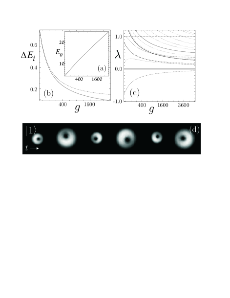
FIG. 1.: (a) Energy of the ground state, $(0,0)$, (b) energy of the $(1,0)$ (solid line) and $(0,1)$ (dashed line) configurations relative to the ground state and (c) frequencies of the linear modes around the $(1,0)$ stable state, with respect to the nonlinearity, given by $g$ [Eq. (5)]. (d) Upper view of component $|1\rangle$ with a vortex after a strong perturbation of the cloud (see above) for $g=1500$. Pictures are equispaced by 10 time units and each one is $18\times 18$ spatial units large.

Finally we focus on the $(0,1)$ family [Fig. 2(a)]. Here we find an infinite number of modes with positive energy, plus a pair of them with negative frequency and complex eigenvalues, $\lambda_{u}$. Qualitatively, the shape and frequencies of the unstable modes are similar to those of the energy decreasing modes of the $(1,0)$ –that is, they are perturbations which push the vortex out of both clouds. The difference is that due to the imaginary part of those eigenvalues, which is Im$(\lambda_{u})={\cal O}(0.04)$ [Fig. 2(b)], vortices with unit charge in $|2\rangle$ are unstable under a generic perturbation of the initial data. This is consistent with the JILA experiments, where the a vortex hosted inside a $|2\rangle$ specie was found to be unstable.

Although, as we mentioned above, the previous result does not depend drastically on $N_{1}$ being equal to $N_{2}$, we have also found that for $N_{2}\gg N_{1}$ the vortex in $|2\rangle$ becomes practically stable [13] –that is, the lifetime is too long to be observed in numerical simulations. This is consistent with the limit of a single-specie condensate where the unit-charge vortex is found to be stable [10] for any scattering length.

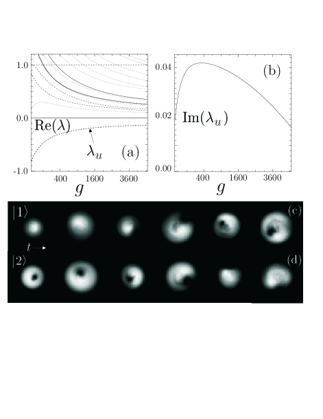
FIG. 2.: (a) Linear response frequencies around the $(0,1)$ unstable state and (b) imaginary part of the unstable mode arising from the linear stability analysis, both with respect to the nonlinearity $g$ [Eq. (5)] (c-d) Upper view of an unstable vortex after a finite perturbation for $g=1500$. Shown are species $|1\rangle$ (c) and $|2\rangle$ (d). Pictures are equispaced by 10 time units and each one is $18\times 18$ units large.

Does the vortex break?.- The linear stability analysis cannot be used to draw conclusions about the behavior of the vortex far from the limit of infinitesimal perturbations. To get further insight on the dynamics we have performed a set of numerical simulations in which we reproduce different realistic perturbations of each state. These perturbations vary from small displacements of the vortex core which should agree in detail with the linear stability results, to strong perturbations of the initial data. In particular, we have systematically used the procedure of creating a stationary state and then reducing the size of the trap, thus transfering the system to a non stationary state [16]. The numerical simulations have been done using a symmetrized split-step Fourier pseudospectral method on grids of sizes ranging from $32\times 32\times 32$ to $64\times 64\times 64$ for the three-dimensional setups, and $64\times 64$ to $256\times 256$ for the two-dimensional model. All results were tested on different grid sizes and changing time steps to ensure their validity.

From our numerical simulations we extract several conclusions. First, the linearly stable state, $(1,0)$, is also a robust one and survives to an ample range of perturbations, suffering at most a precession of the vortex core plus changes of the shapes of both components [Fig. 1(d)]. This behavior is equally reproduced in two- and three-dimensional simulations.

Next we have the unstable states, $(0,1)$ subject to weak perturbations in either two- or three-dimensional models. In that case the unstable configuration develops a simple recurrent dynamics, which is well represented by Figs. 2(d-e). There we see a first stage where the first component [Fig. 2(d)] and the vortex [Fig. 2(e)] oscillate synchronously (the hole in $|2\rangle$ pins the peak of $|1\rangle$). These oscillations grow in amplitude until the linked system spirals out and forms a ying-yang which rotates clockwise, one specie chasing the other. Finally the first component develops a tail and later a hole which traps the second component. That hole is a vortex, which somehow has been transfered from $|2\rangle$ to $|1\rangle$. Though it is not completely periodic, this mechanism does exhibit some recurrence and the vortex returns to $|2\rangle$.

The preceding behavior persists even for strong perturbations in a two-dimensional condensate. However, when one considers a three dimensional condensate and applies large perturbations on the initial data such as the one described above, it is possible to find a richer dynamics which include the establishment of spatiotemporal chaos. As an example, Fig. 3 shows a regime in which more than one vortex are introduced into the first component for long times. Intuitively, this turbulent behavior has two causes. First, due to energetic considerations there is a bigger overlap of both species than in the two dimensional model, as is apparent from the pictures. And second and most important, in the a three dimensional environment the first component is more reluctant to be dragged by the weak vortex-line from the second component. Thus, as the second component spirals around, it is able to shake the first fluid and produce pairs of vortices, much like what happens in laser-stirred condensates [6].

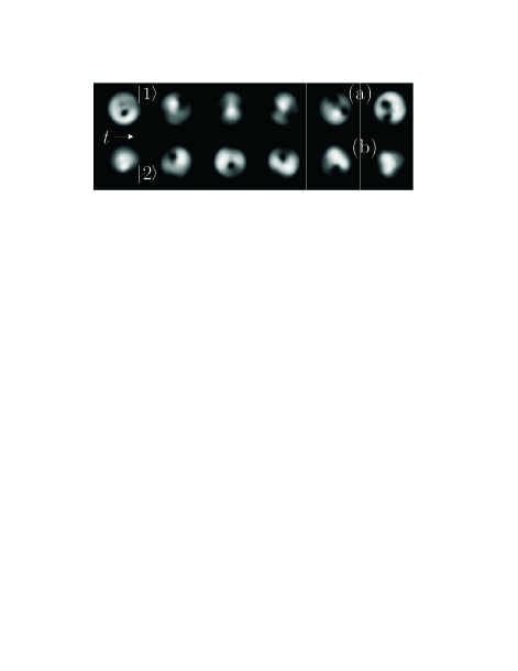
FIG. 3.: Evolution of an unstable $(0,1)$ configuration subject to a finite perturbation after a 50 units run for $g=1500$. Spatiotemporal chaos with several vortices develops for long enough times. Shown are upper views equispaced by 10 time units, each one $18\times 18$ spatial units large.

Either phenomena, the transfer of the vortex and the chaotic evolution do not not contradict any topological rule or conservation law. In fact the angular momentum of each component is no longer a conserved quantity, and the topological charge of each specie needs not survive through the evolution. Instead, what is conserved is the total angular momentum

$$L_{z}=i\hbar\int{\bar{\psi}}_{1}\partial_{\theta}\psi_{1}+i\hbar\int{\bar{\psi}}_{2}\partial_{\theta}\psi_{2}=L_{z}^{(1)}+L_{z}^{(2)}.$$ (11)

In Fig. 4 we plot the evolution of the total angular momentum and that of each component $L_{z}^{(j)}$ for a recurrent situation and for the case of a spatiotemporally chaotic state [Fig. 3]. It can be seen that there is a complex interchange of angular momentum between both components. The intermediate states are topologically nontrivial ones since the phase singularity is being transfered from one component to the other. A more detailed analysis of this process will be presented elsewhere [13].

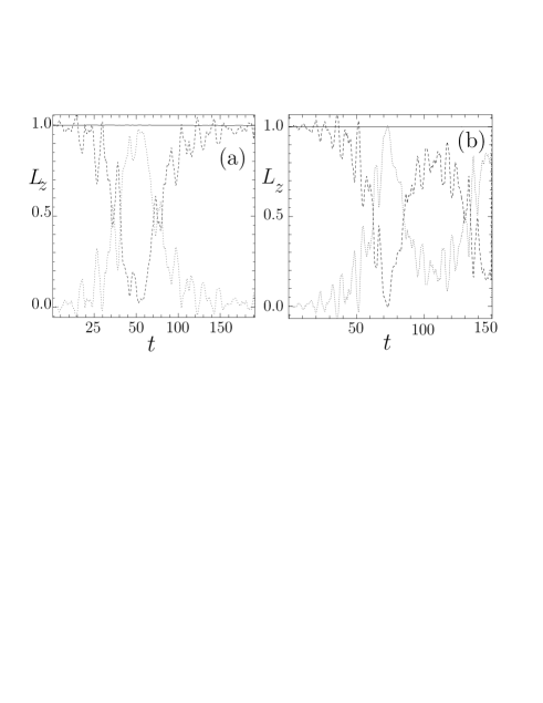
FIG. 4.: Evolution of total angular momenta $L_{z}$ (solid line, well conserved by our numerical scheme), and partial angular momenta $L_{z}^{(1)}$ (dotted line) and $L_{z}^{(2)}$ (dashed line), with respect to time in adimensional units. Plot (a) belongs to a situation with a simple, recurrent transfer of the vortex, while (b) corresponds to a chaotic spatiotemporal dynamics [Fig. 3].

Conclusions and discussion.- We have analyzed the stability of vortices in multi-component atomic Bose-Einstein condensates, using both two-dimensional and three-dimensional sets of coupled Gross-Pitaevskii equations. We prove that a vortex in a $|1\rangle$ state is a dynamically stable object even though it is not a global minimum of the energy. In contrast, we demonstrate that a vortex in the $|2\rangle$ specie is dynamically and energetically unstable and tends to spiral out of the condensate. Besides, since our model does not involve dissipative effects or asymmetries, one cannot get rid of the vortex angular momentum. This leads to a complex dynamics in which the vortex is transfered to the $|1\rangle$ state and eventually goes back to $|2\rangle$. This and other predictions about the dynamical behavior can be checked in current experiments.

We believe that the simple model presented in this paper gives a reasonable explanation of the experiments of [11] based only on the nonlinear interactions present in mean field theories. In fact if the instability found in the experiments were due to dissipation through a mechanism similar to that proposed in Ref. [17] it would affect both the $(1,0)$ and $(0,1)$ type of vortices in a similar way, which is not the case. In support to our theory we can see from Fig. 3 of Ref. [11] that the vortex does not completely escape but some kind of defect is formed in the periphery of the $|2\rangle$ component, a behavior similar to that found in our real time simulations [Fig 2(c)].

Regarding the time scales, our linear stability analysis gives lifetimes of about 500 milliseconds, which is two or three times larger than what is seen in the experiments. Nevertheless this is not significant since further study has revealed that the time after which the instability affects the system depends dramatically on the type and the intensity of the perturbation, which the linear stability analysis requires to be small. As such it is conceivable that the experimental realization of the $(0,1)$ vortex must break sooner: the whole experimental preparation takes the system to a state which differs finitely from the stationary configuration and are thus more likely to excite the unstable mode, even through the preparation process.

This work has been partially supported by the DGICYT under grant PB96-0534.

REFERENCES

- [1] P. G. Saffman,“Vortex dynamics”, Cambridge University Press (1997).
- [2] Y. Kivshar, B. Luther-Davis, Phys. Rep. 298, 81 (1998)
- [3] L. P. Pitaevskii, Sov. Phys. JETP 13, 451 (1961).
- [4] M. H. Anderson et al., Science 269, 198 (1995); C. C. Bradley et al., Phys. Rev. Lett. 75, 1687 (1995); K. B. Davis et al., Phys. Rev. Lett. 75, 3969 (1995).
- [5] R. Dum, J. I. Cirac, M. Lewenstein, P. Zoller, Phys. Rev. Lett. 80 (1998) 2973; K.-P. Marzlin, W. Zhang, Phys. Rev. Lett. 79, 4728 (1997); K.-P. Marzlin, W. Zhang, Phys. Rev. A 57 (1998) 3801; K. Petrosyan, L. You, Phys Rev. A 59 (1999) 3903.
- [6] M. Caradoc-Davies, R. J. Ballagh, and K. Burnett, Phys. Rev. Lett 83, 895 (1999); Phys. Rev. A 60 (1999)
- [7] F. Zambelli, S. Stringari, Phys. Rev. Lett. 81 (1998) 1754; Goldstein, E. Wright, Meystre, Phys. Rev. A 58 (1998) 576; E. L. Bolda, D. Walls, Phys. Rev. Lett. 81 (1998) 5477; F. Dalfovo, M. Modugno, cond-mat/9907102.
- [8] R. J. Dodd, K. Burnett, M. Edwards, and C. W. Clark, Phys. Rev. A 56 (1997) 587; T. Isochima, K. Machida, Jour. Phys. Soc. Jpn. 66 (1997) 3502; A. A. Svidzinsky, A. L. Fetter, Phys. Rev. A 58 (1998) 3168; A. L. Fetter, J. Low Temp. Phys. 113, 189 (1998); H. Pu et al., 59 (1999) 1533; T. Isochima, K. Machida, Phys. Rev. A 59 (1999) 2203.
- [9] D. S. Rokhsar, Phys. Rev. Lett. 79 (1997) 2164.
- [10] J. J. García-Ripoll, V. M. Pérez-García, Phys. Rev. A 60, 4864 (1999).
- [11] M. R. Andrews, B. P. Anderson, P. C. Haljan, C. E. Wiemann, E. A. Cornell, Phys. Rev. Lett. 83 (1999) 2498.
- [12] D. S. Hall, M. R. Matthews, J. R. Ensher, C. E. Wieman, and E. A. Cornell, Phys. Rev. Lett. 81 (1998) 1539.
- [13] V. M. Pérez-García, J. J. García, submitted to Phys. Rev. A (cond-mat/9912308).
- [14] J. J. García-Ripoll, J. I. Cirac, J. Anglin, V. M. Pérez-García, P. Zoller, Phys. Rev. A (to appear)
- [15] V. M. Pérez-García, H. Michinel, and H. Herrero, Phys. Rev. A 47, 4114 (1998).
- [16] This is why the, in Figs. 1(e) and 2(c), oscillations of the whole cloud are seen in addition to the relevant stable or unstable dynamics.
- [17] P. O. Fedichev, G. V. Schlyapnikov, Phys. Rev. Lett. 60 R1779 (1999).