Meron-Cluster Simulation of Quantum Spin Ladders in a Magnetic Field

Abstract

Numerical simulations of numerous quantum systems suffer from the notorious sign problem. Meron-cluster algorithms lead to an efficient solution of sign problems for both fermionic and bosonic models. Here we apply the meron concept to quantum spin systems in an arbitrary external magnetic field, in which case standard cluster algorithms fail. As an example, we simulate antiferromagnetic quantum spin ladders in a uniform external magnetic field that competes with the spin-spin interaction. The numerical results are in agreement with analytic predictions for the magnetization as a function of the external field.

1 Introduction

Numerical simulations of quantum systems can suffer from the notorious sign problem. Well-known examples of systems where this problem has hindered progress are fermions in more than one spatial dimension, quantum antiferromagnets on non-bipartite lattices, as well as some quantum spin systems in an external magnetic field. For these systems the Boltzmann factor of a configuration in the path integral can be negative and hence cannot be interpreted as a probability. When the sign of the Boltzmann factor associated with the configuration is incorporated in measured observables, the fluctuations in the sign give rise to dramatic cancellations. In particular, for large systems at low temperatures this leads to relative statistical errors that are exponentially large in both the volume and the inverse temperature. As a consequence, it is impossible in practice to study such systems with standard numerical methods.

Recently, some severe fermion sign problems have been solved with a meron-cluster algorithm [1, 2, 3, 4]. Such an algorithm was originally developed to solve the sign problem associated with the phase $\exp(i\theta Q)$ of the Boltzmann weight in the $(1+1)$-d $O(3)$ symmetric quantum field theory at vacuum angle $\theta=\pi$ [5]. Here $Q$ is the topological charge that measures the winding number of a configuration and that is carried by the classical instanton solutions. The solution of the sign problem is based on the fact that the flip of certain clusters changes the topological charge by one and hence changes the sign $(-1)^{Q}$ of the configuration. Such clusters can be associated with half a unit of topological charge and were referred to as merons . Thus meron clusters are used to identify two configurations with the same weight but opposite signs. Remarkably, this property of a meron is applicable to clusters in a variety of models with sign problems. Hence we generally use the term meron to denote clusters whose flip changes the sign of a configuration without changing its weight. In this paper we extend the meron concept to quantum spin systems in a magnetic field.

As an example of physical interest we consider antiferromagnetic quantum spin ladders in an external uniform magnetic field that competes with the spin-spin interaction. The competing interactions lead to severe problems in numerical simulations. The most efficient algorithms for simulating quantum spin systems in the absence of an external magnetic field are cluster algorithms [6], in particular the loop algorithm [7, 8, 9] which can be implemented directly in the Euclidean time continuum [10]. The idea behind this algorithm is to decompose a spin configuration into clusters which can be flipped independently with probability $1/2$. This procedure leads to large collective moves through configuration space and eliminates critical slowing down. In the presence of a magnetic field pointing along the quantization axis of the spins, the ${\sf Z\!\!\!Z}(2)$ symmetry that allows the clusters to be flipped with probability $1/2$ is explicitly broken. As a consequence, at low temperatures or for large values of the magnetic field some clusters can only be flipped with very small probability and the algorithm becomes inefficient. An interesting alternative to the loop algorithm is the so-called worm algorithm [11] which has produced high-precision results for quantum spin chains in a magnetic field [12]. The worm algorithm explores an enlarged configuration space and, unlike the loop algorithm, seems not to suffer from exponential slowing down at least for 1-d spin chains in a magnetic field. We are not aware of any applications of the worm algorithm to higher-dimensional spin systems, and it would be interesting to see if this algorithm then still works efficiently. Another method based on stochastic series expansion techniques has been applied successfully to 2-d quantum spin systems in a magnetic field [13]. An alternative strategy using cluster algorithms is to choose the spin quantization axis perpendicular to the direction of the magnetic field. Then all clusters can still be flipped with probability $1/2$. This procedure indeed leads to an efficient algorithm for ferromagnets in an external uniform magnetic field . Unfortunately, for antiferromagnets, i.e. when the magnetic field competes with the spin-spin interaction, this formulation of the problem leads to a very severe sign problem. In this paper we show how this sign problem can be solved completely using a meron-cluster algorithm. This method allows us to simulate quantum spin systems in an arbitrary magnetic field, in which case the standard loop algorithm fails. Indeed, we show in this paper that, at low temperatures or for large values of the magnetic field, the meron-cluster algorithm is far more efficient than the loop algorithm. Since the meron-cluster algorithm has all the advantages of a cluster algorithm, including improved estimators for various physical observables, we expect it to be more efficient than the worm algorithm. A detailed comparison of the worm algorithm, the stochastic series expansion technique and the meron-cluster algorithm would be interesting for future studies.

Antiferromagnetic quantum spin ladders are interesting systems that interpolate between 1-dimensional spin chains and 2-dimensional spin systems. The 2-d systems may become high-temperature superconductors after doping. As reviewed in [14], Haldane’s conjecture [15] has been generalized to quantum spin ladders: ladders consisting of an odd number of transversely coupled spin $1/2$ chains are gapless, while ladders consisting of an even number of chains have a gap [16, 17, 18]. Correlations in quantum spin ladders were studied numerically in [19, 20]. When the even number of coupled chains is increased, the gap decreases exponentially. In the limit of a large even number of transversely coupled chains one approaches the continuum limit of the 2-d classical $O(3)$ model [21], which can be viewed as a $(1+1)$-d relativistic quantum field theory. When the quantum spin ladder is placed in an external uniform magnetic field $B$, the corresponding quantum field theory is the $(1+1)$-d $O(3)$ model with chemical potential $\mu=B/c$ (where $c$ is the spin-wave velocity). Using Bethe ansatz techniques, this theory has been solved exactly. Translating the field theoretic results back into the language of condensed matter physics, we obtain an analytic expression for the magnetization of a quantum spin ladder consisting of a large even number of transversely coupled spin $1/2$ chains. The numerical results obtained with the meron-cluster algorithm are in agreement with the analytic predictions.

The rest of this paper is organized as follows. Section 2 contains a general discussion of the nature of the sign problem and illustrates the basic ideas behind the meron-cluster algorithm. In section 3 the path integral representation for quantum magnets is derived. Section 4 contains a description of the cluster algorithm for quantum spin systems and section 5 introduces the meron concept and discusses the solution of the sign problem in detail. In section 6 the physics of antiferromagnetic quantum spin ladders is discussed theoretically and the results of numerical simulations are presented in section 7. Finally, section 8 contains our conclusions.

2 Nature of the Sign Problem and the Meron Concept

When antiferromagnetic quantum spin systems in an external magnetic field are simulated numerically, a severe sign problem arises. The general nature of this problem was discussed in [1]. For the convenience of the reader and to make this paper self-contained we reproduce this discussion here. We consider the partition function of some quantum system written as a path integral

$$Z=\sum_{s}\mbox{Sign}[s]\exp(-S[s]),$$ (2.1)

over configurations $s$ with a Boltzmann weight of magnitude $\exp(-S[s])$ and $\mbox{Sign}[s]=\pm 1$. Here $S[s]$ is the action of a system with a positive Boltzmann weight and a modified partition function

$$Z^{\prime}=\sum_{s}\exp(-S[s]),$$ (2.2)

which does not suffer from the sign problem. An observable $O[s]$ of the original system is obtained in a simulation of the modified model as

$$\langle O\rangle=\frac{1}{Z}\sum_{s}O[s]\mbox{Sign}[s]\exp(-S[s])=\frac{\langle O\mbox{Sign}\rangle}{\langle\mbox{Sign}\rangle}.$$ (2.3)

The average sign in the modified ensemble is given by

$$\langle\mbox{Sign}\rangle=\frac{1}{Z^{\prime}}{\sum_{s}\mbox{Sign}[s]\exp(-S[s])}=\frac{Z}{Z^{\prime}}=\exp(-\beta V\Delta f).$$ (2.4)

The expectation value of the sign is exponentially small in both the volume $V$ and the inverse temperature $\beta$ because the difference $\Delta f$ between the free energy densities of the original and the modified systems is always positive. Hence the original expectation value $\langle O\rangle$ — although of order one — is calculated as the ratio of two exponentially small modified expectation values $\langle O\mbox{Sign}\rangle$ and $\langle\mbox{Sign}\rangle$ which are very small compared to the statistical error and therefore impossible to measure in practice. This difficulty is the origin of the sign problem. We can estimate the statistical error of the average sign in an ideal simulation of the modified ensemble which generates $N$ completely uncorrelated configurations as

$$\frac{\Delta\mbox{Sign}}{\langle\mbox{Sign}\rangle}=\frac{\sqrt{\langle\mbox{Sign}^{2}\rangle-\langle\mbox{Sign}\rangle^{2}}}{\sqrt{N}{\langle\mbox{Sign}\rangle}}=\frac{\exp(\beta V\Delta f)}{\sqrt{N}}.$$ (2.5)

The last equality results from taking the large $\beta V$ limit and by using $\mbox{Sign}^{2}=1$. To determine the average sign with sufficient accuracy one needs on the order of $N=\exp(2\beta V\Delta f)$ measurements. For large volumes and small temperatures this is infeasible.

A naive meron-cluster algorithm simply matches any contribution of $-1$ with another contribution of $1$ to give $0$, such that only a few unmatched contributions of $1$ remain. Then effectively $\mbox{Sign}=0,1$ and hence $\mbox{Sign}^{2}=\mbox{Sign}$. This step reduces the relative statistical error to

$$\frac{\Delta\mbox{Sign}}{\langle\mbox{Sign}\rangle}=\frac{\sqrt{\langle\mbox{Sign}\rangle-\langle\mbox{Sign}\rangle^{2}}}{\sqrt{N^{\prime}}{\langle\mbox{Sign}\rangle}}=\frac{\exp(\beta V\Delta f/2)}{\sqrt{N^{\prime}}}.$$ (2.6)

One gains an exponential factor in statistics, but one still needs to generate $N^{\prime}=\sqrt{N}=\exp(\beta V\Delta f)$ independent configurations in order to accurately determine the average sign. Since the probability to measure a contribution of $1$ is $\langle\mbox{Sign}\rangle$, one generates exponentially many contributions of $0$ before one encounters a contribution of $1$. Thus this step alone solves only one half of the sign problem and would at most allow us to double the space-time volume $\beta V$. In a second step involving a Metropolis decision, the full meron-cluster algorithm ensures that contributions of $0$ are suppressed. This step saves another exponential factor in statistics and solves the other half of the sign problem.

A central idea behind our algorithm is to decompose a configuration of quantum spins into clusters which can be flipped independently. A cluster flip changes spin up to spin down and vice versa. The clusters can be characterized by their effect on the sign. Clusters whose flip changes the sign are referred to as merons. Using an improved estimator, any configuration that contains merons contributes $0$ to the average sign, since the flip of a meron-cluster leads to a sign change and hence to an explicit cancellation of the contributions of two configurations with the same weight but opposite $\mbox{Sign}[s]=\pm 1$. Thus only the configurations without merons make non-vanishing contributions. If the clusters can be flipped such that one reaches a reference configuration with a positive sign, configurations without merons always have $\mbox{Sign}[s]=1$. This solves one half of the sign problem.

The other half of the problem is solved using a reweighting method that suppresses multi-meron configurations. In order to perform this essential step, all observables must be measured using improved estimators. Fortunately, this is possible for a variety of physical quantities. For example, the uniform and staggered magnetization get non-zero contributions only from the zero-meron sector, while the associated susceptibilities receive non-zero contributions from the two-meron sector as well. Since in this article we will be interested in the uniform magnetization only, we can completely eliminate all configurations containing meron-clusters. In principle, this restriction can be achieved with a simple reject step. In this way an exponentially large portion of the configuration space of the modified model is eliminated. Configurations with merons would contribute in the modified model that does not include the sign, but they do not contribute to the observables of the original model with the sign. Eliminating the exponentially large multi-meron sector of the configuration space saves an exponential factor in statistics and solves the other half of the sign problem. In order to improve the autocorrelations of the algorithm it is advantageous not to eliminate multi-meron configurations completely. In practice, a Metropolis step is used instead to suppress strongly the incidence of multi-meron configurations while still allowing occasional visits of sectors with a small number of merons.

3 Path Integral for Quantum Magnets

We consider a system of quantum spins $1/2$ on a $d$-dimensional cubic lattice with site label $x$ and with periodic spatial boundary conditions. In particular, we will be interested in ladder systems on a 2-d rectangular lattice of size $L\times L^{\prime}$ with $L\gg L^{\prime}$. The spins located at the sites $x$ are described by operators $S^{i}_{x}$ with the usual commutation relations

$$[S_{x}^{i},S_{y}^{j}]=i\delta_{xy}\epsilon_{ijk}S_{x}^{k}.$$ (3.1)

The Hamilton operator

$$H=\sum_{x,i}[J(S_{x}^{1}S_{x+\hat{i}}^{1}+S_{x}^{2}S_{x+\hat{i}}^{2})+J^{\prime}S_{x}^{3}S_{x+\hat{i}}^{3}]-\sum_{x}B_{x}S_{x}^{1}$$ (3.2)

couples the spins at the lattice sites $x$ and $x+\hat{i}$, where $\hat{i}$ is a unit-vector in the $i$-direction. The cases $J^{\prime}=J<0$ and $J^{\prime}=J>0$ correspond to the ferro- and antiferromagnetic quantum Heisenberg model respectively, while $J^{\prime}=0$ corresponds to the quantum XY-model. We consider a magnetic field $B_{x}$ that points in the $1$-direction and has an arbitrary $x$-dependence. Later it will be important that the magnetic field is perpendicular to the spin quantization axis, which we will choose in the $3$-direction. As a specific example we will consider an antiferromagnetic isotropic quantum spin ladder (i.e. $J^{\prime}=J>0$) in a uniform magnetic field $B_{x}=B$.

To derive a path integral representation of the partition function we decompose the Hamilton operator into $2d+1$ terms

$$H=H_{1}+H_{2}+...+H_{2d+1}.$$ (3.3)

The various terms take the forms

$$H_{i}=\!\!\!\sum_{\stackrel{{\scriptstyle x=(x_{1},x_{2},...,x_{d})}}{{x_{i}even}}}\!\!\!h_{x,i},\,H_{i+d}=\!\!\!\sum_{\stackrel{{\scriptstyle x=(x_{1},x_{2},...,x_{d})}}{{x_{i}odd}}}\!\!\!h_{x,i},\,H_{2d+1}=\!\!\!\sum_{\stackrel{{\scriptstyle x=(x_{1},x_{2},...,x_{d})}}{{}}}\!\!\!h_{x},$$ (3.4)

with

$$h_{x,i}=J(S_{x}^{1}S_{x+\hat{i}}^{1}+S_{x}^{2}S_{x+\hat{i}}^{2})+J^{\prime}S_{x}^{3}S_{x+\hat{i}}^{3},\,h_{x}=-B_{x}S_{x}^{1}.$$ (3.5)

Note that the individual contributions to a given $H_{i}$ commute with each other, but two different $H_{i}$ do not commute. Using the Trotter-Suzuki formula we express the partition function as

$$Z=\mbox{Tr}[\exp(-\beta H)]=\lim_{M\rightarrow\infty}\!\!\!\mbox{Tr}[\exp(-\beta H_{1})\exp(-\beta H_{2})...\exp(-\beta H_{2d+1})]^{M}.$$ (3.6)

We have introduced $(2d+1)M$ Euclidean time slices with $\epsilon=\beta/M$ as the lattice spacing in the Euclidean time direction. We insert complete sets of eigenstates $|\uparrow\rangle$ and $|\downarrow\rangle$ with eigenvalues $S_{x}^{3}=\pm 1/2$ between the factors $\exp(-\beta H_{i})$. The transfer matrix is a product of factors

$$\exp(-\epsilon h_{x,i})=\left(\begin{array}[]{cccc}\exp(-\epsilon J^{\prime}/2)&0&0&0\\ 0&\cosh(\epsilon J/2)&-\sinh(\epsilon J/2)&0\\ 0&-\sinh(\epsilon J/2)&\cosh(\epsilon J/2)&0\\ 0&0&0&\exp(-\epsilon J^{\prime}/2)\end{array}\right)$$ (3.7)

(here we have dropped an irrelevant overall prefactor $\exp(\epsilon J^{\prime}/4)$) and

$$\exp(-\epsilon h_{x})=\left(\begin{array}[]{cc}\cosh(\epsilon B_{x}/2)&\sinh(\epsilon B_{x}/2)\\ \sinh(\epsilon B_{x}/2)&\cosh(\epsilon B_{x}/2)\end{array}\right).$$ (3.8)

The $4\times 4$ matrix of eq.(3.7) is represented in the basis $|\uparrow\uparrow\rangle$, $|\uparrow\downarrow\rangle$, $|\downarrow\uparrow\rangle$ and $|\downarrow\downarrow\rangle$ of two sites $x$ and $x+\hat{i}$, and the $2\times 2$ matrix of eq.(3.8) is in the basis $|\uparrow\rangle$ and $|\downarrow\rangle$ of the site $x$.

The partition function is now expressed as a path integral

$$Z=\sum_{s}\mbox{Sign}[s]\exp(-S[s]),$$ (3.9)

over configurations of spins $s(x,t)=\uparrow,\downarrow$ on a $(d+1)$-dimensional space-time lattice of points $(x,t)$. The Boltzmann factor

$$\exp(-S[s]) = \!\!\!\!\!\prod_{\stackrel{{\scriptstyle x=(x_{1},x_{2},...,x_{d})}}{{x_{1}even,t=2dp}}}\!\!\!\!\!\!\!\!\exp\{-S[s(x,t),s(x+\hat{1},t),s(x,t+1),s(x+\hat{1},t+1)]\}$$

$$\times \!\!\!\!\!\prod_{\stackrel{{\scriptstyle x=(x_{1},x_{2},...,x_{d})}}{{x_{2}even,t=2dp+1}}}\!\!\!\!\!\!\!\!\exp\{-S[s(x,t),s(x+\hat{2},t),s(x,t+1),s(x+\hat{2},t+1)]\}...$$

$$\times \!\!\!\!\!\prod_{\stackrel{{\scriptstyle x=(x_{1},x_{2},...,x_{d})}}{{x_{d}even,t=2dp+d-1}}}\!\!\!\!\!\!\!\!\exp\{-S[s(x,t),s(x+\hat{d},t),s(x,t+1),s(x+\hat{d},t+1)]\}$$

$$\times \!\!\!\!\!\prod_{\stackrel{{\scriptstyle x=(x_{1},x_{2},...,x_{d})}}{{x_{1}odd,t=2dp+d)}}}\!\!\!\!\!\!\!\!\exp\{-S[s(x,t),s(x+\hat{1},t),s(x,t+1),s(x+\hat{1},t+1)]\}$$

$$\times \!\!\!\!\!\prod_{\stackrel{{\scriptstyle x=(x_{1},x_{2},...,x_{d})}}{{x_{2}odd,t=2dp+d+1}}}\!\!\!\!\!\!\!\!\exp\{-S[s(x,t),s(x+\hat{2},t),s(x,t+1),s(x+\hat{2},t+1)]\}...$$

$$\times \!\!\!\!\!\prod_{\stackrel{{\scriptstyle x=(x_{1},x_{2},...,x_{d})}}{{x_{d}odd,t=2d(p+1)-1}}}\!\!\!\!\!\!\!\!\exp\{-S[s(x,t),s(x+\hat{d},t),s(x,t+1),s(x+\hat{d},t+1)]\}$$

$$\times \!\!\!\!\!\prod_{\stackrel{{\scriptstyle x=(x_{1},x_{2},...,x_{d})}}{{t=2d(p+1)}}}\!\!\!\!\!\!\!\!\exp\{-S[s(x,t),s(x,t+1)]\}$$

(3.10)

(with $p=0,1,...,M-1$) is a product of space-time plaquette contributions with

$$\exp(-S[\uparrow,\uparrow,\uparrow,\uparrow])=\exp(-S[\downarrow,\downarrow,\downarrow,\downarrow])=\exp(-\epsilon J^{\prime}/2),$$

$$\exp(-S[\uparrow,\downarrow,\uparrow,\downarrow])=\exp(-S[\downarrow,\uparrow,\downarrow,\uparrow])=\cosh(\epsilon J/2),$$

$$\exp(-S[\uparrow,\downarrow,\downarrow,\uparrow])=\exp(-S[\downarrow,\uparrow,\uparrow,\downarrow])=\sinh(\epsilon|J|/2),$$ (3.11)

and time-like bond contributions

$$\exp(-S[\uparrow,\uparrow])=\exp(-S[\downarrow,\downarrow])=\cosh(\epsilon B_{x}/2),$$

$$\exp(-S[\uparrow,\downarrow])=\exp(-S[\downarrow,\uparrow])=\sinh(\epsilon|B_{x}|/2).$$ (3.12)

The sign of a configuration, $\mbox{Sign}[s]$, also is a product of space-time plaquette contributions $\mbox{Sign}[s(x,t),s(x+\hat{i},t),s(x,t+1),s(x+\hat{i},t+1)]$ with

$$\mbox{Sign}[\uparrow,\uparrow,\uparrow,\uparrow])=\mbox{Sign}[\uparrow,\downarrow,\uparrow,\downarrow])=\mbox{Sign}[\downarrow,\uparrow,\downarrow,\uparrow])=\mbox{Sign}[\downarrow,\downarrow,\downarrow,\downarrow])=1$$

$$\mbox{Sign}[\uparrow,\downarrow,\downarrow,\uparrow])=\mbox{Sign}[\downarrow,\uparrow,\uparrow,\downarrow])=-\mbox{sign}(J),$$ (3.13)

and time-like bond contributions

$$\mbox{Sign}[\uparrow,\uparrow])=\mbox{Sign}[\downarrow,\downarrow])=1$$

$$\mbox{Sign}[\uparrow,\downarrow])=\mbox{Sign}[\downarrow,\uparrow])=\mbox{sign}(B_{x}).$$ (3.14)

Figure 1 shows two spin configurations in $(1+1)$ dimensions. The first configuration is completely antiferromagnetically ordered and has $\mbox{Sign}[s]=1$. The second configuration contains one interaction plaquette with configuration $[\downarrow,\uparrow,\uparrow,\downarrow]$ which contributes $\mbox{Sign}[\downarrow,\uparrow,\uparrow,\downarrow]=-1$ for $J>0$. In addition, there are two time-like interaction bonds with configurations $[\downarrow,\uparrow]$ and $[\uparrow,\downarrow]$. When $B_{x}>0$ these contribute $\mbox{Sign}[\downarrow,\uparrow]=\mbox{Sign}[\uparrow,\downarrow]=1$, such that the whole configuration has $\mbox{Sign}[s]=-1$.

                        ${\rm Sign[s]}=1$                                             ${\rm Sign[s]}=-1$

         

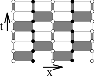
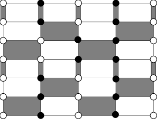
Figure 1: Two spin configurations in $(1+1)$ dimensions. The shaded plaquettes and time-like bonds carry the interaction. Filled dots represent spin up and open circles represent spin down. For an antiferromagnetic spin chain in a positive magnetic field $B_{x}>0$, the second configuration has $\mbox{Sign}[s]=-1$.

The central observable of our study is the uniform magnetization

$$M^{i}=\sum_{x}S_{x}^{i}.$$ (3.15)

The expectation value of the magnetization $\langle M^{1}\rangle$ in the direction of the magnetic field is non-zero, while $\langle M^{2}\rangle=\langle M^{3}\rangle=0$.

It should be noted that the path integral can be simplified for isotropic ferromagnets ($J^{\prime}=J<0$) or antiferromagnets ($J^{\prime}=J>0$) in a uniform magnetic field ($B_{x}=B$). In that case, the magnetic field interaction $B\sum_{x}S_{x}^{1}$ commutes with the rest of the Hamiltonian and can hence be concentrated in a single Euclidean time-step. Then one can work with only $2dM+1$ time-slices instead of $(2d+1)M$. Instead of $M$ magnetic field interaction time-steps with Boltzmann weights $\cosh(\epsilon B/2)$ and $\sinh(\epsilon B/2)$ one then has only one such step with Boltzmann weights $\cosh(\beta B/2)$ and $\sinh(\beta B/2)$. In the simulations performed in this paper we use the method with $(2d+1)M$ time-slices.

4 Cluster Algorithm for the Modified Model without the Sign Factor

The meron-cluster algorithm is based on a cluster algorithm for the modified model without the sign factor. Quantum spin systems without a sign problem can be simulated very efficiently with the loop-cluster algorithm [7, 8, 9]. This algorithm can be implemented directly in the Euclidean time continuum [10], i.e. the Suzuki-Trotter discretization is not even necessary. The same is true for the meron-cluster algorithm. Here we discuss the algorithm for discrete time.

The idea behind the algorithm is to decompose a configuration into clusters which can be flipped independently. Each lattice site belongs to exactly one cluster. When the cluster is flipped, the spins at all the sites on the cluster are changed from up to down and vice versa. The decomposition of the lattice into clusters results from connecting neighboring sites on each space-time interaction plaquette or time-like interaction bond according to probabilistic cluster rules. A set of connected sites defines a cluster. In this case the clusters are open or closed strings. The cluster rules are constructed so as to obey detailed balance. To show this property we first write the space-time plaquette Boltzmann factors as

$$\!\!\!\exp(-S[s(x,t),s(x+\hat{i},t),s(x,t+1),s(x+\hat{i},t+1)])=$$ (4.1)

$$\!\!\!A\delta_{s(x,t),s(x,t+1)}\delta_{s(x+\hat{i},t),s(x+\hat{i},t+1)}+B\delta_{s(x,t),-s(x+\hat{i},t)}\delta_{s(x,t+1),-s(x+\hat{i},t+1)}+$$

$$\!\!\!C\delta_{s(x,t),s(x,t+1)}\delta_{s(x+\hat{i},t),s(x+\hat{i},t+1)}\delta_{s(x,t),-s(x+\hat{i},t)}+D\delta_{s(x,t),s(x+\hat{i},t+1)}\delta_{s(x+\hat{i},t),s(x,t+1)}+$$

$$\!\!\!E\delta_{s(x,t),s(x,t+1)}\delta_{s(x+\hat{i},t),s(x+\hat{i},t+1)}\delta_{s(x,t),s(x+\hat{i},t)}.$$

The various $\delta$-functions specify which sites are connected and thus belong to the same cluster. It is possible to construct a cluster algorithm satisfying detailed balance if the coefficients $A,B,...,E$ are all non-negative. In that case these coefficients determine the relative probabilities for different cluster break-ups of an interaction plaquette. For example, $A$ determines the probability with which sites are connected with their time-like neighbors, while $B$ and $D$ determine the probabilities for connections with space-like and diagonal neighbors. The quantities $C$ and $E$ determine the probabilities to put all four spins of a plaquette into the same cluster. This is possible for plaquette configurations $[\uparrow,\downarrow,\uparrow,\downarrow]$ or $[\downarrow,\uparrow,\downarrow,\uparrow]$ with a probability proportional to $C$ and for configurations $[\uparrow,\uparrow,\uparrow,\uparrow]$ or $[\downarrow,\downarrow,\downarrow,\downarrow]$ with a probability proportional to $E$. Inserting the expressions from eq.(3) one finds

$$\exp(-S[\uparrow,\uparrow,\uparrow,\uparrow])=\exp(-S[\downarrow,\downarrow,\downarrow,\downarrow])=\exp(-\epsilon J^{\prime}/2)=A+D+E,$$

$$\exp(-S[\uparrow,\downarrow,\uparrow,\downarrow])=\exp(-S[\downarrow,\uparrow,\downarrow,\uparrow])=\cosh(\epsilon J/2)=A+B+C,$$

$$\exp(-S[\uparrow,\downarrow,\downarrow,\uparrow])=\exp(-S[\downarrow,\uparrow,\uparrow,\downarrow])=\sinh(\epsilon|J|/2)=B+D.$$ (4.2)

For example, the probability to connect the sites with their time-like neighbors on a plaquette with configuration $[\uparrow,\uparrow,\uparrow,\uparrow]$ or $[\downarrow,\downarrow,\downarrow,\downarrow]$ is $A/(A+D+E)$, while the probability to connect them with their diagonal neighbor is $D/(A+D+E)$. All sites on such a plaquette are connected together and are hence put into the same cluster with probability $E/(A+D+E)$. Similarly, the probability for connecting space-like neighbors on a plaquette with configuration $[\uparrow,\downarrow,\downarrow,\uparrow]$ or $[\downarrow,\uparrow,\uparrow,\downarrow]$ is $B/(B+D)$ and the probability for connecting diagonal neighbors is $D/(B+D)$. Similarly, the time-like bond Boltzmann factors are expressed as

$$\exp(-S[s(x,t),s(x,t+1)])=F\delta_{s(x,t),s(x,t+1)}+G.$$ (4.3)

The probability to connect spins with their time-like neighbors is $F/(F+G)$. The spins remain disconnected with probability $G/(F+G)$. Inserting the expressions from eq.(3) one obtains

$$\exp(-S[\uparrow,\uparrow])=\exp(-S[\downarrow,\downarrow])=\cosh(\epsilon B_{x}/2)=F+G,$$

$$\exp(-S[\uparrow,\downarrow])=\exp(-S[\downarrow,\uparrow])=\sinh(\epsilon|B_{x}|/2)=F.$$ (4.4)

The cluster rules are illustrated in table 1.

weight	configuration	break-ups
$\exp(-\epsilon J^{\prime}/2)$		A      D      E
$\cosh(\epsilon J/2)$		A      B      C
$\sinh(\epsilon|J|/2)$		B      D
$\cosh(\epsilon B_{x}/2)$		F                       G
$\sinh(\epsilon|B_{x}|/2)$		G

Table 1: Cluster break-ups of various plaquette and time-like bond configurations together with their relative probabilities $A,B,...,G$. Filled dots represent spin up, open circles represent spin down, and the fat lines are the cluster connections.

Eqs.(4.1,4.3) can be viewed as a representation of the original model as a random cluster model. The cluster algorithm operates in two steps. First, a cluster break-up is chosen for each space-time interaction plaquette or time-like interaction bond according to the above probabilities. This effectively replaces the original Boltzmann weight of a configuration with a set of constraints represented by the $\delta$-functions associated with the chosen break-up. The constraints imply that the spins in one cluster can only be flipped together. Second, every cluster is flipped with probability $1/2$. When a cluster is flipped, the spins on all sites that belong to the cluster are flipped from up to down and vice versa. Eqs.(4,4) ensure that the cluster algorithm obeys detailed balance. To determine $A,B,...,E$ we distinguish three cases. For $J^{\prime}>J>0$ we solve eq.(4) by

$$A=\exp(-\epsilon J^{\prime}/2),\ B=\sinh(\epsilon J/2),\ C=\exp(-\epsilon J/2)-\exp(-\epsilon J^{\prime}/2),\ D=E=0.$$ (4.5)

For $-J\leq J^{\prime}\leq J$ we use

$$A=\frac{1}{2}[\exp(-\epsilon J^{\prime}/2)+\exp(-\epsilon J/2)],\ B=\frac{1}{2}[\exp(\epsilon J/2)-\exp(-\epsilon J^{\prime}/2)],\ C=0,$$

$$D=\frac{1}{2}[\exp(-\epsilon J^{\prime}/2)-\exp(-\epsilon J/2)],\ E=0,$$ (4.6)

and for $J^{\prime}\leq J<0$

$$A=\cosh(\epsilon J/2),\ B=C=0,\ D=\sinh(\epsilon|J|/2),\ E=\exp(-\epsilon J^{\prime}/2)-\exp(\epsilon|J|/2).$$ (4.7)

For example, for the antiferromagnetic quantum Heisenberg model ($J^{\prime}=J>0$) we have

$$A=\exp(-\epsilon J/2),\,B=\sinh(\epsilon J/2),\,C=D=E=0.$$ (4.8)

Consequently, on plaquette configurations $[\uparrow,\uparrow,\uparrow,\uparrow]$ or $[\downarrow,\downarrow,\downarrow,\downarrow]$ one always chooses time-like connections between the sites, and for configurations $[\uparrow,\downarrow,\downarrow,\uparrow]$ or $[\downarrow,\uparrow,\uparrow,\downarrow]$ one always chooses space-like connections. For configurations $[\uparrow,\downarrow,\uparrow,\downarrow]$ or $[\downarrow,\uparrow,\downarrow,\uparrow]$ one chooses time-like connections with probability $p=A/(A+B)=2/[1+\exp(\epsilon J)]$ and space-like connections with probability $1-p=B/(A+B)$. Similarly, eq.(4) yields

$$F=\exp(-\epsilon|B_{x}|/2),\,G=\sinh(\epsilon|B_{x}|/2).$$ (4.9)

The above cluster rules were first used in a simulation of the Heisenberg antiferromagnet [8] in the absence of a magnetic field. In that case there is no sign problem. Then the corresponding loop-cluster algorithm is extremely efficient and has almost no detectable autocorrelations. When a magnetic field is switched on the situation changes. When the magnetic field points in the direction of the spin quantization axis (the $3$-direction in our case) there is no sign problem. However, the magnetic field then explicitly breaks the ${\sf Z\!\!\!Z}(2)$ flip symmetry on which the cluster algorithm is based, and the clusters can no longer be flipped with probability $1/2$. Instead the flip probability is determined by the value of the magnetic field and by the magnetization of the cluster. When the field is strong, flips of magnetized clusters are rarely possible and the algorithm becomes very inefficient. To avoid this problem, we have chosen the magnetic field to point in the $1$-direction, i.e. perpendicular to the spin quantization axis. In that case, the cluster flip symmetry is not affected by the magnetic field, and the clusters can still be flipped with probability $1/2$. However, in several cases one now has a sign problem and the cluster algorithm becomes extremely inefficient again. Fortunately, using the meron concept the sign problem can be eliminated completely and the efficiency of the original cluster algorithm can be maintained even in the presence of a magnetic field.

5 Meron-Clusters and the Sign Problem

Let us consider the effect of a cluster flip on the sign. As discussed before, the flip of a meron-cluster changes $\mbox{Sign}[s]$, while the flip of a non-meron-cluster leaves $\mbox{Sign}[s]$ unchanged. An example of a meron-cluster is shown in figure 2 along with the same spin configurations as in figure 1. When the meron cluster is flipped the first configuration with $\mbox{Sign}[s]=1$ turns into the second configuration with $\mbox{Sign}[s]=-1$. This property of the cluster is independent of the orientation of any other cluster. Since flipping all spins leaves $\mbox{Sign}[s]$ unchanged, the total number of meron-clusters is always even.

                        ${\rm Sign[s]}=1$                                             ${\rm Sign[s]}=-1$

         

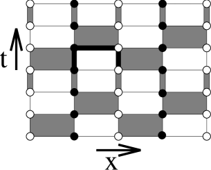
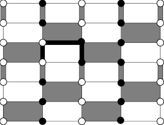
Figure 2: The same spin configurations as in figure 1 together with a meron-cluster represented by the fat black line. The other clusters are not shown. Flipping the meron-cluster changes one configuration into the other and changes $\mbox{Sign}[s]$.

The meron concept allows us to gain an exponential factor in statistics. Since all clusters can be flipped independently with probability $1/2$, one can construct an improved estimator for $\langle\mbox{Sign}\rangle$ by averaging analytically over the $2^{N_{C}}$ configurations obtained by flipping the $N_{C}$ clusters in a configuration in all possible ways. For configurations that contain merons, the average $\mbox{Sign}[s]$ is zero because flipping a single meron-cluster leads to a cancellation of contributions $\pm 1$. Hence only the configurations without merons contribute to $\langle\mbox{Sign}\rangle$. The probability to have a configuration without merons is equal to $\langle\mbox{Sign}\rangle$ and is hence exponentially suppressed with the space-time volume. The vast majority of configurations contains merons and contributes an exact $0$ to $\langle\mbox{Sign}\rangle$ instead of a statistical average of contributions $\pm 1$. In this way the improved estimator leads to an exponential gain in statistics.

Now we want to show that the contributions from the zero-meron sector are always positive. With no merons in the configuration it is clear that the sign remains unchanged under cluster flips, but it is not obvious that one always has $\mbox{Sign}[s]=1$. To prove this we note that there is no sign problem in the absence of the magnetic field. In that case all configurations have $\mbox{Sign}[s]=1$ and all clusters are closed loops. In the presence of the magnetic field some of the closed loops are cut into open string pieces. However, one can always flip the individual pieces such that a typical configuration of the model without the magnetic field emerges. These reference configurations have $\mbox{Sign}[s]=1$. Since any configuration can be turned into such a configuration by cluster flips, and since the sign remains unchanged when a non-meron-cluster is flipped, all configurations without merons have $\mbox{Sign}[s]=1$. At this point we have solved one half of the sign problem.

Before we can solve the other half of the problem we must discuss the improved estimator for the magnetization. Since the magnetization operator $M^{1}=\sum_{x}S^{1}_{x}$ is not diagonal in the basis we have chosen to quantize the spins (which is along the $3$-direction), it is not obvious how to measure it. However, as discussed in [22], quantum cluster algorithms naturally allow us to measure non-diagonal operators. In the present case, due to time translation invariance, $M^{1}$ is equivalent to a sum of local spin-flip operators $S_{x}^{1}$ inserted at any time slice and appropriately averaged. An open string cluster that contains the point $(x,t)$ is naturally divided into two parts, one on each side of the point. Flipping each side while keeping the other side fixed produces spin configurations that contribute to the spin flip operator $S_{x}^{1}$ at time $t$. Closed loop-clusters, on the other hand, do not decompose into two parts and thus do not contribute to this operator. If we construct an improved estimator for $S_{x}^{1}$ inserted at the time $t$, a configuration containing more than one meron does not contribute to $\langle S_{x}^{1}\rangle$. Since the total number of merons is always even, in there exists at least one meron that does not contain the point $(x,t)$. Flipping that meron changes the sign but not $S_{x}^{1}$ and hence results in an exact cancellation of two equal and opposite contributions to $\langle S_{x}^{1}\rangle$. Hence we can focus entirely on the zero-meron sector. In this sector the point $(x,t)$ can divide an open string cluster into two merons or two non-merons. When both parts are non-merons, flipping one part but not the other yields a contribution of $1/2$ to $\langle S_{x}^{1}\rangle$. When both parts are merons, on the other hand, one gets a contribution of $-1/2$. Summing over $x,t$ one obtains $\langle M^{1}\rangle$.

For an antiferromagnet in a uniform magnetic field $B_{x}=B$, one can find a simple expression for the improved estimator for $\langle M^{1}\rangle$ in terms of a winding number of closed loops which result from joining the open string clusters. In that case a non-meron cluster has the property that both end points of an open string cluster have the same spin type, either up or down. If all the open string clusters are flipped into a reference configuration and joined together to form closed loops, one can define $W_{l}$ for each loop to be the temporal winding number of the loop. We assume that the cluster is growing in the positive direction on the sites where the loop is broken into open strings. Since the loop is always broken up on the same type of spin, the above definition of the winding of a given loop is consistent. Further, if a particular loop is not composed of open string clusters then $W_{l}=0$. With this definition of $W_{l}$ it is easy to show that

$$\langle M^{1}\rangle=\frac{\langle\delta_{N,0}\sum_{l}W_{l}\rangle}{2\langle\delta_{N,0}\rangle},$$ (5.1)

where $N$ is the number of meron-clusters. Hence, as explained above, the magnetization gets non-vanishing contributions only from the zero-meron sector. One should note that $W_{l}$ can be negative.

Since the magnetization gets non-vanishing contributions only from the zero-meron sector, it is unnecessary to generate any configuration that contains meron-clusters. This observation is the key to the solution of the other half of the sign problem. In fact, one can gain an exponential factor in statistics by restricting the simulation to the zero-meron sector, which represents an exponentially small fraction of the whole configuration space. This procedure enhances both the numerator and the denominator in eq.(5.1) by a factor that is exponentially large in the volume, but leaves the ratio of the two invariant. In practice, it is advantageous to occasionally generate configurations containing merons even though they do not contribute to our observable, because this reduces the autocorrelation times. Still, in order to solve the sign problem multi-meron configurations must be very much suppressed. To suppress such configurations in a controlled way, we introduce an additional Boltzmann factor $q<1$ for each meron, which determines the relative weights of the $N$-meron sectors. We visit all plaquette and time-like bond interactions one after the other and choose new pair connections between the sites according to the above cluster rules. The suppression factor $q$ is used in a Metropolis accept-reject step. A newly proposed pair connection that changes the number of merons from $N$ to $N^{\prime}$ is accepted with probability $p=\mbox{min}[1,q^{N^{\prime}-N}]$. It should be stressed that adding the Boltzmann factor for the reweighting doesn’t change the physics, only the algorithm. After visiting all plaquette and time-like bond interactions, each cluster is flipped with probability $1/2$ which completes one update sweep. After reweighting, multi-meron configurations are very much suppressed. This completes the second step in our solution of the sign problem.

6 Antiferromagnetic Spin Ladders in a Uniform Magnetic Field

Antiferromagnetic spin ladders — sets of several transversely coupled quantum spin chains — are interesting condensed matter systems which interpolate between single 1-d spin chains and 2-d quantum antiferromagnets. The ladders are spatially quasi 1-d systems whose low-energy dynamics are governed by $(1+1)$-d quantum field theories, which can be solved analytically using Bethe ansatz techniques. This allows us to test field theoretical predictions for such models using condensed matter experiments as well as numerical simulations. Here we consider spin ladders in an external uniform magnetic field $B_{x}=B$, which corresponds to a chemical potential $\mu=B/c$ in the corresponding $(1+1)$-d quantum field theory. The Bethe ansatz solution of this theory yields predictions for the magnetization of the ladder system, which we compare with results of numerical simulations.

Haldane was first to realize the connection between spin chains and $(1+1)$-d field theories [15]. He conjectured that a single 1-d antiferromagnetic quantum spin chain of length $L$ at inverse temperature $\beta$ is described by a $(1+1)$-d $O(3)$ symmetric quantum field theory with an action

$$S[\vec{e}]=\int_{0}^{\beta}dt\int_{0}^{L}dx\ [\frac{c}{2g^{2}}(\partial_{x}\vec{e}\cdot\partial_{x}\vec{e}+\frac{1}{c^{2}}\partial_{t}\vec{e}\cdot\partial_{t}\vec{e})+\frac{i\theta}{4\pi}\vec{e}\cdot(\partial_{x}\vec{e}\times\partial_{t}\vec{e})].$$ (6.1)

Here $\vec{e}(x,t)$ is a three-component unit-vector field, $g$ is a coupling constant and $c$ is the spin-wave velocity. The vacuum angle is given by $\theta=2\pi S$, where $S$ is the value of the spin, hence quantum spin chains with integer spin have $\theta=0$ and chains with half-integer spin have $\theta=\pi$. The $(1+1)$-d $O(3)$ model is an asymptotically free quantum field theory with a non-perturbatively generated mass-gap $m\propto\exp(-2\pi/g^{2})$ at $\theta=0$. At $\theta=\pi$, on the other hand, the mass-gap disappears. This naturally explains why chains of half-integer spins are gapless, while chains of integer spins have a gap. For large values of the spin $S$ the coupling constant is given by $1/g^{2}=S/2$, so the mass-gap $m\propto\exp(-\pi S)$ goes to zero and the system approaches a continuum limit.

Chakravarty, Halperin and Nelson used a $(2+1)$-d effective field theory to describe the low-energy dynamics of spatially 2-d quantum antiferromagnets [23]. Chakravarty has applied this theory to quantum spin ladders with a large even number of coupled spin $1/2$ chains [21]. We consider spin ladders with the same value of the antiferromagnetic coupling along and between the chains. These systems are described by the action

$$S[\vec{e}]=\int_{0}^{\beta}dt\int_{0}^{L}dx\int_{0}^{L^{\prime}}dy\ \frac{\rho_{s}}{2}[\partial_{x}\vec{e}\cdot\partial_{x}\vec{e}+\partial_{y}\vec{e}\cdot\partial_{y}\vec{e}+\frac{1}{c^{2}}\partial_{t}\vec{e}\cdot\partial_{t}\vec{e}],$$ (6.2)

where $\rho_{s}$ is the spin stiffness and $c$ is the spin-wave velocity. The coupled spin chains are oriented in the spatial $x$-direction with a large extent $L$, while the transverse $y$-direction has a much smaller extent $L^{\prime}\ll L$. Here we consider spin ladders with periodic boundary conditions in the transverse direction, and we limit ourselves to an even number of coupled spin $1/2$ chains. The effective action for a ladder with an odd number of coupled chains would contain an additional topological term.

When the spin ladder is placed in a uniform external magnetic field $\vec{B}$, the field couples to a conserved quantity — the uniform magnetization. Hence, on the level of the effective theory, the magnetic field plays the role of a chemical potential, i.e. it appears as the time-component of an imaginary constant vector potential. As a consequence, the ordinary derivative $\partial_{t}\vec{e}$ is replaced by the covariant derivative $\partial_{t}\vec{e}+i\vec{B}\times\vec{e}$ and the effective action takes the form

$$S[\vec{e}]=\int_{0}^{\beta}dt\int_{0}^{L}dx\int_{0}^{L^{\prime}}dy\ \frac{\rho_{s}}{2}[\partial_{x}\vec{e}\cdot\partial_{x}\vec{e}+\partial_{y}\vec{e}\cdot\partial_{y}\vec{e}+\frac{1}{c^{2}}(\partial_{t}\vec{e}+i\vec{B}\times\vec{e})\cdot(\partial_{t}\vec{e}+i\vec{B}\times\vec{e})].$$ (6.3)

For a sufficiently large even number of coupled chains ($L^{\prime}\gg c/\rho_{s}$) the ladder system undergoes dimensional reduction to the $(1+1)$-d $O(3)$ symmetric quantum field theory with the action

$$S[\vec{e}] = \int_{0}^{\beta}dt\int_{0}^{L}dx\ \frac{\rho_{s}L^{\prime}}{2}[\partial_{x}\vec{e}\cdot\partial_{x}\vec{e}+\frac{1}{c^{2}}(\partial_{t}\vec{e}+i\vec{B}\times\vec{e})\cdot(\partial_{t}\vec{e}+i\vec{B}\times\vec{e})]$$ (6.4)

$$= \int_{0}^{\beta c}dct\int_{0}^{L}dx\ \frac{1}{2g^{2}}[\partial_{x}\vec{e}\cdot\partial_{x}\vec{e}+(\partial_{ct}\vec{e}+i\vec{\mu}\times\vec{e})\cdot(\partial_{ct}\vec{e}+i\vec{\mu}\times\vec{e})].$$

The effective coupling constant is given by $1/g^{2}=\rho_{s}L^{\prime}/c$ and the magnetic field appears as a chemical potential of magnitude $\mu=B/c$.

The $(1+1)$-d $O(3)$ model with chemical potential $\mu$ has been solved exactly by Wiegmann [24] using Bethe ansatz techniques. Using this solution, Hasenfratz, Maggiore and Niedermayer have derived an exact result for the non-perturbatively generated mass-gap $m$ in this model [25]. In particular, for $\mu\geq m$ and $\beta=L=\infty$ the Bethe ansatz yields the free energy density

$$f(\mu)-f(0)=-\frac{1}{2\pi}\int_{-\theta_{0}}^{\theta_{0}}d\theta\epsilon(\theta)m\cosh\theta,$$ (6.5)

where the function $\epsilon(\theta)$ satisfies the integral equation

$$\epsilon(\theta)-\int_{-\theta_{0}}^{\theta_{0}}d\theta^{\prime}\frac{\epsilon(\theta^{\prime})}{(\theta^{\prime}-\theta)^{2}+\pi^{2}}=\mu-m\cosh\theta,$$ (6.6)

and $\theta_{0}$ is defined by the boundary condition $\epsilon(\pm\theta_{0})=0$. For $\mu<m$ no particles can be produced and $f(\mu)=f(0)$. For chemical potentials slightly above this threshold the previous equations imply

$$f(\mu)-f(0)=-\frac{2}{3}\frac{\sqrt{2m}}{\pi}(\mu-m)^{3/2}$$ (6.7)

and the resulting particle density is given by

$$\frac{\langle N\rangle}{L}=-\frac{df(\mu)}{d\mu}=\frac{\sqrt{2m}}{\pi}\sqrt{\mu-m}.$$ (6.8)

This quantum field theoretic result can be translated back into the language of condensed matter physics. It yields an expression for the magnetization density

$$\frac{\langle M^{1}\rangle}{L}=\frac{\sqrt{2m}}{\pi}\sqrt{\frac{B}{c}-m}$$ (6.9)

as a function of the magnetic field $B$. The square root form was derived earlier in [28]. Our result yields an explicit expression for the prefactor as well.

In the next chapter we will present results of numerical simulations using the meron-cluster algorithm. The numerical results are obtained at small but non-zero temperatures and for ladders of large but finite lengths, while the above analytic expressions are for $\beta=L=\infty$. In particular, the results in the threshold region $\mu\approx m$ are very sensitive to finite-size and finite-temperature effects. Fortunately, these effects can still be understood analytically. In particular, the Bethe ansatz solution reveals that for not too large $\mu$ the system is equivalent to a dilute gas of fermions. Its magnetization density is hence given by

$$\frac{\langle M^{1}\rangle}{L}=\frac{1}{L}\sum_{n\in{\sf Z\!\!\!Z}}[1+\exp(\beta(c\sqrt{(\frac{2\pi n}{L})^{2}+m^{2}}-B))]^{-1}.$$ (6.10)

Up to this point we have considered the mass-gap $m$ as an unknown constant. Based on results from [23, 25, 26], Chakravarty [21] has expressed the mass-gap of the ladder system as

$$m=\frac{16\pi\rho_{s}}{ec}\exp(-2\pi\rho_{s}L^{\prime}/c)[1+\frac{c}{4\pi\rho_{s}L^{\prime}}+{\cal O}((\frac{c}{\rho_{s}L^{\prime}})^{2})].$$ (6.11)

For the spin $1/2$ quantum Heisenberg model with exchange coupling $J$ on a 2-d lattice of spacing $a$, the values of the spin stiffness $\rho_{s}=0.1800(5)J$ and the spin-wave velocity $c=1.657(2)Ja$ are known from very precise cluster algorithm simulations [27]. As discussed in [27], the above expression for the mass-gap is expected to be accurate for a sufficiently large number $L^{\prime}/a>12$ of coupled chains. The simulations in the present paper are performed at $L^{\prime}/a=4$ and are thus not expected to be described accurately by this formula. Still, for $L^{\prime}/a=4$ the value $m=0.141(2)/a$ is known from the simulations of [20].

There is another interesting phenomenon that occurs at rather large values of the magnetic field, namely saturation of the magnetization — all spins follow the external field and the system becomes completely ferromagnetically ordered. This effect cannot be understood in the framework of the above low-energy effective theory because it assumes antiferromagnetic order. Still, it is easy to convince oneself that there must be a critical magnetic field beyond which saturation occurs. This effect is indeed observed in the numerical simulations described below.

7 Numerical Results

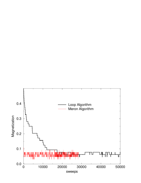
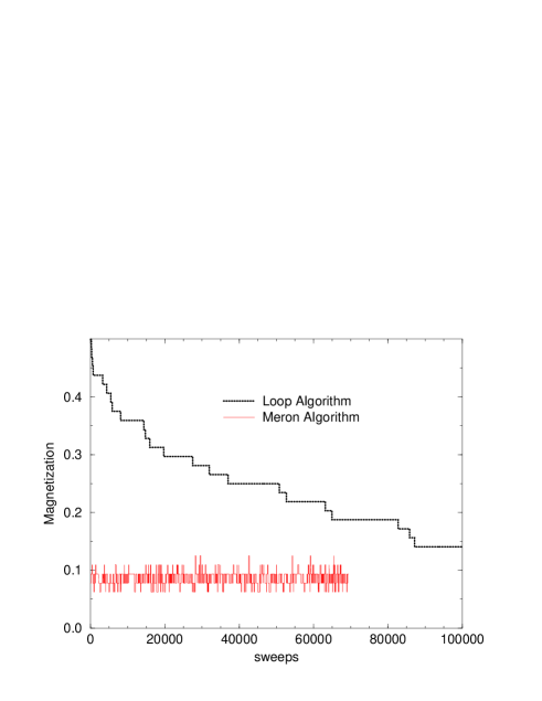
Figure 3: Thermalization of the magnetization for the loop-cluster algorithm versus the meron-cluster algorithm. The first graph is for a magnetic field $B=0.75J$ and the second graph is for $B=J$. For $B=J$ the loop algorithm takes more than 100000 sweeps to reach equilibrium while the meron-cluster algorithm has no thermalization problem.

We have performed numerical simulations with the meron-cluster algorithm for various quantum antiferromagnets in a uniform magnetic field $B$. To demonstrate the efficiency of the algorithm, we have compared it with the standard loop-cluster algorithm. In case of the loop algorithm, the magnetic field points in the direction of the spin quantization axis. Hence the ${\sf Z\!\!\!Z}(2)$ symmetry that allows the clusters to be flipped with probability $1/2$ at $B=0$ is explicitly broken by the magnetic field. In this case some loop-clusters can be flipped only with very small probability and the algorithm becomes inefficient for large values of $B$. In the meron-cluster algorithm, on the other hand, the magnetic field is perpendicular to the spin quantization axis and all clusters can still be flipped with probability $1/2$. Now the sign problem arises, but it is solved completely by the meron-cluster algorithm. Figure 3 compares the thermalization behavior of the magnetization of a 2-d Heisenberg antiferromagnet on an $8\times 8$ lattice at $\beta J=10$ with $M=100$ for the loop-cluster algorithm and the meron-cluster algorithm. At $B=0.75J$, the loop-cluster algorithm takes about 20000 sweeps until thermal equilibrium is reached, while the meron-cluster algorithm equilibrates much faster. At $B=J$, the loop-cluster algorithm already needs more than 100000 equilibration sweeps, but the meron-cluster algorithm again has no thermalization problem. It should be pointed out that the loop-cluster algorithm works reasonably well for small values of $B$ and has been used in an interesting numerical study in [29]. However, for larger values of $B$ the meron-cluster algorithm is clearly superior. It would be interesting to compare the performance of the meron-cluster algorithm with that of the worm algorithm [11, 12] and the stochastic series expansion technique [13].

Some of our data for the magnetization density $\langle M^{1}\rangle a/L$ of 2-d antiferromagnetic spin systems on an $L/a\times L^{\prime}/a$ lattice at inverse temperature $\beta$ are contained in table 2.

$L/a$	$L^{\prime}/a$	$\beta J$	$M$	$B/J$	$\langle M^{1}\rangle a/L$
8	8	10	100	0.75	0.488(6)
8	8	10	100	1.00	0.690(6)
20	4	15	200	0.10	0.0048(4)
20	4	15	200	0.20	0.0184(4)
20	4	15	200	0.30	0.0452(8)
20	4	15	200	0.40	0.086(2)
20	4	15	200	0.50	0.120(4)
20	4	15	200	1.00	0.324(4)
20	4	15	200	2.00	0.76(2)
20	4	15	200	3.00	1.280(8)
20	4	15	200	4.00	1.93(3)
20	4	15	200	4.20	2.000(8)
20	4	15	200	4.40	2.000(8)
40	4	24	300	0.10	0.00104(8)
40	4	24	300	0.20	0.0096(6)
40	4	24	300	0.30	0.042(2)
40	4	24	300	0.40	0.085(3)
40	4	24	300	0.50	0.117(7)
40	4	24	300	1.00	0.332(4)

Table 2: Numerical results for the magnetization density $\langle M^{1}\rangle a/L$ for various spatial sizes $L,L^{\prime}$, inverse temperatures $\beta$, Trotter numbers $M$ and magnetic field values $B$.

Figure 4: The probability of having a certain number of merons for various values of the magnetic field $B/J=0.01,0.05,0.2$ and $0.3$.

Figure 4 shows the probability to have a certain number of merons in an algorithm that samples all meron-sectors without reweighting. This calculation was done on an $8\times 8$ lattice at $\beta J=1$ and $M=100$. For small values of $B$ the zero-meron sector and hence $\langle\mbox{Sign}\rangle$ are relatively large, while multi-meron configurations are rare. On the other hand, for larger values of the magnetic field the vast majority of configurations have a large number of merons and hence $\langle\mbox{Sign}\rangle$ is exponentially small. The meron-cluster algorithm suppresses the multi-meron configurations and concentrates on the zero-meron sector which is the only one that contributes to the magnetization.

Figure 5: Magnetization density $\langle M^{1}\rangle/L$ of quantum spin ladders consisting of $L^{\prime}/a=4$ coupled chains as a function of the magnetic field $B$. The numerical data are for two systems: one of size $L/a=20$ at inverse temperature $\beta J=15$ (circles) and the other for $L/a=40$ at $\beta J=24$ (diamonds). The solid curve is the infinite volume, zero temperature analytic result, while the two dashed curves are finite volume, non-zero temperature analytic results for the two simulated systems in the small $B$ region. The dotted curve represents saturation of the magnetization per spin at $1/2$.

Figure 5 shows the magnetization density of antiferromagnetic quantum spin ladders consisting of four coupled spin $1/2$ chains (i.e. $L^{\prime}/a=4$). The cases $L/a=20,\beta J=15,M=200$ and $L/a=40,\beta J=24,M=300$ have been investigated. Within our statistical errors these Trotter numbers give results indistinguishable from the time-continuum limit. In any case, following [10] it would be straightforward to implement the meron-cluster algorithm directly in the Euclidean time continuum. Using the values $m=0.141(2)/a$ from [20] and $c=1.657(2)Ja$ from [27], the finite volume, non-zero temperature expression of eq.(6.10) that was derived for small values of $B$ (represented by the dashed curves in figure 5) describes the data rather well in that regime. Using the same values for $m$ and $c$, the infinite volume, zero temperature expression for $\langle M^{1}\rangle/L$ that results from solving eqs.(6.5) and (6.6) (represented by the solid curve in figure 5) is in good agreement with the numerical data for intermediate values of $B$. For $B/c$ slightly above the threshold $m$, the infinite volume, zero temperature expression for $\langle M^{1}\rangle/L$ is given by eq.(6.9). In the threshold region finite size and finite temperature effects are rather large and our numerical data do not fall in the applicability range of eq.(6.9). As expected, for large values of $B$ the magnetization per spin saturates at $1/2$ (represented by the dotted curve in figure 5). Note that $\langle M^{1}\rangle a/L=2$ for $L^{\prime}/a=4$ in table 2 corresponds to a value $\langle M^{1}\rangle a^{2}/(LL^{\prime})=1/2$ per spin. It should be stressed that the comparison of analytic and numerical results does not involve any adjustable parameters. Of course, one should not expect perfect agreement. Given the fact that the simulations were performed at $L^{\prime}/a=4$ while the analytic expressions were derived in the large $L^{\prime}/a$ limit, the agreement between theory and numerical data is quite remarkable.

8 Conclusions

Antiferromagnetic quantum spin systems in a uniform external magnetic field $B$ are very difficult to simulate numerically. For example, the standard loop-cluster algorithm, which is very efficient for $B=0$, suffers from exponential slowing down for large values of the field. Here we have traded this slowing down problem for a severe sign problem by a change of the spin quantization axis. Meron-cluster algorithms provide a general strategy to deal with sign problems and have previously led to a complete solution of severe fermion sign problems [1, 2, 3, 4]. Here we have generalized the meron concept to quantum spins in a magnetic field, which again led to a complete solution of the sign problem for these bosonic systems. Our numerical simulations of quantum spin ladders are in agreement with analytic predictions and confirm that ladders consisting of an even number of transversely coupled spin $1/2$ chains are described by a $(1+1)$-d $O(3)$ symmetric quantum field theory.

In conclusion, the meron concept provides us with a powerful algorithmic tool — the meron-cluster algorithm — which can lead to a complete solution of severe sign problems. In this paper we have demonstrated that this algorithm allows us to simulate bosonic quantum spin systems in an arbitrary magnetic field. The next challenge is to construct meron-cluster algorithms for systems that show high-temperature superconductivity. A first step in this direction was taken in [4]. In that paper a Hamiltonian with the symmetries of the Hubbard model but with enhanced antiferromagnetic couplings has been investigated. The enhanced antiferromagnetic couplings allowed us to solve the fermion sign problem in that model. It turned out that after doping the model undergoes phase separation and does not superconduct. It remains to be seen if meron-cluster algorithms can also be constructed for models that show high-temperature superconductivity.

References

- [1] S. Chandrasekharan and U.-J. Wiese, cond-mat/9902128.
- [2] S. Chandrasekharan, J. Cox, K. Holland and U.-J. Wiese, hep-lat/9906021.
- [3] S. Chandrasekharan, hep-lat/9909007.
- [4] J. Cox, C. Gattringer, K. Holland, B. Scarlet and U.-J. Wiese, hep-lat/9909119.
- [5] W. Bietenholz, A. Pochinsky and U.-J. Wiese, Phys. Rev. Lett. 75 (1995) 4524.
- [6] U.-J. Wiese and H.-P. Ying, Phys. Lett. A168 (1992) 143.
- [7] H. G. Evertz, G. Lana and M. Marcu, Phys. Rev. Lett. 70 (1993) 875.
- [8] U.-J. Wiese and H.-P. Ying, Z. Phys. B93 (1994) 147.
- [9] H. G. Evertz, The loop algorithm, in Numerical Methods for Lattice Quantum Many-Body Problems, ed. D. J. Scalapino, Addison-Wesley Longman, Frontiers in Physics
- [10] B. B. Beard and U.-J. Wiese, Phys. Rev. Lett. 77 (1996) 5130.
- [11] N. V. Prokof’ev, B. V. Svistunov and I. S. Tupitsyn, Pis’ma Zh. Eksp. Teor. Fiz. 64 (1996) 853 [JETP Lett. 64 (1996) 911]; Phys. Lett. A238 (1998) 253; JETP Lett. 87 (1998) 318.
- [12] V. A. Kashurnikov, N. V. Prokof’ev, B. V. Svistunov and M. Troyer, Phys. Rev. B59 (1999) 1162.
- [13] A. W. Sandvik, Phys. Rev. B59 (1999) R14157.
- [14] E. Dagotto and T. M. Rice, Science 271 (1996) 618.
- [15] F. D. M. Haldane, Phys. Rev. Lett. 50 (1983) 1153.
- [16] D. V. Khveshchenko, Phys. Rev. B50 (1994) 380.
- [17] S. R. White, R. M. Noack and D. J. Scalapino, Phys. Rev. Lett. 73 (1994) 886.
- [18] G. Sierra, J. Phys. A29 (1996) 3299.
- [19] M. Greven, R. J. Birgeneau and U.-J. Wiese, Phys. Rev. Lett. 77 (1996) 1865.
- [20] O. F. Syljuasen, S. Chakravarty and M. Greven, Phys. Rev. Lett. 78 (1997) 4115.
- [21] S. Chakravarty, Phys. Rev. Lett. 77 (1996) 4446.
- [22] R. Brower, S. Chandrasekharan and U.-J. Wiese, Physica A261 (1998) 520.
- [23] S. Chakravarty, B. I. Halperin and D. R. Nelson, Phys. Rev. Lett. 60 (1988) 1057; Phys. Rev. B39 (1989) 2344.
- [24] P. B. Wiegmann, Phys. Lett. B152 (1985) 209.
- [25] P. Hasenfratz, M. Maggiore and F. Niedermayer, Phys. Lett. B245 (1990) 522.
- [26] P. Hasenfratz and F. Niedermayer, Phys. Lett. B268 (1991) 231.
- [27] B. B. Beard, R. J. Birgeneau, M. Greven and U.-J. Wiese, Phys. Rev. Lett. 80 (1998) 1742.
- [28] R. Chitra and T. Giamarchi, Phys. Rev. B55 (1997) 5816.
- [29] M. Troyer and S. Sachdev, Phys. Rev. Lett. 81 (1998) 5418.