Path Integral Monte Carlo Simulations for Fermion Systems:
Pairing in the Electron-Hole Plasma.

Abstract

We review the path integral method wherein quantum systems are mapped with Feynman’s path integrals onto a classical system of “ring-polymers” and then simulated with the Monte Carlo technique. Bose or Fermi statistics correspond to possible “cross-linking” of polymers. As proposed by Feynman, superfluidity and Bose condensation result from macroscopic exchange of bosons. To map fermions onto a positive probability distribution, one must restrict the paths to lie in regions where the fermion density matrix is positive. We discuss a recent application to the two-component electron-hole plasma. At low temperature excitons and bi-excitons form. We have used nodal surfaces incorporating paired fermions and see evidence of a Bose condensation in the energy, specific heat and superfluid density. In the restricted path integral picture, pairing appears as intertwined electron-hole paths. Bose condensation occurs when these intertwined paths wind around the periodic boundaries.

1 INTRODUCTION

As first shown by Feynman [2], the thermodynamics of a quantum many-body system can be investigated using classical-statistical methods on polymer-like systems. To do this, one writes the density matrix of a many-body system at a temperature $k_{B}T=\beta^{-1}$ as an integral over all paths $\{R_{t}\}$:

$$\rho(R_{0},R_{\beta};\beta)=\frac{1}{N!}\sum_{\mathcal{P}}(\pm 1)^{\mathcal{P}}\oint_{\mathcal{P}R_{0}\rightarrow R_{\beta}}dR_{t}\exp(-S[R_{t}]).$$ (1)

The path $R(t)$ begins at $\mathcal{P}R_{0}$ and ends at $R_{\beta}$, and $\mathcal{P}$  is a permutation of particle labels. For $N$ particles, the path is in $3N$ dimensional space: $R_{t}=(\mathbf{r}_{1t},\mathbf{r}_{2t}\ldots\mathbf{r}_{Nt})$. The upper sign is to be used for bosons and the lower sign for fermions. For nonrelativistic particles interacting with a potential $V(R)$, the action of the path, $S[R_{t}]$, is given by:

$$S[R_{t}]=\int_{0}^{\beta}dt\left[\frac{m}{2}\left|\frac{dR_{t}}{\hbar dt}\right|^{2}+V(R_{t})\right].$$ (2)

Thermodynamic properties, such as the energy, are related to the diagonal part of the density matrix, so that the path returns to its starting place or to a permutation $\mathcal{P}$  of its starting place after a “time” $\beta$.

Since the imaginary-time action $S[R_{t}]$ is a real function of the path, for boltzmannons or bosons the integrand is nonnegative, and can be interpreted as a probability of an equivalent classical system and the action as the classical potential energy of a “polymer.” To perform Monte Carlo calculations of the integrand, one makes imaginary time discrete, so that one has a finite number of time slices and thereby a classical system of $N$ particles in $M$ time slices. If the path integral is performed by a simulation method, such as a generalization of Metropolis Monte Carlo or with molecular dynamics, one can obtain essentially exact results for problems such as the properties of liquid ⁴He at temperatures near the superfluid phase transition [3].

In addition to sampling the path, the permutation is also sampled. This is equivalent to allowing the ring polymers to connect in different ways. This macroscopic “percolation” of the polymers is directly related to superfluidity [2]. Superfluid behavior can occur at low temperature when the probability of exchange cycles on the order of the system size is nonnegligible. For details see Ref. [3].

However, the straightforward application of those techniques to Fermi systems means that odd permutations subtract from the integrand. The calculation of any physical operator by direct fermion PIMC is very inefficient because of the cancellation of positive and negative permutations. This is the “fermion sign problem.” Path integral methods as rigorous and successful as those for boson systems are not yet known for fermion systems in spite of the activities of many scientists throughout the last four decades.

2 RESTRICTED PATH INTEGRALS

For the diagonal density matrix we can arrange things so that we only get positive contributions by restricting the paths. We now sketch the derivation of the restricted path identity: that the nodes of the exact fermion many-body density matrix determine the rule by which one can take only paths with the same sign. The nodes of the fermion density matrix $\rho_{F}(R,R_{*};t)$ carve up space-time into a finite number of nodal cells defined as follows: call a node-avoiding path, a continuous path $R_{t}$ for $0<t\leq\beta$ for which $\rho_{F}(R_{t},R_{*};t)\neq 0$ for all $0<t<\beta$. Two points are in the same nodal cell if they are connected by a node-avoiding path (with respect to the same fixed $R_{*}$). The collection of all space time points $(R,t)$ connected by some node-avoiding path make up a nodal cell. Then we can solve the Bloch equation inside each nodal cell separately by specifying the initial conditions at $t=0$ and zero boundary conditions on the surface of the nodal cell. To enforce the zero boundary conditions, we insert an infinite repulsive potential precisely at the nodal surfaces which eliminates the contribution of any walks which hit or cross the node. Thus:

$$\rho_{F}(R_{\beta},R_{*};\beta)=\int dR_{0}\rho_{F}(R_{0},R_{*};0)\oint_{R_{0}\rightarrow R_{\beta}\in\Upsilon(R_{*})}dR_{t}e^{-S[R_{t}]}$$ (3)

where the subscript means that we restrict the path integration to paths starting at $R_{0}$, ending at $R_{\beta}$ and are node-avoiding. The weight of the walk is $\rho_{F}(R_{0},R_{*};0)=(N!)^{-1}\sum_{\mathcal{P}}(\pm)^{\mathcal{P}}\delta(R_{0}-\mathcal{P}R_{*})$. The contribution of all the paths will be of the same sign; positive if $\rho_{F}(R_{0},R_{*};0)>0$, negative otherwise. In particular, on the diagonal, all contributions will be positive. The “bosonic” path integral formulation can be applied to fermion path integrals; all that is required is to take a subset of the bosonic paths. In principle, there exists a way to solve the “sign problem”! We shall see that it is important to allow long, even permutations. Macroscopic even permutations are directly related to Fermi liquid behavior and to Bose condensation of pairs of fermions.

The remaining problem is that the unknown density matrix appears both on the left-hand side and on the right-hand side of Eq. (3) since it is used to define node-avoiding paths. To apply the formula directly, we would somehow have to self-consistently determine the density matrix. In practice what we need to do is make an ansatz, which we call $\rho_{T}$, for the nodes of the density matrix needed for the restriction and use PIMC to solve the Bloch equation inside the nodal cells. What comes out, $\tilde{\rho}_{T}(R^{\prime},R;\beta)$ is a solution to the Bloch equation inside the trial nodal cells, which obeys the correct initial conditions. It is not an exact solution to the Bloch equation (unless the nodes of $\rho_{T}$ are correct) because it has possible gradient discontinuities at the trial nodal surfaces.

The only uncontrolled approximation in the restricted path integral method is the restriction, the rule by which we allow paths. Clearly the success of the method hinges on the choice of this restriction. The situation is not very different from that of classical Monte Carlo or molecular dynamics simulations. Even if some of the quantitative details are inaccurate, if we can characterize the nodal restriction sufficiently well, the simulations will be useful in understanding strongly-interacting fermion systems and are often the most accurate computational method available.

For the moment, let us consider the reference point $R_{*}$ and the inverse temperature $t$ as fixed parameters. Then the nodes have dimension $3N-1$ since a single equation specifies whether $R_{t}$ is on a node. One property that holds true in general, is that when two fermions have both the same spin and the same spatial coordinates, all the wave functions and hence the density matrix must vanish. Hence, for any pair of fermions with the same spin, the hyperplane defined by the equation: $\mathbf{r}_{i}=\mathbf{r}_{j}$ is on the node. Since these are three equations (in three dimensions) the “coincident hyper-planes” have dimensionality $3N-3$. The coincident planes are fixed hyper-points lying on the nodal surfaces which have a dimensionality two larger. For quantum mechanics in one dimension, the coincident points exhaust the nodal surfaces so that one knows the exact restriction. For fermions in two or three dimensions, symmetry is not sufficient to determine the position of the nodes. Their position depends in a non-trivial way on the potential.

Numerical investigations [4] have found the free particle nodes (for spinless fermions) divide the path space into a single positive region and a single negative region (except in one spatial dimension where the nodes divide the phase space into $N!$ regions.) This means that the restricted path partition function includes contributions from all $N!/2$ even permutations.

3 WINDING NUMBERS, EXCHANGE AND MOMENTUM DISTRIBUTION

A path is a mapping from an imaginary time loop (a circle) to the configuration space $\mathbb{R}^{3N}$. In a system of boltzmannons (non-exchanging particles) without periodic boundary conditions, all paths can be contracted to a point, so there is no interesting topological structure. But paths of identical particles in periodic boundary conditions are can have non-trivial topologies of their paths. Paths that wind around the periodic boundary conditions cannot be contracted to a point. The superfluid fraction (fraction of the mass decoupled from moving walls) in the $x$ direction is given by

$$\frac{\rho_{s}}{\rho}=\frac{\langle W_{x}^{2}\rangle}{\hbar^{2}M_{t}\beta},$$ (4)

where $W_{x}=\sum_{i}m_{i}(x_{i}-x_{P_{i}})$ is the total mass-weighted winding number in the $x$ direction. The twist free energy, defined as the difference in free energy between periodic and antiperiodic boundary conditions, may also be determined from the winding of paths. Winding only occurs because of the occurrence of long permutation cycles. The superfluid density and twist free energy can both be used to identify Bose condensates, and both of bosons and pairs of fermions.

A topological classification of paths is to label them by a product of the permutation structure and the winding structure. For example, a topological identification of a path could be that it contains “three 1-cycles with winding (0,0,0), two 1-cycles with winding (0,1,0), and one 7-cycle with winding (3,2,-1).” Topological estimators are important because they are not concerned with the details of the paths.

Aside from the winding numbers, the permutations themselves have physical meaning. The free energy cost to “tag” an atom, for example the chemical potential of an isotopic substitution, is

$$\mu_{\mathrm{tag}}=-k_{B}T\log\langle n_{1}/N\rangle,$$ (5)

where $n_{1}$ is the fraction of monomers, or 1-cycles.

The momentum distribution is the Fourier transform of the single particle density matrix. In a translationally invariant system:

$$n_{\mathbf{k}}=\frac{1}{8\pi^{3}}\int d\mathbf{r}e^{-i\mathbf{k}\cdot\mathbf{r}}n(\mathbf{r})$$ (6)

where the single particle density matrix is:

$$n(\mathbf{r})=\frac{1}{Z}\int dR\rho(\mathbf{r}_{1}+\mathbf{r},\mathbf{r}_{2},\ldots,\mathbf{r}_{n},\mathbf{r}_{1},\mathbf{r}_{2},\ldots,\mathbf{r}_{N};\beta).$$ (7)

To get an observable in momentum space, we cannot do the simulation entirely in the position representation. We must allow one of the atoms to have free ends. Bose condensation maps into the property that the two free ends will separate by a macroscopic distance so that $n(r)$ goes to a constant at large $r$, the fraction in the zero momentum state.

For fermions at zero temperature, the momentum distribution has a discontinuity at the Fermi wavevector $\mathbf{k}_{F}$. As a consequence the single particle density matrix must decay at large distance as $\cos(k_{F}r)r^{-2}$. We can get such long-range behavior only if there are macroscopic exchanges since a one-cycle end-to-end distribution will decay as $\exp(-r^{2}/(4\lambda\beta))$. Hence the existence of any kind of non-analytic behavior (a discontinuity in $n_{\mathbf{k}}$ or in any of its derivatives) implies that the restricted paths have important macroscopic permutation cycles. Calculation of the fermion single particle density matrix requires simulations have both even and odd permutations and hence minus signs. It is uncertain whether the algebraic decay of $n(r)$ results from cancellation between long even and odd chains, or whether the restriction of the paths changes the end-to-end distribution from the delocalized distribution characteristic of Bose-condensed systems.

Restricted paths for fermions have additional features. In the derivation of the winding number formula for the bosonic superfluid density, one integrates the momentum-momentum correlation function along the path. For the most general restricted paths, such a correlation function can only be calculated at $\beta$ and $\beta/2$. For this reason the use of the winding number as a measure of the superfluid density of a fermion system can give the wrong result. If the nodal restriction is time-independent then it can be shown that the winding number formula is a correct way of calculating superfluid response. Time independence means that the trial fermion density matrix factors into a product of two wavefunctions; $\rho_{T}(R^{\prime},R;\beta)=\Psi_{T}^{*}(R^{\prime})\Psi_{T}(R)$. Such a factorization will occur in any system at a sufficiently low temperature if the ground state is non-degenerate.

3.1 Fermionic pairing with restricted paths

We now consider the relation between the nodal surface and a phase transition to a state with paired fermions. Previous restricted path calculations have used the free particle density matrix for the nodal restriction. As we show below those nodes forbid such a transition. However, with the correct nodal surface, restricted paths will exhibit fermionic pairing.

One clue to the role of the nodal surface comes from considering the free Fermi gas and the phenomena of Cooper instability. Unlike bosons, free fermions do not undergo a phase transition. Rather, fermions undergo a gradual process of forming a Fermi sea. In terms of restricted paths, the free Fermi nodal surfaces prevent the type of percolative permutation transition experienced by bosons. Cooper [5] showed that the Fermi surface is unstable to an attractive potential and that the ground state is a superconductor. This state is non-perturbative, there is no gradual transition from a Fermi liquid to a superconductor.

Free fermion nodes are rather unusual. For two types of fermions, “$a$” and “$b$,” (in the absence of magnetic field up and down spin particles can be considered as two separate species) the non-interacting density matrix is a product,

$$\rho(R_{a},R_{b})=\rho^{free}(R_{a})\rho^{free}(R_{b}),$$ (8)

The full nodal surface is the product of the nodal surfaces of each species alone. Because of this property a paired state is not possible. Consider the simplest case of two “$a$” fermions and two “$b$” fermions. The full permutation space consists of 4 possible exchanges: $I$, $P_{a}$, $P_{b}$ and $P_{ab}$ where $P_{a}$ is a pair exchange of the two “$a$” fermions etc. The first and last permutations are even exchanges allowed in a restricted path simulation. We expect that if we form a tightly bound pair it will act as a boson and that the exchange $P_{ab}$ will be allowed. However if we try to construct such a path, the only way the double exchange can be allowed is for both the “$a$” and “$b$” density matrices to change sign at the same value of imaginary time. Such a process has zero measure, so will not contribute to any integral and hence to any observable.

Suppose $a_{0}$ is a point on the nodal surface of $\rho^{free}(R_{a})$ and $b_{0}$ on $\rho^{free}(R_{b})$ This point $(a_{0},b_{0})$ is a saddlepoint of the full density matrix. Let us parameterize the region around the saddlepoint with variables $x$, $y$, and $\mathrm{s}$, where $x$ is the coordinate perpendicular to the node of $\rho^{free}(R_{a})$, $y$ is the coordinate perpendicular to the node of $\rho^{free}(R_{b})$ and $\mathbf{s}$ are the remaining coordinates. Then:

$$\rho(x,y,\mathbf{s})=constant(\mathbf{s})xy.$$ (9)

Although two positive (negative) regions touch, paths are unable to pass between them due to the nodal restriction. Any small perturbation $\sigma$ will in general be a function of the coordinates $\mathbf{s}$, so the density matrix in the presence of a small interaction takes the form

$$\rho(x,y,\mathbf{s})=xy+\sigma(\mathbf{s}).$$ (10)

Any small perturbation opens holes along the singularity. The perturbation shifts the node and saddle point so that they no longer coincide. In particular, it is possible to prove, for the 4 interacting fermions, that one can always construct an exchange path $P_{ab}$ which is node avoiding.

The nodes of interacting system of two fermion types allow significantly more permutations of restricted paths than free particle nodes allow. Since the free particle density matrix is a product, the node-avoid paths must be those with even permutations in each species. For $N$ fermions of type “$a$” and $N$ fermions of type “$b$”, free particle nodes allow $(N!/2)^{2}$ permutations. With interactions, all even permutations may be allowed, numbering $(2N!)/2$. Taking the classical “entropy” of the permutation to be $S=k\log N_{\mathcal{P}}$, the increase in entropy due to the extra permutations is $2Nk\log 2$. Although this estimate omits effects of correlation, it does suggest that the additional permutations allowed by the nodes of an interacting system may be enough to drive a phase transition, much as the appearance of long permutations drive the lambda transition in Bose systems.

For strong pairing interactions, the nodes are quite different from free fermion nodes. For the case of excitons, for instance, the wavefunction should be antisymmetric under exchange of either “$a$” particles or “$b$” particles. A Slater determinant of paired orbitals (such as a BCS wavefunction) has such properties, and is a reasonable candidate for ground state nodes:

$$\rho(R)=\det|\phi(a_{i}-b_{j})|,$$ (11)

In our application to excitons discussed below we use these nodal surfaces and denote them paired fermion nodes. Gilgien [6] found that a Gaussian pairing function $\phi(r)=\exp(-cr^{2})$ gave lower energies than free-particle nodes in ground state fixed node calculations of unpolarized excitons. If these nodes describe a well-formed pair, such as in a dilute exciton gas at very low temperature, the only way to change sign is to exchange a pair of particles between excitons. In this case, the nodal surfaces are localized along exciton collisions. We have used these ground state Gaussian paired nodal surfaces in our calculations, taking the value $c=0.3$, based on the results of Gilgien’s calculations. In Figure 1 we compare the energy calculated using free particle nodes and paired Gaussian nodes. The lower total energy of the system Gaussian nodes supports their use for the electron-hole system near the density $r_{s}=5$.

Figure 1: Effect of choice of nodal surface on the energy of a system of 19 electron-hole pairs at $r_{s}=5$. Kinetic, potential, and total energies are shown for free particle nodes (dashed lines) and paired Gaussian nodes (solid lines).

RPIMC simulations are then used to determine properties of the paired state. Since these nodes do not depend on imaginary time, we can use the winding number formula, Eq. 4, to calculate the superfluid density. In the case of two different species of fermions (such as particles and holes) one can define two different responses, the response to moving boundaries (that couples to the mass) and the response to a magnetic field (that couples to the charge). One can also calculate the pair condensate fraction by cutting open both an “$a$” path and a “$b$” path. In a Bose-condensed state, the two ends will become delocalized. However, if the path of only the “$a$” particle is cut the two ends should remain bound together.

4 APPLICATIONS

Bosonic calculations of superfluid ⁴He are reviewed in Ref. [3]. The first application of RPIMC was to liquid ³He [7] using the semi-empirical Aziz potential. Using free-particles nodes, these calculations show reasonable agreement with experiment and the importance of using time-dependent nodes and permutations. The interface between superfluid ⁴He and liquid ³He was also simulated [3]. The properties of an electron-proton hydrogenic plasma were calculated by Pierleoni et al. (1994) and Magro et al. [8]. From 32 to 64 electrons and an equal number of protons were put into a periodic box, interacting with the Coulomb potential using Ewald summation. Both the electrons and protons were fully quantum particles. A time step of roughly $10^{6}$K was found adequate. Thus a simulation at a temperatures of 4000K required 250 time slices. Good agreement with other theoretical approaches was found at high density and at high temperature in the plasma phase. At temperatures below 10,000K the spontaneous formation of $H_{2}$ molecules, was observed, as evidenced by a strong peak in the proton-proton correlation function at a distance of 1Å. Militzer will discuss the current status of those calculations in his contribution to these proceedings. Applications of path integral methods to two-component plasma with equal masses is discussed below. PIMC has also been used to calculate the melting temperature of the quantum OCP showing a higher maximum melting temperature than had been previously thought [9].

These various simulations demonstrate the power of the method. Once the RPIMC method is programmed, one can rather directly do highly accurate simulations of experimentally relevant systems without tedious construction of basis functions and trial functions; the type of systems which can be treated are much more complex than can be handled with other QMC techniques, and potentially more accurate than mean field approximations.

5 ELECTRON-HOLE PLASMAS

In the remainder of this contribution we want to explain some computer experiments to explore the idea of fermionic pairing leading to Bose condensation, in particular the picture one is led to in restricted paths. Although BCS pairing [5, 10, 11] is a convenient way to explore how the weak pairing of fermions leads to superconductivity, the energy and lengths scales involved make it difficult to explore the weak fermion pairing with direct quantum simulations. The simplest and most suitable system to study fermionic pairing in a plasma system is the two component plasma: a system with two species of oppositely charged fermions. The maximum transition temperature will occur if the fermions are equally massive and spin-polarized.

One realization of the two-component plasma is in the realm of low-temperature semiconductor physics [12]. Conduction electrons and holes in semiconductors interact with Coulomb force and can have very similar effective masses. Temperatures can be lowered far enough that the thermal wavelength exceeds the interparticle spacing so that it is a degenerate quantum plasma with some evidence of Bose condensation [13, 14]. However, the short lifetimes of the excitations due to recombination, and interaction of the plasma with the semiconductor lattice and exciting laser pulse complicate the analysis. Recent work by O’Hara [15] suggests that experimental exciton densities may not be high enough for Bose condensation, and the observed spectral features are due instead to dynamic effects.

A sketch of the phase diagram of an electron and hole plasma is shown in Figure 2 for polarized and un-polarized excitons.

(a)

(b)

Figure 2: The phase diagram of the equal-mass two-component plasma, for (a) spin-polarized particles and (b) unpolarized particles. Horizontal line is the exciton binding energy, and the solid diagonal lines are the ideal Bose transition temperatures, $T_{c}^{0}$ for (a) spin polarized excitons and (b) biexictons. The curved dashed lines are predictions of the Saha equation for the appearance of excitons and biexcitons.

A natural energy unit for this problem is the Hartree (Ha) $m_{e}e^{4}/\epsilon^{2}\hbar^{2}$ and length unit is the Bohr radius, $\hbar^{2}\epsilon/m_{e}e^{2}$. In these units the exciton binding energy is $E_{x}=0.25$ Ha and the exciton radius is $a_{x}=2a_{0}$. The dimensionless quantity $r_{s}$, is defined so that the density of electron-hole pairs is $(\frac{4}{3}\pi r_{s}^{3}a_{0}^{3})^{-1}$. At temperatures below $E_{x}\approx 0.25$ Ha, electron hole pairing can lead to an excitonic regime. However, the formation of excitons is inhibited either by the entropy of unbound states at low densities and both Coulombic and exchange interactions between at high density. In the limit of high density $r_{s}<1$ the exciton gas will approach two ideal Fermi liquids of opposite charges because the kinetic energy will dominate over the potential energy.

Bose condensation of excitons is expected at a sufficiently low temperature. Note that there can be a qualitative change in the transition: at low densities excitons form above the transition temperature and then Bose condense at lower temperatures, while at high densities pairs may not be bound, but form only because of condensation, as in BCS theory, as discussed by Randeria [16]. One open question is whether this transition is continuous as density is increased [17] or whether there are further transitions such as the “plasma phase transition” speculated to exist in hydrogen.

In a spin-polarized system, all excitons are identical, so the quantum degeneracy is higher than in an unpolarized system and so should have a higher transition temperature (see Figure 2) (remember unpolarized excitons have four possible spin states.) Also, excitons are not stable in the unpolarized system, but they pair up and form biexcitons, consisting of two electrons and two holes, with one spin-up and one spin-down particle of each species. Although the biexcitons are also interesting candidates for Bose condensation, the transition temperature will occur at an order of magnitude lower temperatures. In this work we consider equal numbers of electrons and holes of the same mass interacting with a Coulomb potential in a cubic periodic box. We have done calculations with both spin-polarized and unpolarized systems, but the pairing calculations (using the paired nodal surfaces discussed earlier) are only of the polarized systems.

At low temperature and low density, the spin-polarized electron-hole system forms a dilute Bose gas, made up of spin-polarized excitons. In the absence of exciton-exciton interactions, the transition temperature for Bose-Einstein condensation (BEC) is

$$T_{c}^{0}=1.275\frac{\hbar^{2}}{mk_{B}a_{0}^{2}r_{s}^{2}}$$ (12)

where $m=2$ is the exciton mass. Repulsive interactions increase $T_{c}$ in a dilute Bose gas [18]. Using the exciton-exciton scattering length $a_{s}=1.5~{}a_{x}=3.0~{}a_{0}$ to compare with the hard sphere calculations of Grueter et al. [18], we expect an enhancement in $T_{c}$ of about 5% above the non-interacting transition temperature, $T_{c}^{0}$.

We begin by presenting our simulation evidence of biexcitons in unpolarized system. We then discuss the BEC transition in spin-polarized systems.

5.1 Evidence of biexcitons in unpolarized systems

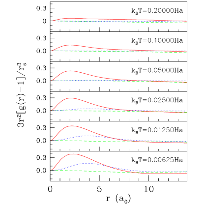
Figure 3: Relative pair density functions for the spin-unpolarized electron-hole system at $r_{s}=10$, showing formation of excitons and biexcitons. Correlation functions $3r^{2}[g(r)-1]/r_{s}^{3}$ are shown for opposite species (solid lines), same species with opposite spin (dotted lines), and same species with same spin (dashed lines). Normalization is chosen so that area under the curve represents the change in density relative to a uniform distribution. At $T=0.05$ Ha the area under the opposite species curve is approximately one, indicating excitons. At $T=0.00625$ Ha the area under the opposite species curve is approximately two, and the area under the same species, opposite spin curve is approximately one, indicating biexcitons.

In Figure 3 we show evidence of exciton and biexciton formation in a system of fourteen spin-unpolarized electron-hole pairs at a density $r_{s}=10$ computed using free particle nodal surfaces. The figure shows the change in the pair correlation functions, normalized so that the area under the curve represents the radial change in density relative to a uniform distribution. Electrons and holes attract each other, and the location of the peak near $r=2a_{0}$ agrees very well with the exciton radius, $a_{x}=2a_{0}$. The area under the curve at $T=0.05$ Ha is approximately one, so we interpret this as an excitonic regime.

Also shown in Figure 3 is the deviation of the pair correlation function from a uniform distribution between particles of the same species. The dotted lines are same species with opposite spin, and the dashed lines are same species with the same spin. Although the relative density for same species with like spin always dips negative, indicating a depletion, particles of the same species with opposite spin have some attraction. At $T=0.00625$ Ha the area under the same species, opposite spin curve is approximately one, while the area under the opposite species curve has increased to two. This means that a particle is likely to have three other particles near it: one particle of the same species with opposite spin, and two particles of the other species (one in each spin state). We interpret this as formation of biexcitons.

To summarize, for a system of spin-unpolarized electron-holes at a density of $r_{s}=10$, we find excitonic formation beginning below $T\approx 0.2$ Ha $=0.8E_{x}$, with an excitonic regime formed by $T\approx 0.05$ Ha $=0.2E_{x}$. Below this temperature, excitons begin to pair together, and by $T\approx 0.00625$ Ha $=0.025E_{x}$ we see biexcitons form.

5.2 Permuting excitons and the superfluid transition

As discussed previously, Bose condensation of excitons is expected to be seen as long cycles of permuting electrons. The excitons should appear as electron and hole paths propagating side by side in imaginary time. One way to look for Bose condensation is to look for such a feature in a graphical representation of the paths.

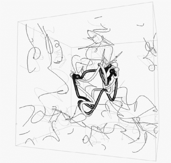
(a)

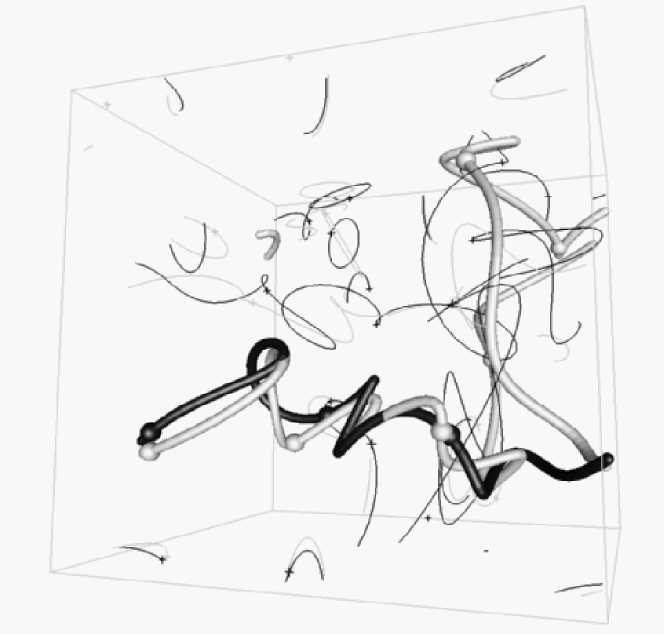
(b)

Figure 4: A “snapshot” taken from a PIMC simulation of 19 spin-polarized electron-hole pairs at $r_{s}=6$ and $T=0.0125$ Ha. To enhance visual clarity, Fourier smoothing has been used to eliminate the imaginary- time high frequency noise. The dark-colored paths represent electrons and the light-colored paths represent holes. The thick paths in the panels show: (a) two permuting excitons, (b) a winding electron-hole pair. The thin paths represent all the other particles in the simulation. Paired nodal surfaces were used for these calculations.

In Figure 4 is a “snapshot” from a simulation of 19 electron-hole pairs, one panel high-lighting a pair of permuting excitons, the other 3 permuting excitons winding around the boundaries. What is interesting in this picture is the complexity of the fermion pairing. Close examination shows that electrons and hole are almost always paired up. However one does not simply have pairing between two like membered exchanges of the same length. Rather there is an intertwined network of coupled electron and hole exchanges. This is reflected in the mass and charged coupled winding statistics.

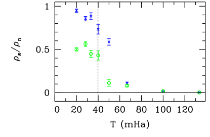
Figure 5: Superfluid density: mass coupled superfluid density, charge-coupled superfluid density, for electrons and holes at $r_{s}=4$.

Shown in Figure 5 are the mean squared winding numbers both for mass and charge. A superfluid is defined as a system that decouples from a boost in the boundaries: the appropriate winding number to compute is to add the windings for the electrons and holes before one squares. This number shows a rapid increase near the peak in the specific heat and rapidly approaches unity. An estimate of $T_{c}$ can be determined by a finite size scaling study of the superfluid density.

The second curve shows the response of the system to a weak imposed magnetic field. A superconductor will exclude magnetic fields: the Meisner effect. A magnetic field couples to the charge, so the appropriate winding number is the electron winding minus the hole winding. For tightly bound excitons, the electron winding would always equal the hole winding, since one has a neutral object which does not response to the applied field. We find a partial response, substantial screening does occur. Further studies need to be made to understand if this curve scales to zero in the thermodynamic limit. In a system of unpolarized particles, one would have additional spin response functions.

Figure 6: Kinetic, potential and total energy, and specific heat for 19 spin-polarized excitons as a function of temperature, at densities $r_{s}=5$ and $r_{s}==6$. Vertical dashed lines are the ideal gas transition temperature for each density. Densities are: $r_{s}=6$ (left) and $r_{s}=5$ (right).

A characteristic feature of Bose condensation is the peak in the specific heat at the superfluid transition. Not only is the feature prominent in both weakly and strongly interacting bosons, even superconducting transitions exhibit a similar peak.

We plot the specific heat as estimated from numerical derivatives of our total energy values in Figure 6. For $r_{s}=6$ we see a clear peak near the transition line, and similar behavior for $r_{s}=5$. For higher density of $r_{s}=4$ the data is much too noisy show any real features but we do see signs of the lambda transition. Since the specific heat is a derivative of the energy, statistical errors in the energy get magnified. The observation of the lambda transition in the specific heat is computationally demanding and not a particularly good indicator of the phase transition.

In Figure 6 we plot the kinetic, potential, and total energies as a function of temperature for densities $r_{s}=6,5$ and 4. For reference, we show the transition temperature $T_{c}^{0}$ for a non-interaction system as a vertical dotted line in each of the figures. We see qualitatively different behavior in the energy above and below $T_{c}^{0}$. The kinetic energy changes slope, from nearly constant below $T_{c}^{0}$ to a slope in the range $2k_{B}$ to $3k_{B}$ above $T_{c}^{0}$. The potential energy becomes slightly less negative below $T_{c}^{0}$. We interpret the different kinetic energy behaviors as changing from a classical thermal distribution of excitonic motion (and internal excitations of the excitons) above $T_{c}^{0}$ to a Bose condensed state with little excess kinetic energy below $T_{c}^{0}$.

The flat behavior of the energy of low temperature is an indication of Bose like (not Fermi) excitation spectra. Once one is below the transition, there are few excitations.

5.3 Energy at low temperature

At low temperature and low density, the interactions between excitons are described by the exciton-exciton scattering length, $a_{s}=3.0a_{0}$, as calculated in Ref. [19]. We have calculated the total energy of 19 spin-polarized electron-hole pairs at $T=0.00625$ Ha and a range of densities, $r_{s}=4,5,6,7,8,9$, and $10$ using paired nodal surfaces. We plot the total energies in Figure 7.

Figure 7: Condensate energy as a function of density for spin-polarized excitons. Solid line is Bogoliubov theory, data points are from PIMC.

The ground state energy of Bose condensed excitons well below the transition temperature is given by Bogoliubov theory for a dilute Bose gas [20],

$$\frac{E}{V}=\frac{2\pi a_{s}}{m}\left(\frac{N}{V}\right)^{2}\left[1+\frac{128}{15\sqrt{\pi}}a_{s}^{3/2}\left(\frac{N}{V}\right)^{1/2}\right]\approx\frac{2.25}{r_{s}^{3}}\left[1+\frac{12.2}{r_{s}^{3/2}}\right].$$ (13)

$N$ is the number of bosons, and $V$ is the volume of the (periodic) box. The last expression is for spin-polarized excitons with a mass $m=2$ and and a scattering length of $a_{s}=1.5a_{x}=3.0a_{0}$, as found in Ref. [19]. This assumes that only two particle collisions are significant, $s$-wave scattering dominates, and only interactions involving the condensate are important. The first two assumptions hold for a low-density system, $N/V\ll a_{s}^{-3}$. The last assumption is valid when the condensate fraction is large, so that the energy contribution due to the interactions between non-condensed particles is negligible.

Simulations with $r_{s}\leq 8$ agree very well with the theory, (note there are no adjustable parameters) as shown in Figure 7. Simulations at lower densities, have higher energies because of thermal effects. The transition temperature decreases with density, taking on the values $T_{c}^{0}=0.07875$ and $T_{c}^{0}=0.06375$ at $r_{s}=9$ and $r_{s}=10$, respectively. Few of the excitons are condensed at these densities, hence the energies are above the Bogoliubov ground state energy. We estimate the energy per pair of non-condensed excitons as the exciton binding energy, plus $3/2k_{B}T$ for the kinetic energy of the excitons, plus twice the Bogoliubov interaction energy (the factor of two arises from the exchange term, which is not present in the condensate) and plot that as a dotted line in the figure. The agreement confirms our interpretation of the data.

References

- [1]
- [2] R. P. Feynman, Phys. Rev. 91, 1291 (1953).
- [3] D. M. Ceperley, Rev. Mod. Phys. 67, 279 (1995).
- [4] D. M. Ceperley, J. Stat. Phys. 63, 1237 (1991).
- [5] L. N. Cooper, Phys. Rev 104, 1189 (1956).
- [6] L. Gilgien, Ph.D. thesis, Université de Genève, 1997.
- [7] D. M. Ceperley, Phys. Rev. Lett. 69, 331 (1992).
- [8] C. Pierleoni, B. Bernu, D. M. Ceperley, and W. R. Magro, Phys. Rev. Lett. 73, 2145 (1994).
- [9] M. D. Jones and D. M. Ceperley, Phys. Rev. Letts 76, 4572 (1996).
- [10] J. Bardeen, L. N. Cooper, and J. R. Schrieffer, Phys. Rev 106, 162 (1957).
- [11] J. Bardeen, L. N. Cooper, and J. R. Schrieffer, Phys. Rev 108, 1175 (1957).
- [12] J. P. Wolfe, J. L. Lin, and D. W. Snoke, in Bose Einstein Condensation, edited by A. Griffin, D. W. Snoke, and S. Stringari (Cambridge, New York, 1995), pp. 281–329. See Ref. [21].
- [13] D. W. Snoke, J. P. Wolfe, and A. Mysyrowicz, Phys. Rev. B 41, 11171 (1990).
- [14] J. L. Lin and J. P. Wolfe, Phys. Rev. Lett. 71, 1222 (1993).
- [15] K. E. O’Hara, Ph.D. thesis, University of Illinois at Urbana-Champaign, 1999.
- [16] M. Randeria, in Bose Einstein Condensation, edited by A. Griffin, D. W. Snoke, and S. Stringari (Cambridge, New York, 1995), pp. 355–392. See Ref. [21].
- [17] A. J. Leggett, in Modern Trends in Condensed Matter Physics, edited by A. Pekalski and J. Przystawa (Springer, Berlin, 1980), pp. 14–27.
- [18] P. D. Grüter, D. M. Ceperley, and F. Laloë, Phys. Rev. Lett. 79, 3549 (1997).
- [19] J. Shumway and D. M. Ceperley, cond-mat/9907309, submitted to Phys. Rev. B (unpublished).
- [20] A. A. Abrikosov, L. P. Gorkov, and I. E. Dzyaloshinski, Methods of Quantum Field Theory in Statistical Physics (Dover, New York, 1963).
- [21] in Bose Einstein Condensation, edited by A. Griffin, D. W. Snoke, and S. Stringari (Cambridge, New York, 1995).