[

Staggered-vorticity correlations in a lightly doped $t$-$J$ model: a variational approach.

Abstract

We report staggered vorticity correlations of current in the d-wave variational wave function for the lightly-doped $t$-$J$ model. Such correlations are explained from the $SU(2)$ symmetry relating $d$-wave and staggered-flux mean-field phases. The correlation functions computed by the variational Monte Carlo method suggest that pairs are formed of holes circulating in opposite directions.

]

Flux phases have been proposed as mean-field solutions to two-dimensional antiferromagnets [3]. For the undoped Heisenberg antiferromagnet, the staggered-flux variational wave function gives a relatively good energy [4, 5, 6], even without the Neel long-range order. However, for doped systems staggered-flux phases would normally break the translational and the time-reversal symmetries, except at the flux value of $\pi$. Besides, the physical meaning of the flux is not transparent. It has been suggested that flux is related to the spin-chirality correlations [7], but such correlations are very complicated for both experimental and theoretical study.

Remarkably, in the case of doped $t$-$J$ or Hubbard models, there is one more indication of a staggered-flux phase. Namely, the current-current correlations may show the staggered-flux pattern inherited from the mean-field phase. We find such a pattern in the Gutzwiller-projected $d$-wave variational wave function for the $t$-$J$ model. Those correlations may be explained by the $SU(2)$ equivalence between the $d$-wave-pairing and staggered-flux phases. Finally, we interpret the staggered-flux structure of current correlations as a pairing between holes of opposite “staggered-vorticity”.

Consider first the $d$-wave variational wave function [4, 5]:

$$\Psi=P_{G}\prod_{k}(u_{k}+v_{k}c^{\dagger}_{k\uparrow}c^{\dagger}_{k\downarrow})|0\rangle,$$ (1)

where $P_{G}$ is the projection onto the states with a fixed number of electrons and without doubly-occupied sites. The coherence factors $u_{k}$ and $v_{k}$ are of the BCS form for $d$-wave pairing:

$$a_{k} \equiv {v_{k}\over u_{k}}={\Delta_{k}\over\xi_{k}+\sqrt{\xi_{k}^{2}+\Delta_{k}^{2}}},$$ (2)

$$\xi_{k} = -2(\cos k_{x}+\cos k_{y})-\mu,$$ (3)

$$\Delta_{k} = \Delta(\cos k_{x}-\cos k_{y}).$$ (4)

For simplicity, we consider the case $\mu=0$. Tuning $\mu$ improves the energy by only 0.2%, and the current correlations reported in this paper remain practically the same.

Using the variational Monte Carlo (VMC) method, we computed the current-current correlations for the wave function (1) in a finite system (2 holes in the $10\times 10$ lattice with periodic-antiperiodic boundary conditions, $\Delta=0.55$). The current on a link $(ij)$ is defined as

$$j_{ij}=-j_{ji}=i(c^{\dagger}_{\alpha i}c_{\alpha j}-c^{\dagger}_{\alpha j}c_{\alpha i}).$$ (5)

The correlation function exhibits a staggered-flux structure (Fig. 1). Since the current vanishes as the hole concentration $x\rightarrow 0$, we have divided the correlation function by $x$. This behavior of the current correlations is observed in the whole range of the gap values $\Delta$. The correlations are smaller at small $\Delta$, which will be interpreted as the limit of staggered flux going to zero. We introduce vorticity $V$ for any plaquet as a sum of the currents around it in the counterclockwise direction: $V=(j_{12}+j_{23}+j_{34}+j_{41})_{\Box}$. The vorticity correlations (Fig. 1b) obtained from the current-current correlations in Fig. 1a have alternating sign with a phase shift of $\pi$, so that the sign of $\langle V(0)V(R)\rangle$ is $(-1)^{R_{x}+R_{y}+1}$.

This staggered-vorticity correlation is a surprising consequence of the projection, because it is absent in the unprojected $d$-wave wavefunction. In order to understand this, we show below that the same wavefunction can be written as a projection of a staggered-flux state. This has the advantage that properties that are obscure in one representation may become obvious in another. For example, the staggered-flux wavefunction is an insulator with gap nodes. The appearance of superconductivity after projection is a surprise, but vorticity and attraction between holes appear naturally, as we shall discuss below.

The basic starting point is the $SU(2)$ symmetry in the fermion representation of the $t$-$J$ model. This is well understood in the undoped case [8], where $SU(2)$ doublets $\psi_{\uparrow i}=(f_{\uparrow i},f_{\downarrow i}^{\dagger})$ and $\psi_{\downarrow i}=(f_{\downarrow i},-f_{\uparrow i}^{\dagger})$ represent the destruction of spin up and spin down in the subspace of one fermion per site. Wen and Lee [9] extended this symmetry away from half filling by introducing a doublet of bosons $b_{i}=(b_{1i},b_{2i})$. The physical electron is represented as an $SU(2)$ singlet formed out of the fermion and boson doublets $c_{\alpha i}=\frac{1}{\sqrt{2}}b_{i}^{\dagger}\psi_{\alpha i}$.

At the level of variational wave functions, the constraint of no double occupation is enforced by projecting the fermion-boson wave function onto the $SU(2)$-singlet subspace of the Hilbert space. On each site, there are only three physical states: spin-up, spin-down and a hole,

$$|\!\uparrow\rangle=f^{\dagger}_{\uparrow}|0\rangle,\;\;\;|\!\downarrow\rangle=f^{\dagger}_{\downarrow}|0\rangle,\;\;\;|\star\rangle={1\over\sqrt{2}}(b^{\dagger}_{1}+b^{\dagger}_{2}f^{\dagger}_{\uparrow}f^{\dagger}_{\downarrow})|0\rangle.$$ (6)

The projector may be written as

$$P_{SU(2)}=\prod_{i}\left(|\!\uparrow\rangle\langle\uparrow\!|+|\!\downarrow\rangle\langle\downarrow\!|+|\star\rangle\langle\star|\right)_{i}.$$ (7)

It should be applied to a mean-field state with the total number of bosons defining the number of doped holes. The mean-field Hamiltonian has the form

$$H= \sum_{\{ij\}}\left[J\psi_{\alpha i}^{\dagger}U_{ij}\psi_{\alpha j}+t(b_{i}^{\dagger}U_{ij}b_{j}+{\rm h.c.})\right]$$ (9)

$$+\sum_{i}a_{i}^{\mu}({1\over 2}\psi_{\alpha i}^{\dagger}\tau_{\mu}\psi_{\alpha i}+b_{i}^{\dagger}\tau_{\mu}b_{i}),$$

where $U_{ij}$ are $SU(2)$ matrices representing generalized hopping amplitudes (mean-field parameters) for nearest-neighbor sites $i$ and $j$.

In the underdoped region, the mean field solution is the staggered-flux phase characterized by

$$U_{ij}=e^{ia_{ij}\tau_{3}},\qquad a^{\mu}_{i}=0.$$ (10)

with $a_{ij}=(-1)^{x(i)+y(j)}\varphi/4$ forming a staggered-flux pattern around plaquets of the lattice, as shown in Fig. 2a (the overall normalization of $U_{ij}$ is of no importance for the wave function). The gauge-invariant variational parameter of the staggered-flux ansatz is the flux per plaquet $\varphi=\sum_{\Box}a_{ij}$. Even though the ground-state wave function breaks time-reversal and translational symmetries, these symmetries are restored after the projection (7).

Even with hole doping, the fermion bands are exactly half-filled, and therefore the number of “no-fermion” sites is equal to the number of “two-fermion” sites. This is shown in Fig.2b. Note that both these sites are spin singlets and have the right spin quantum number for a physical hole. In $SU(2)$ theory, a $b_{1}$ boson is attached to the “no-fermion” site and a $b_{2}$ boson to the “two-fermion” site, and both become physical holes, according to Eq. (6). In the mean field theory, the bosons condense to the bottom of their respective bands, which are located at ${\bf Q}_{1}=0$ and ${\bf Q}_{2}=(\pi,\pi)$. The prescription of constructing an $SU(2)$ projected wavefunction is as follows. The physical wavefunction is specified by the location of the up spins and the holes (circled sites in Fig.2b). A given set of holes is partitioned into all possible “no-fermion” and “two-fermion” sites, denoted by $\{{\bf r}_{1}\}$,$\{{\bf r}_{2}\}$. Each partition specifies a configuration of the staggered flux wavefunction given by a product of two Slater determinants (for spin-up and spin-down spinons). To this we multiply the phase factor $\exp[i\sum_{\{{\bf r}_{1}\},\{{\bf r}_{2}\}}({\bf Q}_{1}\cdot{\bf r}_{1}+{\bf Q}_{2}\cdot{\bf r}_{2})]$ to represent Bose condensation of $b_{1},b_{2}$ and sum over all partitions. An additional sign depending on the ordering of sites is needed to preserve the antisymmetry of the wavefunction. This prescription realizes the projection $P_{SU(2)}$ of a mean-field staggered-flux state to the $SU(2)$ singlet subspace.

FIG. 1.: (a) Current-current correlations for 2 holes in the $10\times 10$ lattice at $\Delta=0.55$ and $\mu=0$. Boundary conditions are periodic in one and antiperiodic in the other direction (the data are averaged over the two orientations). The number on a link is the correlation of the current on this link and of the current on the circled link divided by hole density. The arrows point in the direction of the positive correlations of the current. (b) The same data in the form of vorticity correlations. The number on a plaquet is the vorticity correlation divided by $x$ with the crossed plaquet. (c) Same as (b) for 10 holes in $10\times 10$ lattice.

Next we prove the equivalence of the $SU(2)$ projected staggered flux phase with the pairing state (1). Such an equivalence is known in the undoped case [3], we extend it to doped systems. We note that the mean-field ground state of the staggered flux phase has the form $|\Phi_{mean}\rangle=|\Phi_{f}\rangle\otimes|\Phi_{b}\rangle$, where $|\Phi_{b}\rangle=e^{\bar{b}_{1}B_{1}^{\dagger}+\bar{b}_{2}B_{2}^{\dagger}}|0\rangle$ with $(B_{1},B_{2})=(\sum_{i}b_{1i},\sum_{i}(-1)^{i}b_{2i})$, and $|\Phi_{f}\rangle$ is the fermion state in the staggered flux phase Eqs. (9),(10). Complex numbers $\bar{b}_{1}$ and $\bar{b}_{2}$ parametrize the Bose condensate where $b_{1,2}$ condense into their band bottoms: $B_{a}|\Phi_{b}\rangle=\bar{b}_{a}|\Phi_{b}\rangle$. The $SU(2)$ projection selects the subspace with equal numbers of $B_{1}$ and $B_{2}$ bosons, and therefore states corresponding to different choices of $\bar{b}_{1}$ and $\bar{b}_{2}$ differ after projection only by a one-parameter transformation $\exp(\lambda N_{h})$, where $\lambda$ is a complex parameter, $N_{h}$ is the number of holes. If we fix the average hole concentration, the wave function is defined unambiguously, up to an unimportant gauge $\exp(\lambda N_{h})$ with ${\rm Re}\lambda=0$.

FIG. 2.: (a) Staggered-flux phase. Links with arrows correspond to $a_{ij}=\varphi/4$ in the direction of the arrow. (b) A typical configuration of the half-filled fermion state. Arrows denote fermions. Circled sites are physical holes which are spin singlets made up of either empty or two-fermion sites. $b_{1}$ and $b_{2}$ bosons are assigned to these respective sites.

The staggered-flux mean-field state is related to the $d$-wave state by a $SU(2)$ rotation $W_{i}=\exp[(-1)^{i}{\pi\over 4}\tau_{1}]$:

$$U^{\prime}_{ij}=W_{i}U_{ij}W_{j}^{\dagger}\propto\pmatrix{1&\pm\Delta/2\cr\pm\Delta/2&-1}$$ (11)

where the sign of $\Delta$ is opposite for vertical and horisontal links, and $\Delta$ related to $\varphi$ by

$$\tan{\varphi\over 4}={\Delta\over 2}.$$ (12)

After the $SU(2)$ rotation, the mean field state has the same form, except $|\Phi_{f}\rangle$ is replaced by $|\Phi_{f}^{\prime}\rangle$, the fermion $d$-wave state of the BCS form (1), and the bosonic parameters $\bar{b}_{a}$ are rotated: $\bar{b}_{1}^{\prime}=(\bar{b}_{1}+i\bar{b}_{2})/\sqrt{2}$, $\bar{b}_{2}^{\prime}=(i\bar{b}_{1}+\bar{b}_{2})/\sqrt{2}$. Since the two mean-field states are related by a $SU(2)$ gauge transformation, they lead to the same physical state after the $SU(2)$ projection: $P_{SU(2)}|\Phi_{mean}\rangle=P_{SU(2)}|\Phi_{mean}^{\prime}\rangle$. The freedom in the choice of the bosonic parameters $\bar{b}_{1}$ and $\bar{b}_{2}$ established in the staggered-flux gauge allows us to set $\bar{b}_{2}^{\prime}=0$, then the $SU(2)$ projection becomes equivalent to the conventional Gutzwiller projection. This proves that the $SU(2)$ wave function is identical to the conventionally-projected wave function. Of course, the above proof equally applies to the systems with fixed numbers of holes which we use in our VMC calculation. In this case, the $SU(2)$ projected wave function is identical to that given by Eq. (1).

Note that in the proof of the equivalence of the two wave functions we use $a^{\mu}_{i}=0$ (and, therefore, $\mu=0$ ). A finite $\mu$ in the pairing gauge corresponds to a nonzero value of the Lagrange multiplier $a^{3}_{i}$ (chemical potential). In the staggered-flux gauge, this translates into an on-site pairing term

$$\Delta(\theta_{i})=\mu(e^{i\theta_{i}}f^{\dagger}_{\uparrow i}f^{\dagger}_{\downarrow i}+e^{-i\theta_{i}}f_{\downarrow i}f_{\uparrow i})$$ (13)

with some site-dependent phases $\theta_{i}$. This term only slightly affects the properties of the projected wave function, and we neglect it in the further discussion.

In the ground state of the staggered-flux mean-field Hamiltonian [eq.(9) with $U_{ij}$ given by (10)], the $b_{1}$ and $b_{2}$ bosons attract each other. This can be understood from the correlation function for the “excess density of fermions”:

$$\langle\left(1-n_{f}(i)\right)\left(1-n_{f}(j)\right)\rangle = \langle\left(1-f^{\dagger}_{\alpha i}f_{\alpha i}\right)\left(1-f^{\dagger}_{\beta j}f_{\beta j}\right)\rangle$$ (14)

$$= -\big{|}\langle f^{\dagger}_{\alpha i}f_{\alpha j}\rangle\big{|}^{2}<0$$ (15)

at the mean-field level. This means that around a “no-fermion” hole ($b_{1}$ hole) with $1-n_{f}(i)>0$ there is a region of an increased probability to find a “two-fermion” hole ($b_{2}$ hole) with $1-n_{f}(j)<0$, and vice versa. The mean-field Green’s function $G(i,j)=\langle f^{\dagger}_{\alpha i}f_{\alpha j}\rangle$ decays as $R^{-2}$ at large distances $R=|i-j|$. This is a consequence of the nodes $k=(\pm\pi/2,\pm\pi/2)$ in the mean-field spectrum

$$E(k)\propto\sqrt{\cos^{2}k_{x}+\cos^{2}k_{y}+2\cos{\varphi\over 2}\cos k_{x}\cos k_{y}}.$$ (16)

Thus at the mean-field level, the attraction of the two species of holes leads to a $R^{-4}$ decay of the density-density correlations. After the projection, the attraction becomes much weaker, but still survives, as we shall see from our VMC computations. This attraction between holes was observed earlier [4], but was difficult to explain in the $d$-wave gauge.

In Fig. 3 we plot the correlations of the hole density $n_{h}(i)=1-c^{\dagger}_{\alpha i}c_{\alpha i}$ and of the vorticity $V$ at $\Delta=0.55$ for two holes in a $18\times 18$ lattice as functions of distance. We observe power-law decay of both correlations, $\langle n_{h}(0)n_{h}(R)\rangle\propto\langle V(0)V(R)\rangle\propto R^{-\alpha}$, with the equal exponents $\alpha\approx 1.2$.

The reduction of the exponent $\alpha$ from its mean-field value $\alpha=4$ is due to the projection. For the case of two holes (“zero-doping limit”), this reduction is so strong that $\alpha<2$ and, as a consequence of the sum rule $\sum_{R}\langle n_{h}(0)n_{h}(R)\rangle=n_{h}$ , the two holes become unbound as the size of the system increases.

The proportionalty of the vorticity and density correlations, together with the sign of the vorticity correlations, suggests that the two holes may be thought of as carrying opposite staggered vorticity. This can be justified if we fix the gauge and describe the wavefunction as the staggered-flux phase. At the mean-field level, this breaks the time-reversal symmetry, and the fermions in the filled single-particle states carry a non-zero staggered-vorticity with $\langle j^{f}_{ij}\rangle\neq 0$, where $j^{f}_{ij}=i(f^{\dagger}_{\alpha i}f_{\alpha j}-f^{\dagger}_{\alpha j}f_{\alpha i})$ is the (unphysical) fermion current. The $SU(2)$ projection (7) restores the time-reversal symmetry, and for the projected wave function $\langle j_{ij}\rangle=0$, for the physical current $j_{ij}$. In the staggered-flux gauge (10), at the mean-field level, $j_{ij}\sim j^{f}_{ij}$ for $b_{1}$ holes and $j_{ij}\sim-j^{f}_{ij}$ for $b_{2}$ holes. Thus $\langle j_{ij}\rangle=0$ for the physical current is a result of the balance between the opposite staggered-vorticity of $b_{1}$ and $b_{2}$ holes. The attraction between the two $SU(2)$ species of holes then implies attraction between holes circulating in the opposite directions. For a finite system with two holes, the holes are always of opposite $SU(2)$ types, which resultins in the proportionality between the vorticity and density correlations.

The above picture can be summarized in the expression $\tilde{V}\propto\rho_{1}-\rho_{2}$, where $\tilde{V}$ is the staggered-vorticity $(-)^{R}V(R)$ for the physical current $j_{ij}$, and $\rho_{1,2}$ are the densities of the two bosons $b_{1,2}$. The correlations of the staggered-vorticity and of $\rho_{1}-\rho_{2}$ are related $\langle\tilde{V}(R)\tilde{V}(0)\rangle\propto\langle\rho_{1}(R)\rho_{1}(0)\rangle+\langle\rho_{2}(R)\rho_{2}(0)\rangle-2\langle\rho_{1}(R)\rho_{2}(0)\rangle$. When there are only two holes $\langle\rho_{1}(R)\rho_{1}(0)\rangle=\langle\rho_{2}(R)\rho_{2}(0)\rangle=0$, we find that

$$\langle\tilde{V}(R)\tilde{V}(0)\rangle\propto-\langle\rho(R)\rho(0)\rangle$$ (17)

where $\rho=\rho_{1}+\rho_{2}$ is the total density of the holes. The minus sign explains the $\pi$ phase shift seen in Fig. 1.

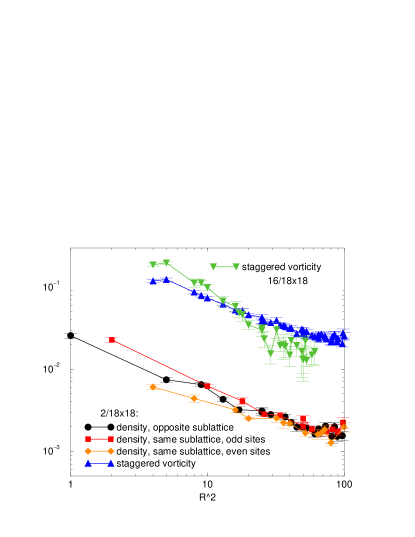
FIG. 3.: Hole density and staggered-vorticity correlations for 2 holes and staggered-vorticity correlations for 16 holes in the $18\times 18$ lattice. Boundary conditions are periodic in one and antiperiodic in the other direction, $\Delta=0.55$. The correlation functions are divided by the density of holes $x$ and plotted as a function of the squared distance. The data are obtained as a result of averaging over $2\cdot 10^{4}$ samples for $2/18\times 18$ system and $2\cdot 10^{3}$ samples for $16/18\times 18$ system.

If we assume pairing between holes of opposite staggered vorticity, we may interpret the vorticity correlations as the hole correlations within one pair which allow us to determine the strength of the pairing correlation (even for finite density of holes) and measure the size of pairs. At finite density of holes, the correlation of the staggered-vorticity decay faster. In Fig. 4b we present the correlation for 16 holes in $18\times 18$ lattice (nearly 5% doping) at $\Delta=0.55$. We find $\alpha\approx 2.2$. The increase of $\alpha$ above $2$ may be interpreted as a formation of bound hole pairs (and hence the onset of superconductivity). The small value of $\alpha-2$ after the projection implies that the pairs are bound very loosely and their size is large. In this case, the nearest-neighbor pairing amplitude $\langle c_{i\uparrow}c_{j\downarrow}\rangle$ is small, which may account for numerical conclusions about the absence of superconductivity at $J/t<0.5$ [10, 11].

While the staggered vorticity correlation is found for a superconducting wavefunction, we speculate that the phase coherence of the bosons may not be crucial and that such correlation may survive above T_c in the pseudogap state, and indeed serves as a signature of that state. Unfortunately, detection of this correlation may be difficult. We estimate that the fluctuating current generates a fluctuating staggered magnetic field of order 40 G. This field will contribute to the relaxation of the $Y$ nuclei, which are ideally sited above the center of the plaquets. However, we do not have dynamical information at present and it is difficult to predict the magnitude of this orbital relaxation. Another possibility is to freeze in some staggered field pattern around an impurity site. If some $Y$ is replaced by an impurity with spin ${\bf S}$ which strongly couples to the Cu-O plane, we may use a magnetic field to align the spin and therefore create a static orbital current via the ${\bf L}\cdot{\bf S}$ term. This local orbital current may then generate a static staggered pattern around it, which may be detected by shifts in the $Y$ NMR line. Perhaps a more promising way to test our prediction is to look for this effect in exact diagonalization of small systems.

We thank H. Alloul for helpful discussions and we acknowledge the support by NSF under the MRSEC program DMR98-08941.

REFERENCES

- [1]
- [2] Present address: Institut für Theoretische Physik, ETH-Hönggerberg, CH-8093 Zürich, Switzerland.
- [3] For a review, see F. C. Zhang, C. Gros, T. M. Rice, and H. Shiba, Supercond. Sci. Technol. 1 (1988), 36.
- [4] C. Gros, Ann. Phys. 189 (1989), 53.
- [5] H. Yokoyama and M. Ogata, J. Phys. Soc. Jpn. 65 (1996), 3615.
- [6] D. V. Dmitriev, V. Ya. Krivnov, V. N. Likhachev, and A. A. Ovchinnikov, Fiz. Tv. Tela. 38 (1996), 397. [Soviet Physics Solid State Physics]
- [7] P. A. Lee and N. Nagaosa, Phys. Rev. B 46 (1992), 5621.
- [8] I. Affleck et al., Phys. Rev. B 38 (1988), 745.
- [9] X.-G. Wen and P. A. Lee, Phys. Rev. Lett. 76 (1996), 503.
- [10] C. T. Shih, Y. C Chen, H. Q. Lin, and T. K. Lee, Phys. Rev. Lett. 81 (1998), 1294.
- [11] E. S. Heeb and T. M. Rice, Europhys. Lett. 27 (1994), 673.