Dynamical TAP approach to mean field glassy systems

Abstract

The Thouless, Anderson, Palmer (TAP) approach to thermodynamics of mean field spin-glasses is generalised to dynamics. A method to compute the dynamical TAP equations is developed and applied to the p-spin spherical model. In this context we show to what extent the dynamics can be represented as an evolution in the free energy landscape. In particular the relationship between the long-time dynamics and the local properties of the free energy landscape shows up explicitly within this approach. Conversely, by an instantaneous normal modes analysis we show that the local properties of the energy landscape seen by the system during its dynamical evolution do not change qualitatively at the dynamical transition.

If at large times a system relaxes toward the equilibrium state, its dynamics is called “equilibrium dynamics” and equilibrium properties as the fluctuation dissipation relation and the time translation invariance hold. In this case the departures of the dynamical probability measure from the Gibbs measure vanish at large times, therefore the relationships between thermodynamics and long-time dynamics are obvious.
However there are many physical cases, in which a system remains far from equilibrium also at long times. In the following we focus on glassy systems, for which relaxation times become so long at low temperature that these systems are not in equilibrium on laboratory time scales [1]. In this case it is important to understand to what extent pure static concepts (e.g. the free energy landscape) can be related to the long-time dynamics.
For thermodynamics the relevant landscape is the free energy one. Different authors [2] proposed that this landscape is relevant also for dynamics and can be considered, at least at the simplest level, as the landscape on which the dynamical evolution takes place. For example for a spin system the landscape for dynamics would be the free energy as a function of local magnetisations $m_{i}(t)$ and the dynamical variable would be the set of the averaged (over different thermal histories) local magnetisations . At the simplest level the dynamical evolution would be a superposition of two phenomena: a gradient descent in this free energy landscape and jumps between different states with a probability given by a generalised Arrhenius law: $\exp(-\beta\Delta F)$, where $\Delta F$ is the free energy barrier between two states.
However this is far from obvious and up to now a proof of these claims is not available. The main difficulty is that in general the free energy landscape is not known and the long-time dynamics is not solved.
This “Landscape Paradigm” [2] has received a firm theoretical basis in the case of mean field frustrated systems, for which an analytic solution of the thermodynamics [3] and of the asymptotic out of equilibrium regime [1] is in general available.
For these models it was shown that a complicated energy function can lead to a rugged free energy landscape and to an infinite number of correlated states. Thouless, Anderson and Palmer (TAP) [4] computed for the Sherrington Kirkpatrick model [5] the free energy as a function of local magnetisations. At low temperature the TAP free energy has an infinite number of minima; each one corresponds to a different possible state. It has been shown that their weighted sum (with the Boltzmann weight) gives back equilibrium results[6]. Moreover states are correlated and organised in a ultra-metric structure. This is encoded in the Parisi’s solution [8] and was explicitly shown in the cavity approach [7] developed by Mézard, Parisi and Virasoro, which is a way to solve the minimisation equations of the TAP free energy.
Furthermore at low temperature these systems remain out of equilibrium also at very large times [1] and their long-time dynamical behaviour exhibits non trivial features like violation of the fluctuation-dissipation theorem and ageing [9].
In particular for the p-spin spherical model Cugliandolo and Kurchan [9] showed that, even if the system remains always out of equilibrium, the long-time dynamical behaviour can be interpreted in terms of some properties of the free energy landscape. The most intriguing fact is that the properties of the free energy landscape relevant for long time dynamics and thermodynamics are completely different. These results indicate that, at least in this mean field case, there is a close relationship between long-time dynamics and the free energy landscape, which therefore has a meaning on its own also in an out of equilibrium regime. Besides, we note that a connection between the free energy landscape and the long-time out of equilibrium dynamics is very interesting not only for its theoretical implications, but also from a technical point of view. In fact this relationship allows to obtain results about dynamics by a pure static computation [10, 11].
However, the reason of this relationship is not clear. Is the description of the dynamics as an evolution on the free energy landscape correct or does something else happens, but always such that the relationship found in [9] between the asymptotic behaviour and the free energy landscape is satisfied ?
Up to now an answer to this question has been given only for the zero temperature Langevin dynamics of p-spin ($p\geq 2$) spherical models [12]. In this case there is no thermal disorder, so it is clear that a landscape over which the dynamics takes place exists and is the energy landscape (or the free energy one, because at zero temperature they coincide). In [12] it was shown that at least at zero temperature the main reason of ageing is the flatness of the landscape seen during the long-time dynamics .
The regularity of the dynamical equations near $T=0$ and the interpretation of the asymptotic behaviour in terms of TAP free energy [9] seem to indicate that the above scenario might be true also at non zero temperature. However, in this description of ageing it is implicitly assumed that at large times a landscape for dynamics should exist and that this landscape should be related to TAP free energy. Thus, the question about the relationship among dynamical behaviour and free energy landscape arises again.

In this article we clarify this relationship for the p-spin spherical model. The thermodynamical and the dynamical behaviours of this model exhibit strong analogies with the phenomenology of super-cooled liquids, the glass transition and the glassy phase [13, 1, 14]. Moreover the dynamical theory of the p-spin spherical model has a close relationship [15] with the Mode Coupling theory [16], which serves as a basis for some theories of super-cooled liquids. For these reasons many authors consider that the p-spin spherical model provides a mean field description of the glass transition and of the glassy phase.

For this model the TAP free energy was computed and studied in detail [17, 18] and an analytic solution of the asymptotic out of equilibrium regime is available [9, 19]. To understand the reasons of the connection found in [9] between TAP free energy and the asymptotic behaviour, we will compute the equations satisfied by the local magnetisations $m_{i}(t)=\left<s_{i}(t)\right>$ (where $\left<\cdot\right>$ means the average over the thermal noises) without performing the average over disorder. This is the generalisation to dynamics of the Thouless, Anderson and Palmer approach [4].
We will show that the dynamical evolution of the local magnetisations corresponds to a relaxation in the free energy landscape (in a sense which we will precise) only for very large times and for particular initial conditions; in all the other cases the dynamics is characterised by a memory term, which makes the evolution non-Markovian. Moreover the study of the dynamical TAP equations shows that the stationary points of the static free energy and the free energy Hessian in these points are closely related to the long-time dynamical behaviour, as was already found from the solution of the equations on the correlation and the response functions in [9, 11, 20]. Our results explicitly show that the scenario for slow dynamics found in [12] remains valid also at finite temperature: ageing is due to the motion in the flat directions of the free energy landscape in presence of a vanishing source of drift.
Finally we show that already for the simple case of the p-spin spherical model an analysis of the local properties of the energy landscape is not adequate to identify the dynamical glass transition. We will compute the spectrum of the energy Hessian for dynamical configurations seen during the dynamical evolution. The eigenvectors of the energy Hessian are called instantaneous normal modes in liquid theory and have been introduced to represent the short-time dynamics of liquids within a harmonic description [21].
We will show that the local properties of the energy landscape seen during the dynamical evolution do not change qualitatively at the dynamical glass transition but at a higher temperature $T_{0}$, which seems to be related to the damage spreading transition [22]. This indicates that at the dynamical glass transition the energy landscape seen by the system remains locally the same, whereas its global properties change and this can be observed by analysing the local properties of the free energy landscape.

The paper is organised as follows: in section I we derive the static TAP free energy for mean field spin glass models. This section serves as an introduction to the method applied in the following to derive the dynamical TAP free energy. In section II this method is applied to derive the dynamical TAP equations via the analogy between the dynamical theory and a supersymmetric static theory. In section III the asymptotic analysis of the dynamical TAP equations is performed. In section IV the local properties of the energy landscape seen during the dynamical evolution is analysed. Finally we conclude in section V.

I Static TAP approach

A useful function in the study of phase transitions is the Legendre transform of free energy. This function, which can be interpreted as the effective potential whose minima represent different possible states, gives an intuitive (and quantitative) description of phase transitions. Consider for example ferromagnetic systems. In this case the effective potential is a function of magnetisation. The ferromagnetic transition corresponds to the splitting of the paramagnetic minimum in the two ferromagnetic minima. A vanishing external magnetic field breaks the up-down symmetry and fixes the system in one of the two possible ferromagnetic states.
Generally, frustrated systems are characterised by a complicated energy landscape, which can give rise eventually to the existence of many possible states. In this case it is not possible to characterise the states a priori studying the various possible schemes of spontaneous symmetry breaking. Thus, the effective potential has to be computed as a function of the averaged microscopic configuration and this is what Thouless, Anderson and Palmer did for the Sherrington-Kirkpatrick model. They derived the Legendre transform of the free energy with respect to the local magnetic fields $h_{i}$, obtaining the effective potential (called now TAP free energy) which is a function of the local magnetisations $m_{i}$ for a fixed (but typical) disorder configuration. At low temperature the TAP free energy has an infinite number of minima; each one corresponds to a different possible state. It has been shown that their weighted sum (with the Boltzmann weight) gives back equilibrium results[6] found by the replica [8] or the cavity method[3].

In this section we show how the static TAP free energy can be derived for mean field spin glass models. In this way we present in a simple case the strategy which we will follow to compute dynamical TAP equations. The derivations of the static TAP equations presented in the literature [23, 18] seem to be quite often model dependent and rather involved. Therefore we hope that this section may be also useful to show an easy way to obtain the TAP free energy for a generic mean field model. It does not matter if one considers spherical or Ising spins, two body or many body interactions.

A straightforward way to compute the TAP free energy for mean field (completely connected) spin glass models consists in finding a good perturbative expansion such that using the properties of typical disorder configurations it is possible to show that only a finite number of terms of the perturbation series does not vanish.
Following this strategy we will compute the Legendre transform of the free energy with respect to $\left<S_{i}\right>$ and $\sum_{i=1}^{N}\left<S_{i}^{2}\right>$. One may wonder why we Legendre transform also with respect to $\sum_{i=1}^{N}\left<S_{i}^{2}\right>$; the reason is that otherwise the perturbation expansion would contain an infinite number of terms.
Note that for Ising spins the average $\sum_{i=1}^{N}\left<S_{i}^{2}\right>$ is trivial, so we will Legendre transform only with respect to magnetisations. This is a peculiarity of the Ising spins, which disappears for spherical (or Potts) spins and in the dynamical case.

A Static TAP equations

We are finally in position to define the TAP free energy $\Gamma(\beta,m_{i},l)$ which depends on the magnetisation $m_{i}$ at every site $i$ and on the spherical parameter $l$ (for Ising spins $l$ is absent). $\Gamma$ is the Legendre transform of the “true” free energy:

$$-\beta\Gamma(\beta,m_{i},l)=\ln\mbox{Tr}_{\{S_{i}\}}\exp\left(-\beta H(\{S_{i}\})-\sum_{i}h_{i}(S_{i}-m_{i})-\frac{\lambda}{2}\sum_{i=1}^{N}(S_{i}^{2}-l)\right)\quad.$$ (1)

For Ising spins $\mbox{Tr}_{\{S_{i}\}}=\sum_{\{S_{i}\}}$ and for spherical spins $\mbox{Tr}_{\{S_{i}\}}=\int_{-\infty}^{+\infty}\prod_{i=1}^{N}dS_{i}$. The Lagrange multipliers $h_{i}(\beta)$ fix the magnetisation at each site $i$: $\left<S_{i}\right>=m_{i}$ and $\lambda(\beta)$, which is present only for spherical models, enforces the condition $\sum_{i=1}^{N}\left<S_{i}^{2}-l\right>=0$. $\left<\cdot\right>$ denotes the thermal average and $N$ is the number of spins.
Once $\Gamma$ is known, the equation $-\frac{2}{N}\frac{\partial\beta\Gamma}{\partial l}{\Big{|}}_{l=1}=\lambda$ fixes the spherical constraint ($\sum_{i}S_{i}^{2}=N$) and gives the spherical multiplier as a function of $m_{i}$, whereas $-\frac{\partial\beta\Gamma}{\partial m_{i}}{\Big{|}}_{l=1}=h_{i}$ are the TAP equations, which fix the values of local magnetisations.
In the following we focus on the p-spin Hamiltonian:

$$H(\{S_{i}\})=-\sum_{1\leq i_{1}<\cdots<i_{p}\leq N}J_{i_{1},\cdots,i_{p}}S_{i_{1}}\cdots S_{i_{p}}\quad,$$ (2)

where the couplings are Gaussian variables with zero mean and average $\overline{J_{i_{1},\cdots,i_{p}}^{2}}=\frac{p!}{2N^{p-1}}$.

The standard perturbation expansion for the generalised potential $\Gamma$ is rather involved [24, 18] and cannot be directly applied to the Ising case. Thus, we prefer to follow the approach developed for the Sherrington-Kirkpatrick model by T. Plefka [25] and A. Georges and S. Yedidia [26] because is simple and can be directly applied to all mean field spin glass models.
They obtained the TAP free energy for the Sherrington-Kirkpatrick model expanding $-\beta\Gamma$ in powers of $\beta$ around $\beta=0$:

$$-\beta\Gamma(\beta,m_{i},l)=\sum_{n=0}^{+\infty}-\frac{\partial^{n}(\beta\Gamma)}{\partial\beta^{n}}{\Bigg{|}}_{\beta=0}\frac{\beta^{n}}{n!}\quad.$$ (3)

For a general system this corresponds to a $\frac{1}{d}$ expansion ($d$ being the spatial dimension) around mean field theory [26]; so it is not surprising that for mean field spin glass models only a finite number of terms survives. The zeroth- and first-order terms give the “naïve” TAP free energy, whereas the second term is the Onsager reaction term.

From the definition of $-\beta\Gamma$ given in equation (1), we find for Ising spins:

$$-\beta\Gamma_{I}(\beta,m_{i}){\Bigg{|}}_{\beta=0}=-\sum_{i}^{N}\left[\frac{1+m_{i}}{2}\ln\left(\frac{1+m_{i}}{2}\right)+\frac{1-m_{i}}{2}\ln\left(\frac{1-m_{i}}{2}\right)\right]$$ (4)

and for spherical spins:

$$-\beta\Gamma_{S}(\beta,m_{i},l){\Bigg{|}}_{\beta=0}=\frac{N}{2}\ln\left(l-\frac{1}{N}\sum_{i=1}^{N}m_{i}^{2}\right)\quad.$$ (5)

These are the entropies of non interacting Ising or spherical spins constrained to have magnetisation $m_{i}$.
The linear term in the power expansion (3) of the TAP free energy equals:

$$-\beta\frac{\partial(\beta\Gamma_{S,I})}{\partial\beta}{\Bigg{|}}_{\beta=0} = \beta\sum_{1\leq i_{1}<\cdots<i_{p}\leq N}J_{i_{1},\cdots,i_{p}}\left<S_{i_{1}}\cdots S_{i_{p}}\right>_{\beta=0}-$$ (7)

$$-\beta\sum_{i}^{N}\frac{\partial h_{i}}{\partial\beta}{\Bigg{|}}_{\beta=0}\left<S_{i}-m_{i}\right>_{\beta=0}-\beta\frac{\partial\lambda}{\partial\beta}{\Bigg{|}}_{\beta=0}\sum_{i=1}^{N}\left<S_{i}^{2}-l\right>_{\beta=0}\quad,$$

where the last sum is present only for spherical models. The second and the third term are zero because of Lagrange conditions; moreover at $\beta=0$ the spins are decoupled so all the thermal averages are trivial:

$$-\beta\frac{\partial(\beta\Gamma_{S,I})}{\partial\beta}{\Bigg{|}}_{\beta=0}=\beta\sum_{1\leq i_{1}<\cdots<i_{p}\leq N}J_{i_{1},\cdots,i_{p}}m_{i_{1}}\cdots m_{i_{p}}\quad.$$ (8)

This “mean field” energy together with the zeroth-order term gives the standard mean field theory, which becomes exact for infinite-ranged ferromagnetic system. The Onsager reaction term comes from the quadratic term in the expansion (3):

$$-\frac{\beta^{2}}{2}\frac{\partial^{2}(\beta\Gamma_{S,I})}{\partial\beta^{2}}{\Bigg{|}}_{\beta=0} = \frac{\beta^{2}}{2}\left<\left(\sum_{1\leq i_{1}<\cdots<i_{p}\leq N}Y_{i_{1},\cdots,i_{p}}\right)^{2}\right>^{c}_{\beta=0}\quad,$$ (9)

$$Y_{i_{1},\cdots,i_{p}} = J_{i_{1},\cdots,i_{p}}S_{i_{1}}\cdots S_{i_{p}}-(S_{i_{1}}-m_{i_{1}})m_{i_{2}}\cdots m_{i_{p}}-$$ (12)

$$\cdots-m_{i_{1}}\cdots m_{i_{p-1}}(S_{i_{p}}-m_{i_{p}})\quad.$$

To compute this term we have used the following Maxwell relations:

$$\frac{\partial h_{i}}{\partial\beta}{\Bigg{|}}_{\beta=0} = -\frac{\partial}{\partial m_{i}}\frac{\partial(\beta\Gamma_{S,I})}{\partial\beta}{\Bigg{|}}_{\beta=0}$$ (13)

$$\frac{\partial\lambda}{\partial\beta}{\Bigg{|}}_{\beta=0} = -\frac{2}{N}\frac{\partial}{\partial l}\frac{\partial(\beta\Gamma_{S})}{\partial\beta}{\Bigg{|}}_{\beta=0}$$ (14)

Using the statistical properties of the couplings it is easy to check that the only terms giving a contribution of the order of $N$ correspond to the squares of $J_{i_{1},\cdots,i_{p}}$:

$$-\frac{\beta^{2}}{2}\frac{\partial^{2}(\beta\Gamma_{S,I})}{\partial\beta^{2}}{\Bigg{|}}_{\beta=0} = \frac{\beta^{2}}{2}\sum_{1\leq i_{1}<\cdots<i_{p}\leq N}\left<Y^{2}_{i_{1},\cdots,i_{p}}\right>^{c}_{\beta=0}$$ (15)

$$= \frac{\beta^{2}}{2p!}\sum_{i_{1}\neq\cdots\neq i_{p}}J^{2}_{i_{1},\cdots,i_{p}}{\Big{(}}\left<S^{2}_{i_{1}}\right>_{\beta=0}\cdots\left<S^{2}_{i_{p}}\right>_{\beta=0}-m^{2}_{i_{1}}\cdots m^{2}_{i_{p}}$$ (17)

$$-p\left<(S_{i_{1}}-m_{i_{1}})^{2}\right>_{\beta=0}m^{2}_{i_{2}}\cdots m^{2}_{i_{p}}{\Big{)}}\quad.$$

Using again the statistical properties of the couplings and neglecting terms giving a contribution of an order smaller than $N$ we find that the reaction term depends on $m_{i}$ through the overlap $q=\frac{1}{N}\sum_{i}m_{i}^{2}$ only:

$$-\frac{\beta^{2}}{4}\frac{\partial^{2}(\beta\Gamma_{I})}{\partial\beta^{2}}{\Bigg{|}}_{\beta=0} = \frac{\beta^{2}N}{2}\left(1-q^{p}-p(q^{p-1}-q^{p})\right)\quad,$$ (18)

$$-\frac{\beta^{2}}{2}\frac{\partial^{2}(\beta\Gamma_{S})}{\partial\beta^{2}}{\Bigg{|}}_{\beta=0} = \frac{\beta^{2}N}{4}\left(l^{p}-q^{p}-p(lq^{p-1}-q^{p})\right)\quad.$$ (20)

Higher derivatives in equation (3) lead to terms which can be neglected because they are not of order of N [18, 26]; so collecting (4),(5),(8),(18) and (20) we find the TAP free energy for Ising and spherical p-spin models. Deriving the free energy with respect to magnetisations $m_{i}$ and the spherical parameter $l$ (in the spherical case) one finds the TAP equations. For instance for spherical spins we find:

$$\frac{m_{i}}{1-q}=\frac{\beta}{(p-1)!}\sum_{i_{2}\neq\cdots\neq i_{p}(\neq i)}J_{i,i_{2},\cdots,i_{p}}m_{i_{2}}\cdots m_{i_{p}}-\frac{\beta^{2}}{2}p(p-1)q^{p-2}(1-q)m_{i}\quad,$$ (21)

$$\lambda=\frac{1}{1-q}+\frac{p\beta^{2}}{2}(1-q^{p-1})\quad.$$ (22)

These equations admit for certain temperatures an infinite number of solutions. This is a fundamental characteristic and difficulty of mean field spin glasses.

It has been shown that the weighted sum of the local minima of the TAP free energy gives back equilibrium results found by the replica or the cavity method [6, 18]:

$$Z=\sum_{\alpha}e^{-N\beta f_{\alpha}}\qquad,$$ (23)

where $f_{\alpha}$ is the TAP free energy of a stable solution $\{m_{i}^{\alpha}\}$ of TAP equations. The different TAP states can be grouped with respect to their free energy; then the partition function can be rewritten as:

$$Z=\int dfe^{-N(\beta f-\Sigma(f;\beta))}\qquad$$ (24)

where $N\Sigma(f;\beta)$ is the logarithm of the number of TAP states with free energy $f$ and is called complexity [27, 13, 18].
Note that states which do not have the minimum free energy can dominate the sum in (24) if their number is very large.

Finally, we note that it was crucial to Legendre transform also with respect to $\frac{1}{N}\sum_{i=1}^{N}S_{i}^{2}$, otherwise in (3) the derivatives higher than the second order would not vanish and an infinite number of terms should be re-summed. This re-summation is automatically achieved if one Legendre transform also with respect to $\frac{1}{N}\sum_{i=1}^{N}S_{i}^{2}$.

B A brief survey on the p-spin spherical model

In the following we recall very briefly some results on the thermodynamics and the dynamics of the p-spin spherical model which will be useful for the asymptotic analysis of the dynamical TAP equations. A detailed review has been done by Barrat [28].

1 The thermodynamics

The thermodynamics of the p-spin spherical model has been studied within the replica approach in [29], whereas the TAP equations have been analysed in [17, 18].
It has been shown that there is a high temperature regime $T>T_{d}$, $T_{d}=\sqrt{\frac{p(p-2)^{p-1}}{2(p-1)^{p-1}}}$, for which the paramagnetic state $m_{i}=0$ dominates the partition function, i.e. $Z=e^{-N\beta f_{para}}$.
There is also an intermediate temperature regime $T_{s}<T<T_{d}$ in which the partition function is dominated by an exponential number (in $N$) of states, i.e. the related complexity is different from zero. In this case the free energy is given by:

$$f_{eq}=f^{*}-\frac{1}{\beta}\Sigma(f^{*};\beta)\qquad\beta=\frac{\partial\Sigma}{\partial f}(f^{*};\beta)\quad.$$ (25)

Finally, there is a low temperature regime $T<T_{s}$ in which the sum in (24) is dominated by the lowest states in free energy. Their number is infinite but not exponential in $N$, so the related complexity is zero.
In the intermediate temperature regime there is a non trivial distribution of states, but the equilibrium free energy ($f_{eq}$) is equal to the paramagnetic one ($f_{para}$). Note that the paramagnetic state does not exist in this temperature regime [20], but the equality between $f_{eq}$ and $f_{para}$ implies that the system seems to be in the paramagnetic phase yet. Actually, in the simplest replica analysis this phase is still described by the replica symmetric solution.
The thermodynamic phase transition is at $T_{s}$. At this temperature the one step replica symmetry breaking solution becomes stable and for $T<T_{s}$ the system is in the glassy phase.

2 The dynamics

The dynamics of the p-spin spherical model for random initial conditions (corresponding to a quench from infinite temperature) has been studied in [9, 19]; whereas the dynamics taking an initial condition, which is a typical equilibrium configuration at a certain temperature $T^{\prime}$, has been analysed in [11, 20].
It has been shown that for random initial conditions, actually the physical case, the p-spin spherical model has a transition at $T_{d}$ (which is higher than $T_{s}$). Above the dynamical transition temperature there is a coexistence of some non trivial TAP states with the paramagnetic state which dominates thermodynamics. Starting from a random initial condition the system thermalizes within the paramagnetic state, however an initial condition belonging to a stable TAP state leads always to an equilibrium dynamics inside this state. Between the static and the dynamic transition temperatures the paramagnetic state is fractured into many TAP states. Starting from a random initial condition the system ends up ageing and the asymptotic values of some one time quantities are equal to the corresponding ones of the threshold states, which are the highest (in free energy) TAP states. For lower temperatures the static is dominated by the lowest TAP states, whereas the dynamics is still dominated by the highest TAP states.
Moreover the peculiarity of the spectrum of the free energy Hessian for threshold states, which is a shifted semi-circle law with minimum eigenvalue equal to zero, has been used to give an interpretation of ageing as the evolution in a landscape with many flat directions [9, 12].

II Dynamical TAP approach

The dynamics of the p-spin spherical model will be investigated using a Langevin relaxation dynamics. In the following we introduce the superspace formalism. Within this compact notation the dynamics and the static theory considered in the previous section are formally very similar [30]. Therefore dynamical TAP equations can be derived straightforwardly generalising the method described in the previous section.

A Formalism

We start by considering a Langevin equation for the relaxation dynamics of spin glass models:

$$\frac{ds_{i}}{dt}=-\beta\frac{\partial H}{\partial s_{i}}+\eta_{i}(t)\quad,$$ (26)

where $\eta_{i}(t)$ are Gaussian random variables with zero mean and variance $\left<\eta_{i}(t)\eta_{j}(t^{\prime})\right>=2\delta_{i,j}\delta(t-t^{\prime})$. Note that now $\left<\cdot\right>$ means the average over the thermal noise.
Standard field theoretical manipulations [31] lead to the Martin-Siggia-Rose functional [32] for the expectation value of an operator $O(s_{i})$:

$$\left<O(s_{i})\right>=\int\prod_{i=1}^{N}{\cal D}s_{i}{\cal D}\hat{s}_{i}{\cal D}c_{i}{\cal D}\overline{c}_{i}\exp\left(S(s_{i},\hat{s}_{i},c_{i},\overline{c}_{i})\right)O(s_{i})\\$$ (27)

$$S=\int_{0}^{+\infty}dt\left(\sum_{i=1}^{N}-\hat{s}_{i}\left(\frac{ds_{i}}{dt}+\beta\frac{\partial H}{\partial s_{i}}-\hat{s_{i}}\right)+\sum_{i,j=1}^{N}\overline{c}_{i}\left(\frac{\partial}{\partial t}\delta_{i,j}+\beta\frac{\partial^{2}H}{\partial s_{i}\partial s_{j}}\right)c_{j}\right)\quad,$$ (28)

where $\overline{c}_{i}(t)$ and $c_{i}(t)$ are Grassmann fields (“ghosts”) and $s_{i}(t)$ and $\hat{s}_{i}(t)$ are commuting fields, $s_{i}(t)$ real and $\hat{s}_{i}(t)$ purely imaginary. Starting from the expectation value of products of the two commuting fields one can construct correlation and response functions:

$\displaystyle C(t,t^{\prime})=\frac{1}{N}\sum_{i=1}^{N}\left<s_{i}(t)s_{i}(t^{\prime})\right>\qquad R(t,t^{\prime})=\frac{1}{N}\sum_{i=1}^{N}\frac{\partial\left<s_{i}(t)\right>}{\partial h_{i}(t^{\prime})}=\frac{1}{N}\sum_{i=1}^{N}\left<s_{i}(t)\hat{s}_{i}(t^{\prime})\right>\quad,$

where $h_{i}(t)$ is the magnetic field coupled to the spin $s_{i}$. In superspace [31] the action S can be written in a compact form, which looks like a static action. To fix the notation in superspace, we introduce two anticommuting Grassmann variables $\theta$, $\overline{\theta}$; the integrals over these variables are defined as:

$$\int d\theta=\int d\overline{\theta}=0\qquad\int d\theta\,\theta=\int d\overline{\theta}\,\overline{\theta}=1\quad.$$ (29)

We also introduce the (commuting) superfield $S_{i}$:

$$S_{i}(t,\theta,\overline{\theta})=s_{i}(t)+\overline{\theta}c_{i}(t)+\overline{c_{i}}(t)\theta+\overline{\theta}\theta\hat{s}_{i}(t)\quad.$$ (30)

and the notation:

$$D=-2\frac{\partial^{2}}{\partial\theta\partial\overline{\theta}}-2\theta\frac{\partial^{2}}{\partial\theta\partial t}+\frac{\partial}{\partial t},\qquad(1)=(t_{1},\theta_{1},\overline{\theta}_{1})\quad.$$ (31)

In terms of superfields the Martin-Siggia-Rose functional can be written as (see for example [31, 30]):

$$Z=\int\prod_{i=1}^{N}{\cal D}S_{i}\exp\left(\int d1\left[-\beta H(S_{i}(1))-\frac{1}{2}\sum_{i=1}^{N}S_{i}(1)DS_{i}(1)\right]\right)\quad,$$ (32)

where $d1=dtd\theta d\overline{\theta}$.
The action $S$ is supersymmetric [31] and the generators of this supersymmetry are: $D^{\prime}=\frac{\partial}{\partial\overline{\theta}}$ and $\overline{D}^{\prime}=\frac{\partial}{\partial\theta}+\overline{\theta}\frac{\partial}{\partial t}$. The first generator implies in particular that the action $S$ is invariant with respect to translations of $\overline{\theta}$. By using the hypothesis that the SUSY is not broken it is possible to show [33] that the system is at equilibrium; furthermore the Ward identities associated to SUSY imply an equilibrium dynamics and in particular the fluctuation-dissipation theorem. The dynamical phase transition of mean field spin glass models is associated to a spontaneously SUSY-breaking down to the subgroup of translations with respect to $\overline{\theta}$ [30]. The initial conditions play for SUSY the same role as space boundary conditions in ordinary symmetry breaking. Therefore, different choices of initial conditions can lead to different asymptotic behaviours [9, 11, 20].
In superspace the dynamical theory looks as a static theory for a superfield with an internal coordinate ($t,\theta,\overline{\theta}$) and a Hamiltonian $H$ with an extra quadratic term. This similarity with a static theory allows to generalise the expansion in powers of $\beta$ described in section I to the dynamical case.

B Dynamical TAP equations

In the following we focus on the Langevin dynamics of the p-spin spherical model for times not diverging with $N$. Within the static TAP approach one obtains a set of closed equations which, given the magnetic fields $h_{i}$ and fixed the spherical condition ($l=1$), have to be solved with respect to the local magnetisations $m_{i}$ and the spherical multiplier $\lambda$. In the dynamical case one has to compute a set of closed equations which, given the magnetic fields $h_{i}(t)$ and fixed the spherical condition $C(t,t)=1$, have to be solved with respect to the local magnetisations $m_{i}(t)$, the spherical multiplier $\lambda(t)$, the correlation and the response functions. This is the natural generalisation of the static TAP approach described in section I. As its static counterpart it allows to reconstruct the dynamical TAP free energy from a finite number of terms of the perturbative expansion.
To obtain the TAP dynamical free energy we apply the method of section I to the logarithm of the functional (32): so we Legendre transform with respect to the (super)magnetisations $M_{i}(1)=\left<S_{i}(1)\right>$ and the two point function $C(1,2)=\frac{1}{N}\sum_{i=1}^{N}\left<S_{i}(1)S_{i}(2)\right>$. The physical quantities $m_{i}(t)$, $C(t,t^{\prime})$ and $R(t,t^{\prime})$ are all encoded in these superspace functions.
The dynamical TAP free energy is:

$$-\beta\Gamma_{D}=\ln\int\prod_{i=1}^{N}{\cal D}S_{i}\exp(-{\cal L}^{\prime}-{\cal L}^{\prime\prime})$$ (33)

$\displaystyle{\cal L}^{\prime}=-\beta\int d1\sum_{1\leq i_{1}<\cdots<i_{p}\leq N}J_{i_{1},\cdots,i_{p}}S_{i_{1}}(1)\cdots S_{i_{p}}(1)+\frac{1}{2}\sum_{i=1}^{N}\int d1d2S_{i}(1)\Delta(1,2)S_{i}(2)$

$\displaystyle{\cal L}^{\prime\prime}=\int d1\sum_{i=1}^{N}H_{i}(1)(S_{i}(1)-M_{i}(1))+\frac{1}{2}\sum_{i=1}^{N}\int d1d2\Lambda(1,2)(S_{i}(1)S_{i}(2)-C(1,2))\quad,$

where $\Delta(1,2)=D_{(1)}\delta(1-2)$ and the delta function is defined in the following way:

$\displaystyle\delta(1-2)=\delta(t_{1}-t_{2})\delta(\overline{\theta}_{1}-\overline{\theta}_{2})\delta(\theta_{1}-\theta_{2})=\delta(t_{1}-t_{2})(\overline{\theta}_{1}-\overline{\theta}_{2})(\theta_{1}-\theta_{2})\quad.$

The Lagrange parameters $H_{i}(1)$ and $\Lambda(1,2)$ fix respectively the (super)magnetisation at each site $i$: $\left<S_{i}(1)\right>=M_{i}(1)$ and the two point function $C(1,2)=\frac{1}{N}\sum_{i=1}^{N}\left<S_{i}(1)S_{i}(2)\right>$.
As we noted in the previous paragraph it is very important to specify the initial conditions. We take as initial condition a fixed configuration $\{s_{i}^{0}\}$; it does not matter if $\{s_{i}^{0}\}$ is correlated or not with the couplings, because we do not average over disorder. In appendix A we show how to take into account the initial condition in the derivation of the dynamical TAP equation. For the sake of clarity in the following this problem will not be addressed.
As in section I, we construct $\Gamma_{D}$ through its power expansion in $\beta$ around $\beta=0$:

$$-\beta\Gamma_{D}(\beta,M_{i},C)=\sum_{n=0}^{+\infty}-\frac{\partial^{n}(\beta\Gamma_{D})}{\partial\beta^{n}}{\Bigg{|}}_{\beta=0}\frac{\beta^{n}}{n!}\quad.$$ (34)

The dynamical TAP equations are the Lagrange relations obtained from $\Gamma_{D}$:

$$-\frac{\delta\beta\Gamma_{D}}{\delta M_{i}(1)}=H_{i}(1)\qquad,\qquad-\frac{2}{N}\frac{\delta\beta\Gamma_{D}}{\delta C(1,2)}=\Lambda(1,2)\quad.$$ (35)

Since for $\beta=0$ the dynamical theory is Gaussian, the zeroth order term of (34) reduces to:

$$-(\beta\Gamma_{D}){\Bigg{|}}_{\beta=0}=\frac{N}{2}Tr[\ln(C-Q)]-\frac{N}{2}\int d1d2\Delta(1,2)C(1,2)\quad,$$ (36)

where $Q(1,2)=\frac{1}{N}\sum_{i=1}^{N}M_{i}(1)M_{i}(2)$ is the (super)overlap function. The linear term in the right hand side of (34) is a straightforward generalisation of its static counterpart (7):

$$-\beta\frac{\partial(\beta\Gamma_{D})}{\partial\beta}{\Bigg{|}}_{\beta=0} = \beta\int d1\sum_{1\leq i_{1}<\cdots<i_{p}\leq N}J_{i_{1},\cdots,i_{p}}\left<S_{i_{1}}(1)\cdots S_{i_{p}}(1)\right>_{\beta=0}$$ (39)

$$-\beta\int d1\sum_{i}^{N}\frac{\partial H_{i}(1)}{\partial\beta}{\Bigg{|}}_{\beta=0}\left<S_{i}(1)-M_{i}(1)\right>_{\beta=0}$$

$$-\beta\int d1d2\frac{\partial\Lambda(1,2)}{\partial\beta}{\Bigg{|}}_{\beta=0}\sum_{i=1}^{N}\left<S_{i}(1)S_{i}(2)-C(1,2)\right>_{\beta=0}\quad.$$

As in section I the Lagrange conditions imply that the last two terms are zero. Since spins are decoupled at $\beta=0$, (39) simplifies to:

$$-\beta\frac{\partial(\beta\Gamma_{D})}{\partial\beta}{\Bigg{|}}_{\beta=0}=\beta\int d1\sum_{1\leq i_{1}<\cdots<i_{p}\leq N}J_{i_{1},\cdots,i_{p}}M_{i_{1}}(1)\cdots M_{i_{p}}(1)\quad.$$ (40)

The analogy with the static case is evident also for the reaction term:

$$-\frac{\beta^{2}}{2}\frac{\partial^{2}(\beta\Gamma_{D})}{\partial\beta^{2}}{\Bigg{|}}_{\beta=0} = \frac{\beta^{2}}{2}\left<\left(\sum_{1\leq i_{1}<\cdots<i_{p}\leq N}Y_{i_{1},\cdots,i_{p}}\right)^{2}\right>^{c}_{\beta=0}\quad,$$ (41)

$$Y_{i_{1},\cdots,i_{p}} = \int d1{\Big{[}}J_{i_{1},\cdots,i_{p}}S_{i_{1}}(1)\cdots S_{i_{p}}(1)-{\Big{(}}S_{i_{1}}(1)-M_{i_{1}}(1){\Big{)}}M_{i_{2}}(1)\cdots M_{i_{p}}(1)-$$ (43)

$$-\cdots-M_{i_{1}}(1)\cdots M_{i_{p-1}}(1){\Big{(}}S_{i_{p}}(1)-M_{i_{p}}(1){\Big{)}}{\Big{]}}\quad.$$

To obtain the equation (41) we have used the following Maxwell relations:

$$\frac{\partial H_{i}(1)}{\partial\beta}{\Bigg{|}}_{\beta=0} = -\frac{\delta}{\delta M_{i}(1)}\frac{\partial(\beta\Gamma_{D})}{\partial\beta}{\Bigg{|}}_{\beta=0}$$ (45)

$$\frac{\partial\Lambda(1,2)}{\partial\beta}{\Bigg{|}}_{\beta=0} = -\frac{2}{N}\frac{\delta}{\delta C(1,2)}\frac{\partial(\beta\Gamma_{D})}{\partial\beta}{\Bigg{|}}_{\beta=0}\quad.$$ (46)

Using the statistical properties of the couplings it is easy to check that only the terms which correspond to squares of $J_{i_{1},i_{2}\cdots,i_{p}}$ give a contribution of the order of N and that the reaction term depends on the two point function $C(1,2)$ and the (super)overlap $Q(1,2)$ only. Therefore we find that the dynamical reaction term reduces to:

$$-\frac{\beta^{2}}{2}\frac{\partial^{2}(\beta\Gamma_{D})}{\partial\beta^{2}}{\Bigg{|}}_{\beta=0}=\frac{\beta^{2}N}{4}\int d1d2{\Big{[}}C(1,2)^{p}-Q(1,2)^{p}-p\left(C(1,2)-Q(1,2)\right)Q(1,2)^{p-1}{\Big{]}}\quad.$$ (47)

As in section I higher derivatives in equation (34) can be neglected because they do not give a contribution of the order of N; so collecting expressions (36),(40) and (47) we find the dynamical TAP free energy:

$$-(\beta\Gamma_{D}) = \frac{N}{2}Tr[\ln(C-Q)]-\frac{N}{2}\int d1d2\Delta(1,2)C(1,2)+$$ (50)

$$+\beta\int d1\sum_{1\leq i_{1}<\cdots<i_{p}\leq N}J_{i_{1},\cdots,i_{p}}M_{i_{1}}(1)\cdots M_{i_{p}}(1)+$$

$$+\frac{\beta^{2}N}{4}\int d1d2{\Big{[}}(p-1)Q(1,2)^{p}-pC(1,2)Q(1,2)^{p-1}+C(1,2)^{p}{\Big{]}}\quad.$$

The dynamical TAP equations are obtained by the two Lagrange relations (35):

$$\delta(1-3)=D_{1}{\Big{(}}C(1,3)-Q(1,3){\Big{)}}+\int d2{\Big{[}}\Lambda(1,2)-\mu\left(C(1,2)^{p-1}-Q(1,2)^{p-1}\right){\Big{]}}{\Big{(}}C(2,3)-Q(2,3){\Big{)}}\quad,$$ (51)

$$D_{1}M_{i}(1) + \int d2\Lambda(1,2)M_{i}(2)=-H_{i}(1)+\sum_{1\leq i_{2}<\cdots<i_{p}\leq N}^{\prime}J_{i,i_{2},\cdots,i_{p}}M_{i_{2}}(1)\cdots M_{i_{p}}(1)-$$ (53)

$$-\mu\int d2{\Big{[}}(p-1)\left(C(1,2)-Q(1,2)\right)Q(1,2)^{p-2}-\left(C(1,2)^{p-1}-Q(1,2)^{p-1}\right){\Big{]}}M_{i}(2)\quad,$$

where $\mu=\frac{p\beta^{2}}{2}$ and the prime means that the sum does not run over $i$. Note that the last term of (53) vanishes for $p=2$. This is natural because for $p=2$ the dynamical theory is Gaussian.

C Solution respecting causality

A priori the dynamical TAP equations (51) and (53) may admit many different solutions, which can break partially or completely the symmetries of the action (28). Up to now only the solution respecting causality[34] has been studied. The others solutions are instantons, related to barrier crossing [35]. In the following we focus on the causal solution, which breaks only partially the invariance of the action (32) [30]. The unbroken symmetries allow to find the general form of this solution [30]:

$$M_{i}(1)=m_{i}(t)$$ (54)

$$C(1,2)=C(t_{1},t_{2})+(\overline{\theta}_{1}-\overline{\theta}_{2})(\theta_{1}R(t_{2},t_{1})-\theta_{2}R(t_{1},t_{2}))\quad.$$ (55)

The spherical constraint $C(1,1)=1$ is fixed through $\Lambda(1,2)$, which has the usual form[30]:

$$\Lambda(1,2)=\delta(1-2)\lambda(t_{1})\quad,$$ (56)

where $\lambda(t)$ is a real function of time.
Plugging these expressions in the dynamical TAP equations (51) and (53), we find that the magnetisations and the correlation and the response functions satisfy for $t>0$ and $t^{\prime}>0$ the following equations:

$$\frac{\partial}{\partial t}{\Big{(}}C(t,t^{\prime})-Q(t,t^{\prime}){\Big{)}} = 2R(t^{\prime},t)-\lambda(t){\Big{(}}C(t,t^{\prime})-Q(t,t^{\prime}){\Big{)}}+$$ (59)

$$+\mu\int_{0}^{t^{\prime}}dt^{\prime\prime}{\Big{(}}C(t,t^{\prime\prime})^{p-1}-Q(t,t^{\prime\prime})^{p-1}{\Big{)}}R(t^{\prime},t^{\prime\prime})$$

$$+\mu(p-1)\int_{0}^{t}dt^{\prime\prime}{\Big{(}}C(t^{\prime\prime},t^{\prime})-Q(t^{\prime\prime},t^{\prime}){\Big{)}}R(t,t^{\prime\prime})C(t,t^{\prime\prime})^{p-2}\quad,$$

$$\frac{\partial}{\partial t}R(t,t^{\prime}) = -\lambda(t)R(t,t^{\prime})+\delta(t-t^{\prime})+$$ (61)

$$+\mu(p-1)\int_{t^{\prime}}^{t}dt^{\prime\prime}R(t,t^{\prime\prime})R(t^{\prime\prime},t^{\prime})C(t,t^{\prime\prime})^{p-2}\quad,$$

$$\left(\frac{\partial}{\partial t}+\lambda(t)\right)m_{i}(t) = \beta h_{i}(t)+\beta\sum_{1\leq i_{2}<\dots<i_{p}\leq N}^{\prime}J_{i,i_{2},\dots,i_{p}}m_{i_{2}}(t)\cdots m_{i_{p}}(t)+$$ (63)

$$+\mu(p-1)\int_{0}^{t}dt^{\prime\prime}{\Big{(}}C(t,t^{\prime\prime})^{p-2}-Q(t,t^{\prime\prime})^{p-2}){\Big{)}}R(t,t^{\prime\prime})m_{i}(t^{\prime\prime})\quad,$$

where $Q(t,t^{\prime})=\frac{1}{N}\sum_{i=1}^{N}m_{i}(t)m_{i}(t^{\prime})$ is the overlap function and $h_{i}(t)$ is the magnetic field acting on the ith spin. The correlation function satisfies the boundary condition $C(t,0)=Q(t,0)$ and magnetisations fulfil the initial conditions $m_{i}(0)=s_{i}^{0}$ (see appendix A).
Moreover the spherical condition $C(t,t)=1$ fixes $\lambda$ as a function of time through the equation:

$$\lambda(t){\Big{(}}1-q(t){\Big{)}} = 1+\frac{1}{2}\frac{dq}{dt}+\mu\int_{0}^{t}dt^{\prime\prime}{\Big{(}}C(t,t^{\prime\prime})^{p-1}-Q(t,t^{\prime\prime})^{p-1}{\Big{)}}R(t,t^{\prime\prime})+$$ (65)

$$+\mu(p-1)\int_{0}^{t}dt^{\prime\prime}{\Big{(}}C(t^{\prime\prime},t)-Q(t^{\prime\prime},t){\Big{)}}R(t,t^{\prime\prime})C(t,t^{\prime\prime})^{p-2}\quad,$$

where $q(t)=Q(t,t)$.
In the following we show that starting from (59), (61), (63) and (65) one can obtain the dynamical equations of [9] as a particular case. Actually, if one takes as initial condition for the dynamical measure an uniform average over all possible configurations as in[9], then the magnetisations are equal to zero at $t=0$ and there is no boundary condition on the correlation function (see appendix A). In this case we find that the equation (63) is trivially satisfied and the equations (59), (61) and (65) reduce to the ones considered in [9].
Furthermore it is easy to verify that at zero temperature (63) coincides with a simple gradient descent, as should be because the thermal noise is absent; to handle the zero temperature limit we write (63) in terms of the real time $t_{r}=\beta t$, finding

$$\left(\frac{\partial}{\partial t_{r}}+\overline{\lambda}(t_{r})\right)m_{i}(t_{r}) = h_{i}(t_{r})+\sum_{1\leq i_{2}<\dots<i_{p}\leq N}^{\prime}J_{i,i_{2},\dots,i_{p}}m_{i_{2}}(t_{r})\cdots m_{i_{p}}(t_{r})+$$ (67)

$$+\frac{p(p-1)}{2}\int_{0}^{t_{r}}dt_{r}^{\prime\prime}\left(C(t_{r},t_{r}^{\prime\prime})^{p-2}-Q(t_{r},t_{r}^{\prime\prime})^{p-2})\right)R(t_{r},t_{r}^{\prime\prime})m_{i}(t_{r}^{\prime\prime})\quad,$$

where $\overline{\lambda}=\frac{\lambda}{\beta}$. For $T=\frac{1}{\beta}=0$ the last term in equation (67) is zero because without thermal noise $Q(t_{r},t_{r}^{\prime})=C(t_{r},t_{r}^{\prime})$. Therefore we recover the zero temperature limit of the Langevin equations: a pure gradient descent in the energy landscape.

In summary for the solution respecting causality we have derived the dynamical TAP equations (59), (61), (63) and (65). These equations on the correlation and the response functions and on the local magnetisations have to be solved for a given realization of the couplings and for a given initial condition.
Note that the equations on local magnetisations do not have the form of a gradient descent in the free energy landscape because the Onsager reaction term is non-Markovian. This is natural because it represents the contribution to the effective field of the $i$th spin due to the influence at previous times of the $i$th spin on the others.

III Asymptotic analysis

In the following we perform an asymptotic analysis of the equations (59), (61), (63) and (65). For the sake of simplicity we will take $h_{i}(t)=0$ in (63).

Two asymptotic behaviour have been found for the p-spin spherical model depending on the choice of the initial conditions [9, 11, 20]:

• True ergodicity breaking: the system equilibrates in a separate ergodic component. Asymptotically time homogeneity and fluctuation-dissipation theorem (FDT) hold[11, 20].

• Weak ergodicity breaking: the system does not equilibrate. Asymptotically two time sectors can be identified. In the first one (FDT regime), which corresponds to finite time differences $|t-t^{\prime}|\sim O(1)$, ($t>>1$, $t^{\prime}>>1$), the system has a pseudo-equilibrium dynamics since FDT and time translation invariance hold asymptotically. In the second one (ageing regime), which corresponds to “infinite” time differences $|t-t^{\prime}|\sim t^{\prime}$, FDT and time translation invariance do not apply and the system ages[9].

These two dynamical behaviours correspond to different Ansätze for the asymptotic form of the two time quantities. Following [11, 20] we take for the equilibrium dynamics in a separate ergodic component the Ansatz ($t>t^{\prime}>>1$):

$$C(t,t^{\prime})=C_{FDT}(t-t^{\prime}) \qquad,\qquad R(t,t^{\prime})=R_{FDT}(t-t^{\prime})$$ (68)

$$R_{FDT}(\tau)=-\theta(\tau)\frac{dC_{FDT}(\tau)}{d\tau} \qquad,\qquad Q(t,t^{\prime})=q$$ (69)

$$\lim_{\tau\rightarrow\infty}C_{FDT}(\tau)=q.$$ (70)

In the case of slow dynamics we take for finite time separations the Ansatz corresponding to equilibrium dynamics, but with $Q(t^{\prime},t)=q^{\prime}$. The difference between $q$ and $q^{\prime}$ already indicates that the dynamics is not characterised by a true breaking of ergodicity and that the system does not equilibrate in a separate ergodic component. Whereas for the ageing sector we take the Ansatz [9]:

$$C(t,t^{\prime})=qC_{ag}(\lambda) \qquad,\qquad tR(t,t^{\prime})=R_{ag}(\lambda)$$ (71)

$$R_{ag}(\lambda)=xq\frac{dC}{d\lambda} \qquad,\qquad Q(t,t^{\prime})=q^{\prime}Q_{ag}(\lambda)$$ (72)

$$C_{ag}(1)=Q_{ag}(1)=1 \qquad,\qquad \lambda=\frac{t^{\prime}}{t},$$ (73)

where $x$ parameterises the violation of FDT. Note that in the usual case the overlap function is not present.
In the next sections we will follow this strategy: assuming some properties on the dynamical evolution we will analyse the asymptotic solutions which are consistent with this assumption; then following the physical picture associated to each asymptotic solution we will propose which are the initial conditions related to this asymptotic solution.
The matching between asymptotic behaviour and initial conditions is a general problem in mean field spin glass dynamics; up to now there are no analytical methods available and one has to resort to numerical integration of the dynamical equations. Nevertheless in our case the integro-differential character of the dynamical equations and their number (2 equations on two time quantities and N equations on one time quantities) makes difficult to reach very long times.

A Equilibrium dynamics

In this section we assume that the system has an equilibrium dynamics and we analyse all the asymptotic solutions which are consistent with this assumption.
We denote respectively by $\lambda^{\infty}$ and $m_{i}^{\infty}$ the asymptotic values of the spherical multiplier and of the local magnetisations. Plugging the equilibrium dynamics Ansatz into (63) and (65) we find that the equations on $m_{i}^{\infty}$ and $\lambda^{\infty}$ are the static TAP equations (21) and (22). In the asymptotic limit the equations (59) and (61) on the correlation and the response functions reduce to:

$$\left(\frac{d}{d\tau}+\lambda^{\infty}-\mu\right)C(\tau)+\mu+1-\lambda^{\infty}=-\mu\int_{0}^{\tau}d\tau^{\prime}C(\tau-\tau^{\prime})^{p-1}\frac{dC(\tau^{\prime})}{d\tau^{\prime}}\quad.$$ (74)

The above equation describes the equilibrium dynamics inside the ergodic component associated to a TAP solution $\{m_{i}^{\infty}\}$. Note that this asymptotic dynamical solution is consistent with the assumption of an equilibrium dynamics only if $\{m_{i}^{\infty}\}$ is a local minimum of the free energy.
As we have remarked before, the asymptotic analysis does not give any information about the relationship among initial conditions and asymptotic solutions. However, since this asymptotic solution represents the equilibration in a stable TAP state $\{m_{i}^{\infty}\}$, it is quite natural to associate to this solution an initial condition belonging to this state. This interpretation is suggested by the results of [11, 20]. Indeed in [11, 20] the low temperature dynamics has been studied starting from an initial condition thermalized at a temperature $T^{\prime}$ between the statical and the dynamical transition temperatures. This procedure corresponds to take an initial condition belonging to the TAP states, which are the equilibrium states at the temperature $T^{\prime}$. In [11, 20] it has been shown that the system relaxes in the TAP states associated to the initial condition. It is easy to show that the equation satisfied by $C(\tau)$ in [11, 20] can be written in the form (74).
Besides, to elucidate how dynamical quantities approach their asymptotic values, we write equation (63) in a more appealing form:

$$\frac{dm_{i}}{dt} = -\beta\frac{\partial\Gamma_{S}}{\partial m_{i}}+f(t)m_{i}+\beta h_{i}^{\prime}(t)\quad,$$ (75)

$$f(t) = \frac{1}{1-q}+\mu(1-q^{p-1})-\lambda(t)\quad,$$ (76)

$$\beta h_{i}^{\prime}(t) = -\mu\left(1-q^{p-1}-(p-1)q^{p-2}(1-q)\right)m_{i}+$$ (78)

$$+\mu(p-1)\int_{0}^{t}dt^{\prime\prime}\left(C(t,t^{\prime\prime})^{p-2}-Q(t,t^{\prime\prime})^{p-2})\right)R(t,t^{\prime\prime})m_{i}(t^{\prime\prime})\quad,$$

where $\Gamma_{S}$ is the static TAP free energy and $f(t)$ and $h_{i}^{\prime}(t)$ are functions going to zero at large times.
The equations (63) show that the dynamical evolution of magnetisations looks like a gradient descent in the free energy landscape but with an extra spherical multiplier $f(t)$ and magnetic fields $h_{i}^{\prime}(t)$ correlated with the initial condition. As it should be for an equilibrium dynamics, all quantities are characterised by an exponential relaxation (to zero for $f(t)$ and $h_{i}^{\prime}(t)$), therefore it is not possible to identify any slow or fast variables and the reaction term remains non-Markovian at all time (except $t=\infty$). Anyway the interpretation of this asymptotic solution as an equilibration in a TAP state shows up explicitly from (75).

In summary, for an asymptotic solution corresponding to an equilibration in a stable TAP state the dynamical probability measure relaxes exponentially fast toward the equilibrium measure associated to this state and at large times the evolution of the local magnetisations looks like a gradient descent in the free energy landscape, but with the extra spherical multiplier $f(t)$ and the magnetic fields $h_{i}^{\prime}(t)$ going to zero.

B Non equilibrium dynamics

1 Weak ergodicity breaking

In the following we assume that the system has a slow dynamics with $q\neq q^{\prime}$. As we already pointed out the difference between $q$ and $q^{\prime}$ marks that the system does not equilibrate in a single ergodic component.
The asymptotic analysis in the time sector corresponding to finite time differences leads to the same equation (74) for the correlation and the response functions. Whereas for infinite time differences we find that the asymptotic equations admit the solution: $q^{\prime}=0$, $q$ which coicides with the overlap of the threshold states [17, 18], $x=\frac{(p-2)(1-q)}{q}$ and $C_{ag}(\lambda)$ and $R_{ag}(\lambda)$, which satisfy the same equations found in [9].
The equation (65) on the spherical multiplier reduces to: $\lambda^{\infty}=(1-q)^{-1}+\mu(1-q^{p-1})$ and the asymptotic value of the local magnetisations $m_{i}^{\infty}$ is zero. This is exactly the same asymptotic solution found in [9] for random initial conditions. Therefore it is natural to associate to this solution a random initial condition, which is not correlated with any particular stable TAP state.
To study how the local magnetisations vanish at large times, the “mean field” energy term in (63) can be neglected because is of the order of $m_{i}^{p-1}$. Moreover we can substitute to all terms which multiply $m_{i}$ their asymptotic values, finding that (63) reduces to:

$$\left(\frac{\partial}{\partial t}+\lambda^{\infty}\right)m_{i}(t)=\mu(p-1)\int_{0}^{t}dt^{\prime\prime}C(t,t^{\prime\prime})^{p-2}R(t,t^{\prime\prime})m_{i}(t^{\prime\prime})\quad.$$ (79)

This is exactly the same equation satisfied by $C(t,t^{\prime})$ and $R(t,t^{\prime})$ for a fixed and finite $t^{\prime}$ and a very large value of $t$ [9]. As a consequence the local magnetisations and (for a fixed $t^{\prime}$) the correlation and the response functions go to zero at large times in the same way and because of the same mechanism: fixed any configuration reached during the dynamics, two different typical noise histories bring the system in two completely uncorrelated configurations [37].

Besides, we remark that the local magnetisations vanish at large time, whereas the correlation function tends in the FDT regime to the overlap of the threshold states. This seems to indicate that the dynamical measure tends toward (for the one time quantity) a static measure which is broken in separate components, i.e. the threshold states. In other words and more formally the fact that the overlap function $Q(t,t^{\prime})$ tends to zero and the correlation function tends (in the FDT regime) to the overlap of the threshold states implies that the dynamical probability measure is not a “pure” probability measure, because the clustering in time is not valid in the FDT regime.

2 Between true and weak ergodicity breaking

In the following we assume that the system has a slow dynamics such that $\lim_{t\rightarrow\infty}C_{FDT}(t)=\lim_{t\rightarrow\infty}1/N\sum_{i=1}^{N}m_{i}^{2}(t)$, i.e. $q=q^{\prime}$.
The asymptotic analysis in the time sector corresponding to finite time differences leads to the same equation (74) for the correlation and the response functions. Whereas for the “infinite” time difference sector ($|t-t^{\prime}|\sim t^{\prime}$) we find that the asymptotic equations admit the solution:

$$Q_{ag}(\lambda)=C_{ag}(\lambda)\qquad x=\frac{(p-2)(1-q)}{q}\quad,$$ (80)

where $R_{ag}(\lambda)$ and $C_{ag}(\lambda)$ satisfy the same equations found in [9], $q=q^{\prime}$ satisfies the equation for the overlap of the threshold states [17, 18]:

$$\frac{1}{p-1}=\mu q^{p-2}(1-q)^{2}\quad,$$ (81)

and the equation (65) on the spherical multiplier reduces to (22). The previous results, in particular that the correlation and response functions fulfil the equation of the equilibrium relaxation dynamics inside a threshold state and the equality between $q^{\prime}$ and $q_{threshold}$, indicate that at very large times the system has almost thermalized within a threshold state.
Note that the asymptotic form of (59) is automatically verified for $Q_{ag}(\lambda)=C_{ag}(\lambda)$; whereas (61) coincides in the asymptotic limit with the the first one of the two coupled equations on $C_{ag}(\lambda)$ and $R_{ag}(\lambda)$ found in [9]. Another equation is obtained applying to (63) the Martin-Siggia-Rose approach. This allows to average over the couplings and to obtain another equation on $Q_{ag}(\lambda)$ and $R_{ag}(\lambda)$. As expected, if one takes $Q_{ag}(\lambda)=C_{ag}(\lambda)$ this equation coincides with the second one verified by $C_{ag}(\lambda)$ in [9].
Therefore we have found that this asymptotic solution is very similar to the one associated to random initial conditions. The only difference is that for the latter the local magnetisations vanish because of the spreading of the dynamical probability measure at finite times. As we have suggested in the previous section, it seems that the dynamical probability measure (starting from random initial conditions) tends toward a static probability measure which is broken in separate components, i.e. the threshold states. Whereas for the asymptotic solution studied in this section the effects due to the spreading of the dynamical probability measure are absent and the system seems to equilibrate (in the FDT time regime) within a threshold state. As a consequence it seems natural that the initial conditions related to this asymptotic solution are the configurations typically reached in the long-time dynamics (starting from a random initial condition).
In fact a way to obtain this asymptotic solution starting from a random initial condition is to introduce fields $h_{i}(t)$ which enforce the condition $\lim_{t\rightarrow\infty}1/N\sum_{i=1^{N}}m_{i}(t)^{2}=q^{\prime}=q_{th}$. There are many different way to fix the fields $h_{i}(t)$ to enforce this condition; however for each realization of $h_{i}(t)$ it is clear that $lim_{t\rightarrow\infty}h_{i}(t)=0$, because the condition $q^{\prime}=q_{th}$ is automatically verified in the long-time limit. The spreading of the dynamical measure is due [37] to the many possible paths that the system can follow in the energy landscape. A particular realization of the noise brings the system along a particular path. The role of the magnetic fields $h_{i}(t)$ is to avoid the spreading of the dynamical measure: a particular realization of $h_{i}(t)$ brings the system along one of the possible paths.
Recently Franz and Virasoro [38] have developed an interpretation of the equality between the fluctuation dissipation ratio ($x$, see eq. (72)) and the rate of growth of the complexity close to the asymptotic state in terms of quasi-equilibrium concepts. In particular they have introduced the notion of quasi-equilibrium state. The local magnetisations of a quasi-equilibrium state are defined for a fixed thermal noise as [38]: $m_{i}^{q-eq}(t)=1/\tau\int_{t-\tau}^{t}S_{i}(t^{\prime})dt^{\prime}$, where $\tau$ is such that $C(t,t-\tau)=q_{th}$. The analysis of the equations of motion [39] for $m_{i}^{q-eq}(t)$ confirms and strengthens the previous interpretation of $h_{i}(t)$.

In the following we analyse the slow evolution of local magnetisations. Note that since the overlap and the correlation functions are equal in the ageing regime, one can obtain the slow dynamical behaviour of the correlation and the response functions starting from the evolution of $m_{i}(t)$ .
As in the previous section the equations on the local magnetisations can be rewritten as a gradient descent in the free energy landscape with the extra spherical multiplier $f(t)$ and the extra magnetic fields $h^{\prime}_{i}(t)$ going to zero at large times. Therefore (75) implies that

$$\lim_{t\rightarrow\infty}\frac{\partial\Gamma_{S}}{\partial m_{i}}(m_{i}(t))=0\quad.$$ (82)

Thus, even if the analysis of the FDT regime shows that at very large times the system has almost thermalized within a threshold state, the fact that the overlap function shows an ageing behaviour implies that magnetisations do not tend toward a particular threshold state. In other words the local magnetisations continue to evolve forever (even if more and more slowly) and their large time limit does not exist. This already happens for the spherical Sherrington-Kirkpatrick model, for which an exact analytical solution is available [40].
As it is implicitly contained in the slow dynamic assumption, the local magnetisations are (asymptotically) constant on time-scales associated to the FDT regime and their evolution is on time-scales associated to the ageing regime. Because of almost flat directions $f(t)$ and $h_{i}^{\prime}(t)$ play a fundamental role and are responsible for ageing. In fact at large times the dynamics takes place only along almost flat directions and these vanishing function of time act as a vanishing source of drift, so the larger is the time, the weaker is the drift and the slower is the evolution: the system ages.

C Free energy landscape and long-time dynamics

At finite times the dynamics cannot be represented as an evolution in the free energy landscape because the Onsager reaction term in (63) is non-Markovian.
Only in the asymptotic time regime it is possible to establish a connection between the free energy landscape and the dynamical evolution.
When one takes an initial condition which leads to an equilibrium dynamics, i.e. the equilibration in a stable TAP state $\{m_{i}^{\infty}\}$, the equations on the local magnetisations imply that the relaxation of $\{m_{i}(t)\}$ toward $\{m_{i}^{\infty}\}$ coincides with a gradient descent in the free energy landscape with an extra spherical multiplier and magnetic fields going to zero at large times.
However, in the most interesting and the most physical case of random initial conditions the local magnetisations vanish at large times. Thus, the dynamical evolution is dominated by the threshold states, but the asymptotic evolution of the local magnetisations does not show any indication of this.
This result can be understood thinking to a Langevin dynamics in a double well potential $V(x)$. At large times the dynamical probability measure is equally distributed on the two wells, therefore the mean position $\left<x(t)\right>$ is zero. As a consequence the mean position gives a very poor description of the probability measure; whereas the second moment $\left<x(t)x(t^{\prime})\right>$ gives more insight into the probability distribution. The same thing happens for the p-spin spherical model for random initial conditions: the local magnetisations $\left<s_{i}(t)\right>$ vanish at large times and do not give a good representation of the asymptotic dynamical probability measure, whereas the two time quantities $C(t,t^{\prime})$ and $R(t,t^{\prime})$ do.
However, a description of the asymptotic dynamics as an evolution in the flat directions of the free energy landscape makes sense. To avoid the previous problem, i.e. the spreading of the dynamical measure, one can take as initial condition a configuration typically reached in the long-time dynamics.
In this case the correlation and the response functions have the same asymptotic behaviour that for a random initial condition. Moreover $C(t,t^{\prime})$ and $Q(t,t^{\prime})$ are equal in the ageing time regime. Thus, the ageing dynamics obtained starting from a random initial condition can be represented in terms of the equation (75), i.e. as a motion in the flat directions of the free energy landscape.
In summary we have found that the representation of the long-time dynamics as an evolution in the free energy landscape is correct. This evolution consists in a gradient descent in the free energy landscape with an extra spherical multiplier and extra magnetic fields going to zero at large time. These vanishing sources of drift depend on the history of the system and are crucial for slow dynamics.

IV Instantaneous Normal Modes analysis of the energy landscape

In this section we analyse the local properties of the energy landscape seen by the system during the dynamical evolution. In particular we carry out a computation of the spectrum of the energy Hessian for a typical dynamical configuration. The eigenvectors of the energy Hessian are called Instantaneous Normal Modes [21] and they have been introduced in liquid theory to represent the short time dynamics within a harmonic description.

To be more specific, consider the energy Hessian of the p-spin spherical model:

$$H_{i,j} = -E_{i,j}+\frac{\lambda}{\beta}\delta_{i,j}$$ (83)

$$E_{i,j} = \frac{p(p-1)}{p!}\sum_{i_{3}\neq\dots\neq i_{p}(\neq i,j)}J_{i,j,i_{3},\dots,i_{p}}s_{i_{3}}\cdots s_{i_{p}}$$ (84)

and the density of states

$$\rho(\mu;t)=\overline{\left<\sum_{\alpha=1}^{N}\delta(\mu-\mu_{\alpha})\right>}\quad,$$ (85)

where $\mu_{\alpha}$ is an eigenvalue of (83), $\left<\cdot\right>$ means the average over the dynamical configurations at time t and the over-line indicates the average over the couplings. As we will show in the following, $\rho(\mu;t)$ is a self-averaging quantity; therefore the typical and the average value of $\rho(\mu;t)$ are the same (in the large-N limit).
Now we present a sloppy derivation of $\rho(\mu;t)$, a more careful derivation is shown in appendix B.
Since the density of states of ${\mathbf{E}}$ and the spectrum of the energy Hessian (83) are related by $\frac{\lambda(t)}{\beta}$ through a translation, in the following we focus on ${\mathbf{E}}$.
To compute the correlation functions of the elements of ${\mathbf{E}}$ one can safely assume [41, 12] that the configurations $s_{i}$ are uncorrelated with the couplings at the leading order in $N$, finding:

$$\overline{\left<E_{i,j}\right>} = 0\qquad\qquad i\leq j$$ (86)

$$\overline{\left<E_{i,j}E_{k,l}\right>} = \delta_{i,k}\delta_{j,l}\frac{b^{2}}{4}\qquad i\leq j,k\leq l.$$ (87)

Where $b^{2}$ is equal to

$$b^{2} = 4\left[\frac{p(p-1)}{p!}\right]^{2}\sum_{i_{3}\neq\dots\neq i_{p}(\neq i,j)}\sum_{j_{3}\neq\dots\neq j_{p}(\neq i,j)}\overline{J_{i,j,i_{3},\dots,i_{p}}J_{i,j,j_{3},\dots,j_{p}}\left<s_{i_{3}}\cdots s_{i_{p}}s_{j_{3}}\cdots s_{j_{p}}\right>}$$ (88)

$$= 4\left[\frac{p(p-1)}{p!}\right]^{2}N^{p-2}\left(\frac{p!}{2N^{p-1}}\right)(p-2)!C(t,t)^{p-2}=\frac{2p(p-1)}{N}\qquad(i<j)\quad.$$ (89)

The matrix ${\mathbf{E}}$ is nothing else that a Gaussian random matrix with variance $N^{2}\frac{b^{2}}{4}$. Therefore its typical (and average) density of states (see for example [42]) is a semi-circle law centred in $0$ with support $[-\sqrt{2p(p-1),2p(p-1)}]$. As a consequence the spectrum of the energy Hessian (83) equals:

$$\rho(\mu;t)=\frac{1}{\pi p(p-1)}\sqrt{2p(p-1)-\left(\mu-\frac{\lambda(t)}{\beta}\right)^{2}}\quad.$$ (90)

At large times $\lambda(t)$ converges to its limiting value $\lambda^{\infty}$ and $\rho(\mu;t)$ converges to $\rho^{\infty}(\mu)$, which is obtained replacing $\lambda^{\infty}$ to $\lambda(t)$ in (90). In the following we consider the dynamics starting from a random initial condition. In this case $\lambda^{\infty}$ verifies the following equation:

$$\frac{\lambda^{\infty}}{\beta}=\frac{1}{\beta(1-q)}+\frac{p\beta}{2}(1-q^{p-1})\quad,$$ (91)

where $q$ is equal to zero for $T>T_{d}$ and fulfils the equation (81) of the overlap of the threshold states for $T<T_{d}$, $T_{d}=\sqrt{\frac{p(p-2)^{p-2}}{2(p-1)^{p-1}}}$.
In fig.1 the left edge ($\lambda_{min}$) of the spectrum $\rho^{\infty}(\mu)$ is plotted as a function of $\beta=1/T$ for $p=3$. At very high temperature all the eigenvalues are positive because the energy landscape seen by the system is dominated by the quadratic potential which fix the spherical constraint. In this regime decreasing the temperature the energy landscape seen by the system becomes more and more rugged and the minimum eigenvalue decreases and becomes negative. On the other hand at very low temperature there is a finite fraction of negative eigenvalues. In this case if the temperature decreases then the minimum eigenvalue of the energy Hessian grows and equals zero at zero temperature, as it is expected for a dynamics in a rugged energy landscape.
Therefore analysing the left edge of $\rho^{\infty}(\mu)$ we have found a crossover from a high temperature regime in which the system is substantially confined in a harmonic potential and a low temperature regime in which the ruggedness of the energy landscape seen by the system during the dynamical evolution becomes more and more relevant. We can interpret the temperature at which $\lambda_{min}$ reaches its minimum value as a crossover temperature $T_{0}=1/\beta_{0}=\sqrt{p/2}$ between these two temperature regimes. It is quite interesting to note that $T_{0}$ has a relationship with the damage spreading transition [22].
In fact it has been shown in [22] that the p-spin spherical model exhibits a damage spreading transition at a temperature $T_{ds}$, which satisfies the inequality: $\sqrt{p/2-1}\leq T_{ds}<\sqrt{p/2}$. This result shows that the temperature $T_{0}$ arising in the study of local properties of the energy landscape is related to the damage spreading transition temperature $T_{ds}$. This is quite natural because the damage spreading is a probe for the ruggedness of the energy landscape.
Following [22] it is interesting to note that for high values of p $T_{ds}$ ($\sim\sqrt{p/2}$) is much above the temperature $T_{TAP}$ ($\sim\sqrt{\log p}$) where an exponentially large number of states appears. As a consequence the origin of damage spreading is purely dynamical and not related to TAP states.

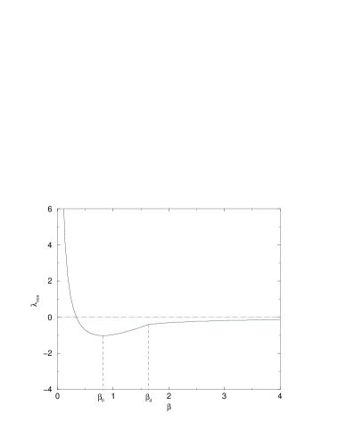
FIG. 1.: Left edge ($\lambda_{min}$) of the spectrum $\rho^{\infty}(\mu)$ as a function of the inverse temperature $\beta=1/T$ for $p=3$. $1/\beta_{d}$ is the dynamical glass transition temperature, whereas $1/\beta_{0}$ is the temperature at which $\lambda_{min}$ reaches its minimum value and is related to the damage spreading transition.

In fig.1 we have also indicated the dynamical transition temperature $T_{d}=1/\beta_{d}$. The density of states does not change qualitatively when the temperature crosses $T_{d}$: a fraction of negative eigenvalue is present at $T_{d}$ and vanishes for T going to zero. Therefore there is no sign of the dynamical transition in the behaviour of the density of states of instantaneous normal modes.

In summary, we have shown that the damage spreading transition seems to be related to a change in the local properties of the energy landscape seen by the system during the dynamical evolution. Conversely, the local properties of the energy landscape do not change qualitatively at the dynamical glass transition. At the dynamical glass transition the energy landscape seen by the system remains locally the same, whereas its global properties change and this can be observed by analysing the local properties of the free energy landscape.

V Conclusion

In this paper the Thouless, Anderson and Palmer approach to thermodynamics of mean field spin glasses has been generalised to dynamics. We have shown a procedure to compute dynamical TAP equations, which is the generalisation to dynamics of the $\frac{1}{d}$ ($d$ being the spatial dimension) expansion developed by A. Georges and S. Yedidia [26]. This method has been applied to the p-spin spherical model. In this context we have focused on the interpretation of the dynamics as an evolution in the free energy landscape.

We have shown that at finite times the dynamics cannot be represented as a gradient descent in the free energy landscape, because the reaction term in the dynamical TAP equation is non-Markovian.
However, the long-time dynamics can be interpreted as an evolution in the free energy landscape. Actually, for initial conditions belonging to stable TAP states the long-time evolution of local magnetisations coincides with a gradient descent in the free energy landscape with an extra spherical multiplier and extra magnetic fields going to zero at large times. For random initial conditions the local magnetisations vanish asymptotically because at any finite time two different typical noise histories bring the system in two completely uncorrelated configurations [37]. However, also in this case, a description of the long-time dynamics as an evolution in the free energy landscape makes sense, providing that the effects due to the spreading of the dynamical probability measure are separated from the slow motion of the system. In particular we have explicitly shown that slow dynamics is due to the motion in the flat directions of the free energy landscape in presence of a vanishing source of drift.
These results clarify and strengthen the relationship between long-times dynamics and local properties of the free energy landscape, which was already found in [9, 11, 20, 43].
Moreover we have shown that the local properties of the energy landscape seen during the dynamical evolution do not change qualitatively at the dynamical glass transition but at a higher temperature $T_{0}$, which is related to the damage spreading transition [22]. This indicates that at the dynamical glass transition the energy landscape seen by the system remains locally the same, whereas its global properties change and this can be observed by analysing the local properties of the free energy landscape.

Finally, we remark that there is still an important question which remains open and which has been clarified only for the zero temperature dynamics of the p-spin spherical model [12]: even if it is known that the TAP states having flat directions in the free energy landscape dominate the off-equilibrium dynamics, it is not clear why starting from a random initial condition the system goes toward these states. The dynamical TAP equations are strongly non-Markovian for any finite time. This result suggests that the matching between a certain initial condition (e.g. a random initial condition) and the asymptotic regime (slow dynamics at the threshold level) cannot be explained in terms of the static free energy and is a purely dynamical problem.

We conclude noticing that the formal analogies (due to the superspace notation) between static and dynamic free energy let us hope that the study performed in this article can be extended also to the cases in which an analytical solution is not available (finite dimensional system), but the symmetry properties of the asymptotic solution are known [44]. We are currently working in this direction.
Furthermore the dynamical TAP approach developed in this paper could be useful for the study of barrier crossing and instantons in the dynamics of mean field models [35].
Acknowledgments: I am deeply indebted to L. F. Cugliandolo, J. Kurchan and R. Monasson for numerous, helpful and thorough discussions on this work. I wish also to thank S. Franz and M. A. Virasoro for many interesting discussions on the asymptotic solution analysed in section III.B.2. I am particularly grateful to R. Monasson for his constant support and for a critical reading of the manuscript.

A Initial condition

We take as initial condition a fixed configuration $\{s_{i}^{0}\}$; therefore in the Martin-Siggia-Rose functional (27) one has only to integrate on paths such that $\{s_{i}(t=0)=s_{i}^{0}\}$. We impose this constraint by adding to the action (28) the term:

$$-\int dt\delta(t)\hat{s_{i}}(t)(s_{i}(t)-s_{i}^{0})\quad.$$ (A1)

This extra term has only two effects within the superspace formulation of dynamics: changes the operator $D$ and the (super)magnetic field $H_{i}$ in:

$$D^{in}=-2\frac{\partial^{2}}{\partial\theta\partial\overline{\theta}}-2\theta\frac{\partial^{2}}{\partial\theta\partial t}+\frac{\partial}{\partial t}+\delta(t)\qquad,\qquad H_{i}^{in}=H_{i}-\delta(t)s_{i}^{0}$$ (A2)

This replacement does not affect the derivation of dynamical TAP equations; then taking care of the initial condition leads only to replace $D$ with $D^{in}$ and $H_{i}$ with $H_{i}^{in}$ in the dynamical TAP equations (51 ) and (53). This corresponds to replace $\frac{\partial}{\partial t}$ with $\frac{\partial}{\partial t}+\delta(t)$ in equations (59) and (61) and to add to equation (63) the term $\delta(t)(m_{i}(t)-s_{i}^{0})$.
These new terms fix the initial condition on magnetisations: $m_{i}(t=0)=s_{i}^{0}$ and enforce the equality $C(t,0)=Q(t,0)$. This last condition is already expected on physical grounds because the thermal noise is not relevant at time $t=0$, therefore $\sum_{i=1}^{N}\left<s_{i}(t)s_{i}(0)\right>=\sum_{i=1}^{N}\left<s_{i}(t)\right>s_{i}(0)$.
We note that if we do not fix any particular initial condition, but we take as initial condition for the dynamical measure an uniform average over all possible configurations as in [9], then we find that the local magnetisations, the spherical multiplier, the correlation and the response functions fulfil (59), (61), (63) and (65) without the boundary condition on $C$. In this case the equations on the local on magnetisations are trivially satisfied because $m_{i}=0$ for every time $t$.

B INM

In this Appendix we show a standard way to compute the density of states of ${\mathbf{E}}$:

$$E_{i,j}=\frac{p(p-1)}{p!}\sum_{i_{3}\neq\dots\neq i_{p}}J_{i,j,i_{3},\dots,i_{p}}s_{i_{3}}\cdots s_{i_{p}}\quad,$$ (B1)

where $\{s_{i}(t)\}$ is an instantaneous dynamical configuration.
The spectral properties of ${\mathbf{E}}$ can be obtained through the knowledge of the resolvent $G(\mu+i\epsilon)$, that is the trace of $((\mu+i\epsilon){\mathbf{1}}-{\mathbf{E}})^{-1}$ [45]. Denoting the average over disorder by $\overline{(\cdot)}$ and the average over instantaneous configurations at time $t$ by $\left<\cdot\right>$, the mean density of states reads

$$\rho(\mu;t)=-\frac{1}{\pi}\lim_{\epsilon\to 0^{+}}\hbox{\rm Im}\;\overline{\left<G(\mu+i\epsilon)\right>}\quad.$$ (B2)

The averaged resolvent is then written as the propagator of a replicated Gaussian field theory [45]

$$\overline{G(\mu+i\epsilon)} = \lim_{n\rightarrow 0}\frac{-i}{Nn}\int\prod_{i}d\vec{\phi}_{i}\sum_{k=1}^{N}\vec{\phi}_{k}^{\;2}\overline{\left<\exp(L(s_{i}(t),\mu))\right>}$$ (B3)

$$\hbox{\rm where}\quad L(s_{i}(t),\mu) = \sum_{i=1}^{N}\frac{i}{2}(\mu+i\epsilon)\vec{\phi}_{i}^{\;2}-\sum_{i,j=1}^{N}\frac{i}{2}E_{i,j}\vec{\phi}_{i}\cdot\vec{\phi}_{j}\quad.$$ (B4)

Replicated fields $\vec{\phi}_{i}$ are $n$-dimensional vector fields attached to each site $i$. The average over the instantaneous dynamical configurations can be written in terms of Martin-Siggia-Rose functional [32]:

$$\left<\exp(L(s_{i}(t),\mu))\right> = \int\prod_{i=1}^{N}{\cal D}s_{i}{\cal D}\hat{s}_{i}\exp\left[L(s_{i},\mu)+S_{MSR}(s_{i},\hat{s}_{i})\right]$$ (B5)

$$S_{MSR}(s_{i},\hat{s}_{i}) = \int_{0}^{+\infty}dt\sum_{i=1}^{N}-\hat{s}_{i}\left(\frac{ds_{i}}{dt}+\frac{\partial H}{\partial s_{i}}-T\hat{s_{i}}\right)\quad,$$ (B6)

where we do not write the “ghosts” fields because we take the Ito convention.
Within the Martin-Siggia-Rose approach the average over the couplings is a simple Gaussian integral. Then we find that the total action is equal to:

$$S(s_{i},\hat{s}_{i},\phi_{i}^{a},t)=\sum_{i=1}^{N}\frac{i}{2}(\mu+i\epsilon)\vec{\phi}_{i}^{\;2}+\int_{0}^{+\infty}dt\sum_{i=1}^{N}-\hat{s}_{i}\left(\frac{ds_{i}}{dt}-T\hat{s_{i}}+\lambda s_{i}\right)+$$ (B7)

$$+\frac{1}{4N^{p-1}}\sum_{i_{1}\neq\cdots\neq i_{p}}\left[\int dt^{\prime}\left(\hat{s}_{i_{1}}s_{i_{2}}\cdots s_{i_{p}}+\cdots+s_{i_{1}}\cdots s_{i_{p-1}}\hat{s}_{i_{p}}+\frac{i}{2}\sum_{l\neq m}O_{l,m}^{t}\right)\right]^{2}\quad,$$ (B8)

where $O_{l,m}^{t}$ is symmetric under the exchange of $l$ and $m$ and is equal to:

$$O_{l,m}^{t}(t^{\prime}) = \delta(t^{\prime}-t)\sum_{a=1}^{n}s_{i_{1}}(t^{\prime})\cdots s_{i_{l-1}}(t^{\prime})\phi_{i_{l}}^{a}s_{i_{l+1}}(t^{\prime})\cdots s_{i_{m-1}}(t^{\prime})\phi_{i_{m}}^{a}s_{i_{m+1}}(t^{\prime})\cdots s_{i_{p}}(t^{\prime})\qquad(l<m)$$ (B9)

$$O_{l,m}^{t}(t^{\prime}) = 0\qquad l=m\quad.$$ (B10)

The action (B7) depends on $s_{i},\hat{s}_{i},\phi_{i}^{a}$ only through

$$C(t,t^{\prime})=\frac{1}{N}\sum_{i=1}^{N}s_{i}(t)s_{i}(t^{\prime})\quad R(t,t^{\prime})=\frac{1}{N}\sum_{i=1}^{N}s_{i}(t)\hat{s}_{i}(t^{\prime}) \quad D(t,t^{\prime})=\frac{1}{N}\sum_{i=1}^{N}\hat{s}_{i}(t)\hat{s}_{i}(t^{\prime})$$ (B11)

$$K_{a}(t)=\frac{1}{N}\sum_{i=1}^{N}s_{i}(t)\phi_{i}^{a}\quad \hat{K}_{a}(t)=\frac{1}{N}\sum_{i=1}^{N}\hat{s}_{i}(t)\phi_{i}^{a} \quad Q_{a,b}=\frac{1}{N}\sum_{i=1}^{N}\phi_{i}^{a}\phi_{i}^{b}\quad.$$ (B12)

In the large-N limit the functional integral giving the resolvent $G$ is dominated by a saddle point contribution.
The action (B7) is invariant when one changes $\vec{\phi}\rightarrow-\vec{\phi}$, therefore we take $K_{a}(t)=0$ and $\hat{K}_{a}(t)=0$. With this choice the saddle point equations on $K_{a}(t)$ and $\hat{K}_{a}(t)$ are trivially satisfied.
The saddle point equations on $C(t,t^{\prime})$, $R(t,t^{\prime})$ and $D(t,t^{\prime})$ are the usual ones [9].
Using the identity

$$-\delta_{a,b}=\frac{1}{N}\sum_{i=1}^{N}<<\phi_{i}^{a}\frac{\partial S}{\partial\phi_{i}^{b}}>>\quad,$$ (B13)

where $<<\cdot>>$ means the average over $s_{i},\hat{s}_{i},\phi_{i}^{a}$ (with weight $\exp(S)$), it is easy to obtain the saddle point equation on $Q_{a,b}$:

$$\frac{1}{2}p(p-1)C(t,t)^{p-2}\sum_{c=1}^{n}Q_{b,c}Q_{a,c}-i(\mu+i\epsilon)Q_{a,b}-\delta_{a,b}=0\quad.$$ (B14)

It is well known that in the computation of the density of states the replica symmetric saddle point gives the leading contribution. Therefore we take $Q_{a,b}=q\delta_{a,b}$.
The spherical constraint fixes $C(t,t)=1$, then from the saddle point equation on $q$ we get $q=\frac{i\mu+\sqrt{2p(p-1)-\mu^{2}}}{p(p-1)}$.
The density of states of $\mathbf{E}$ is obtained from (B2):

$$\rho(\mu;t)=\frac{1}{\pi}\Re(q)=\frac{1}{\pi p(p-1)}\sqrt{2p(p-1)-\mu^{2}}$$ (B15)

which is the Wigner semi-circle law. As expected this density does not depend on $t$. The only dependence on time for the density of states of the energy Hessian comes from $\frac{\lambda(t)}{\beta}$, which translates the centre of the semi-circle (see eq. (90)).

REFERENCES

-
[1]
For a recent review, see :
J.P. Bouchaud, L. Cugliandolo, M. Mézard, J. Kurchan, “Out of equilibrium dynamics in spin-glasses and other glassy systems”, A.P. Young editor, World Scientific, Singapore (1997) and references therein. - [2] See for instance many contributions in: “Landscape Paradigms in Physics and Biology”, Physica D 107, 117-437 (1997).
- [3] M. Mézard, G. Parisi and M. Virasoro, Spin Glass Theory and Beyond (1987) (Singapore: World Scientific).
- [4] D. J. Thouless, P. W. Anderson and R. G. Palmer, Phil. Magazine 35, 593 (1977).
- [5] D. Sherrington and S. Kirkpatrick, Phys. Rev. Lett. 35, 1972 (1975).
- [6] C. De Dominicis and A.P. Young, J. Phys. A 16, 2063 (1983).
- [7] M. Mézard, G. Parisi and M. Virasoro, Europhys. Lett. 1, 77 (1986).
- [8] G. Parisi, Phys. Lett. A 73, 154 (1979), J. Phys. A 13, L115 (1980), ibid 13, 1101 (1980), ibid 13, 1887 (1980).
- [9] L.F. Cugliandolo and J. Kurchan, Phys. Rev. Lett. 71, 173 (1993) and Phil. Mag. B 71, 501 (1995).
- [10] R. Monasson, Phys. Rev. Lett. 75, 2847 (1995).
- [11] S. Franz and G. Parisi, J. Phys. (France) I 5, 1401 (1995).
- [12] J. Kurchan and L. Laloux J. Phys. A 29, 1929 (1996).
- [13] T. R. Kirkpatrick and P. G. Wolynes, Phys. Rev. A 34, 1045 (1986); T. R. Kirkpatrick and D. Thirumalai, Phys. Rev. Lett 58, 2091 (1987);T. R. Kirkpatrick and D. Thirumalai, Phys. Rev. B 36, 5388 (1987); T. R. Kirkpatrick and D. Thirumalai and P. G. Wolynes, Phys. Rev. A 40, 1045 (1989).
- [14] G. Parisi and M. Mézard, Phys. Rev. Lett. 82, 747 (1999).
- [15] J. P. Bouchaud, L. F. Cugliandolo, J. Kurchan and M. Mézard, Physica A 226, 243 (1996).
- [16] W. Götze, J. Phys. Condens. Matter 11, A1-A45 (1999).
- [17] J. Kurchan, G. Parisi and M. A. Virasoro, J. Phys I (France) 3, 1819 (1993).
- [18] A. Crisanti and H.-J. Sommers, J. Phys. I France 5, 805 (1995).
- [19] A. Crisanti, H. Horner and H.-J. Sommers, Z. Phys. B 92, 257 (1993).
- [20] A. Barrat, R. Burioni and M. Mézard , J. Phys. A 29, L81 (1996).
- [21] T. Keyes J. Phys. Chem. A 101, 2921 (1997).
- [22] M. Heerema and F. Ritort J. Phys. A: Math. Gen. 31, 8423 (1998) and cond-mat/9812346.
- [23] H. J. Sommers, Z. Phys. B 31, 301 (1978); C. De Dominicis, Phys. Rep. B 67, 37 (1980); H. Rieger, Phys. Rev. B 46, 14655 (1992) .
- [24] J. M. Cornwall, R. Jackiw and E. Tomboulis, Phys. Rev. 10, 2428 (1974); R. W. Haymaker, Riv. Nuovo Cimento 14, 1 (1991).
- [25] T. Plefka, J. Phys. A 15, 1971 (1982).
- [26] A. Georges and J.S. Yedidia, J. Phys. A 24, 2173 (1991).
- [27] D.J. Gross and M. Mézard, Nuc. Phys. B 240, 431 (1984).
- [28] A. Barrat cond-mat/9701031, unpublished.
- [29] A. Crisanti and H.-J. Sommers, Z. Phys. B 87, 341 (1992).
- [30] J. Kurchan, J. Phys. France 2, 1333 (1992); S. Franz and J. Kurchan, Europhys. Lett. 20, 197 (1992).
- [31] J. Zinn-Justin, Quantum Field Theory and Critical Phenomena , Clarendon Press 1997.
- [32] P.C. Martin, E.D. Siggia and H.A. Rose, Phys. Rev. A 8, 423 (1978); C. de Dominicis and L. Peliti, Phys. Rev. B 18, 353 (1978).
- [33] E. Gozzi, Phys. Lett. 143, 183 (1984).
- [34] H. Sompolinsky and A. Zippelius, Phys. Rev. B 25, 6860 (1982).
- [35] L. B. Ioffe and D. Sherrington, Phys. Rev. B 57, 7666 (1998). A. V. Lopatin and L. B. Ioffe, Phys. Rev. B 60, 6412 (1999); cond-mat/9907135.
- [36] J. P. Bouchaud, J. Phys. I (France) 2 1705 (1992).
- [37] A. Barrat, R. Burioni and M. Mézard, J. Phys. A 29, 1311 (1996).
- [38] S. Franz and M. A. Virasoro, condmat/9907438.
- [39] G. Biroli, S. Franz and M. A. Virasoro, in preparation.
- [40] L. F. Cugliandolo and D. S. Dean, J. Phys. A 28, 4213 (1995).
- [41] A. Bray and M. A. Moore, J. Phys. C: Solid State Phys. 12, L441 (1979).
- [42] M. L. Metha, Random Matrices and the Statistical theory of Energy Levels (1967) (New York: Academic).
- [43] G. Biroli and R. Monasson, J. Phys. A 31, L391 (1998).
- [44] L.F. Cugliandolo and J. Kurchan, Physica A 263, 242 (1999).
- [45] D.J. Thouless, Physics Reports 13, 93 (1974); Mesoscopic quantum physics, Les Houches session LXI, (Elsevier Science, 1995).