Kinks in the discrete sine-Gordon model
with Kac-Baker long-range interactions

Abstract

We study effects of Kac-Baker long-range dispersive interaction (LRI) between particles on kink properties in the discrete sine-Gordon model. We show that the kink width increases indefinitely as the range of LRI grows only in the case of strong interparticle coupling. On the contrary, the kink becomes intrinsically localized if the coupling is under some critical value. Correspondingly, the Peierls-Nabarro barrier vanishes as the range of LRI increases for supercritical values of the coupling but remains finite for subcritical values. We demonstrate that LRI essentially transforms the internal dynamics of the kinks, specifically creating their internal localized and quasilocalized modes. We also show that moving kinks radiate plane waves due to break of the Lorentz invariance by LRI.

I Introduction

The effects of long-range dispersive interactions (LRI’s) on the dynamics and thermodynamics of soliton-bearing systems have attracted a great deal of interest in the past decade [1, 2, 3, 4, 5, 6, 7, 8, 9, 10, 11, 12, 13, 14, 15, 16, 17, 18, 19, 20, 21, 22]. Such attention is due to the fact that in realistic physical systems the interparticle forces are always long-ranged to some extent, and if the range of LRI’s exceeds some critical value, they change soliton features qualitatively. In particular, the competition between short-range and long-range interactions in anharmonic chains [1, 2, 3, 4, 5, 6, 7, 8, 9] and nonlinear Schrödinger (NLS) models [10, 11, 12, 13, 14] brings into existence several types of the soliton states. In the nonlocal discrete NLS model two types of stable soliton states can coexist at the same excitation number [12]. In other words, there occurs a bistability phenomenon with a possibility of controlled switching between states [14]. Besides, the power law LRI manifests itself in algebraic soliton tails [12, 8, 9] and can give rise to an energy gap between the spectra of plane waves and the soliton states [9].

In the present paper we consider the effects of LRI’s in discrete Klein-Gordon (KG) models. These models were successfully used in investigations of a number of physical phenomena such as dislocations in solids, charge-density waves, adsorbed layers of atoms, domain walls in ferromagnets and ferroelectrics, crowdions in metals, and hydrogen-bonded molecules (see the review paper [23] for references). As it is known [16, 23] the interparticle interactions in many of these systems are substantially long-ranged.

In the assumption of the harmonic interaction between particles the dimensionless Hamiltonian of the discrete KG model can be written in the form

$$H = \sum_{n}\biggl{\{}\frac{1}{2}\Bigl{(}\frac{du_{n}}{dt}\Bigr{)}^{2}+V(u_{n})$$ (1)

$$+ \frac{1}{2}\sum_{m>n}J_{m,n}(u_{m}-u_{n})^{2}\biggr{\}}\;,$$ (2)

where $u_{n}$ is the displacement of the $n$-th particle from its equilibrium position and $J_{m,n}$ is the coupling constant between particles $n$ and $m$.

As far as we know, until now there was only one investigation [16] of the KG model with the power law LRI. It was shown that the asymptotics of the kink shape as well as the interaction energy of the kinks are power law and, because of this, the dependence of the Peierls-Nabarro barrier versus the atom concentration is similar to the “devil’s staircase”.

But KG models with the exponential law (usually called Kac-Baker) LRI

$$J_{m,n}=J(e^{\alpha}-1)e^{-\alpha|m-n|}\;$$ (3)

were believed to have been investigated in an exhaustive fashion [17, 18, 19, 20, 21, 22]. As early as 1981, Sarker and Krumhansl found [17] an analytical kink solution for the $\phi^{4}$ model. The width and the energy of the kinks were found to increase indefinitely as $\alpha$ decreases. An important role of the Kac-Baker LRI in thermodynamics of the system was also shown. Within the decade Woafo et al. considered in a series of papers [18, 19, 20] the discreteness effects in the same model. They have shown that the Peierls-Nabarro barrier vanishes as $\alpha\to 0$.

More recently the sine-Gordon (SG) model

$$V(u_{n})=1-\cos u_{n}\;$$ (4)

with Kac-Baker LRI (3) has been studied [21, 22] and all results of Ref. [17] have been extended to this model. An implicit form for the kinks has been obtained and the kink energy and width have been found to grow to infinity as $\alpha\to 0$ in Ref. [21]. The thermodynamics of the system has been thereafter studied in Ref. [22].

Thus, the investigations performed in Refs. [17, 18, 19, 20, 21, 22] give the impression that the Kac-Baker LRI always results, in the limit $\alpha\to 0$, into infinite increasing of the kink width (and, therefore, vanishing of the Peierls-Nabarro barrier). However, closer inspection shows that this conclusion is proper for the case $J>0.5$ only.

In the present paper we explore the effects of the Kac-Baker LRI in the discrete sine-Gordon model (1)-(4) further so that we could cover the case $J<0.5$. What is more, we investigate the internal kink dynamics and the radiation of moving kinks.

The paper is organized as follows. In Sec. II we derive the equation of motion of the system in the continuum limit using the technique of pseudo-differential operators. Then, in Sec. III we solve this equation and obtain an implicit analytical form of the kink solution for arbitrary values of $\alpha$ and $J$. Turning back to the discrete case we calculate the form of the kinks numerically and compare it with the analytical solution. We show that in the case of $J(e^{\alpha}+1)<1$ the kinks are intrinsically localized. The calculation of the Peierls-Nabarro barrier as a function of $\alpha$ and $J$ finishes the section. It turns out that the Peierls-Nabarro barrier vanishes in the limit $\alpha\to 0$ for $J>0.5$ but remains finite for $J<0.5$. In Sec. IV we develop a variational approach to the internal kink dynamics and demonstrate that LRI strongly enhances creation of kink’s internal modes. Then we validate this result by direct numerical calculations. We show that similar to the non-sinusoidal Peyrard-Remoissenet potential [24, 25], the Kac-Baker LRI (3) with small $\alpha$ creates several kink’s internal modes. By this means our results support the recent conclusion of Kivshar et al. [26] that “the internal mode is a fundamental concept for many nonintegrable soliton models”. Moreover, we show that for large values of $J$, for which kink’s internal modes do not exist, the Kac-Baker LRI gives rise to pronounced quasilocalized modes inside of the phonon spectrum. In Sec. V we show that due to break of the Lorentz invariance by LRI, there are no stationary moving kinks in the system; arbitrary moving kink will radiate plane waves with the wavelength proportional to its velocity. In Sec. VI we summarize and discuss the obtained results.

II Equations of motion

The Hamiltonian (1)-(4) generates the equation of motion

$$\frac{d^{2}u_{n}}{dt^{2}}-\sum_{m\neq n}J_{m,n}(u_{m}-u_{n})+\sin u_{n}=0\;.$$ (5)

To obtain its solution analytically we pass to the continuum limit treating $n$ as a continuous variable $n\to x=an$, where $a$ is the distance between particles. Thus, using

$$u_{n}(t)\to u(x,t)\quad,\quad u_{m}(t)\to e^{(am-x)\partial_{x}}u(x,t)\;$$ (6)

and keeping formally all terms in the Taylor expansion of $e^{(am-x)\partial_{x}}$, we can cast Eq. (5) in the operator form

$$\partial^{2}_{t}u-\frac{J(e^{\alpha}+1)\sinh^{2}(a\partial_{x}/2)}{\sinh^{2}(\alpha/2)-\sinh^{2}(a\partial_{x}/2)}u+\sin u=0\;,$$ (7)

where $\partial_{x}$ and $\partial_{t}$ are the derivatives with respect to $x$ and $t$, respectively, and the identity

$$\sum_{m\neq 0}e^{-\alpha|m|+am\partial_{x}}\equiv\frac{\cosh(a\partial_{x})-e^{-\alpha}}{\cosh(\alpha)-\cosh(a\partial_{x})}\;$$ (8)

has been used.

In the approximation $\sinh(a\partial_{x}/2)\approx a\partial_{x}/2$ the equation of motion (7) takes on the form

$$\partial^{2}_{t}u-\frac{\partial_{z}^{2}}{1-\sigma^{2}\partial_{z}^{2}}u+\sin u=0\;,$$ (9)

where $z=x/(a\xi)$ with

$$\xi=\frac{\sqrt{J(e^{\alpha}+1)}}{2\sinh(\alpha/2)}\qquad\mbox{and}\qquad\sigma^{2}=\frac{1}{J(e^{\alpha}+1)}\;.$$ (10)

Here the parameter $\xi$ presents a measure for the soliton width — the continuum approximation should be good for large enough values of $\xi$.

Acting on Eq. (9) by the operator $(1-\sigma^{2}\partial_{z}^{2})$ one can write the equation of motion in the differential form

$$u_{tt}-u_{zz}+\sin u=\sigma^{2}u_{zztt}+\sigma^{2}(\sin u)_{zz}\;,$$ (11)

which coincides with the equation derived in Ref. [21]. The authors of that paper found the form of the moving kink solution neglecting the term $u_{zztt}$. Thus they have found in fact an exact solution for immobile kinks but approximate for moving ones. In Sec. V we will show that the term $u_{zztt}$ is responsible for the non-perturbative radiation of the kink. Indeed, due to break of the Lorentz invariance by LRI there are no stationary moving kinks in the system — moving kinks always radiate and eventually stop. It is why in the next section we consider the immobile kinks only and write their exact shape in to some extent more simple and general form than that given in Ref. [21].

III Kink’s static properties

A Analytical kink solution

In this section we obtain the immobile ($\partial^{2}_{t}u=0$) kink solution of Eq. (9). Denoting this solution as $\phi(y;B)$, where

$$y=\frac{z}{\sigma}=\frac{2}{a}\sinh\biggl{(}\frac{\alpha}{2}\biggr{)}x\;$$ (12)

and

$$B^{2}=1+\frac{1}{\sigma^{2}}=1+J(e^{\alpha}+1)\;,$$ (13)

one can see that Eq. (9) takes on the form

$$\frac{\partial_{y}^{2}}{1-\partial_{y}^{2}}\phi(y;B)=\frac{\sin\phi}{B^{2}-1}\;.$$ (14)

Using a new variable $v=\sin(\phi/2)$ one can rewrite it in the polynomial form

$$(1-v^{2})(B^{2}-2v^{2})v_{yy}$$ (15)

$$+v(B^{2}-4+2v^{2})v_{y}^{2}=v(1-v^{2})^{2}\;,$$ (16)

and multiplying by $(B^{2}-2v^{2})/(1-v^{2})^{2}$ one can cast it in the form of the equation of motion of certain Hamiltonian system with the Hamiltonian

$$h=\frac{(B^{2}-2v^{2})^{2}}{2(1-v^{2})}v_{y}^{2}-\frac{1}{2}v^{2}(B^{2}-v^{2})\;.$$ (17)

Imposing the kink’s boundary conditions ($v_{y}\to 0$ when $v\to 0$) we arrive at the constraint $h=0$. Thus we obtain the equation

$$v_{y}^{2}=\frac{v^{2}(1-v^{2})(B^{2}-v^{2})}{(B^{2}-2v^{2})^{2}}\;,$$ (18)

which after integration gives the kink solution of the form

$$\pm(y-y_{0}) = \frac{B}{2}\log\biggl{(}\frac{1+B\mu}{1-B\mu}\biggr{)}+\log\biggl{(}\frac{1-\mu}{1+\mu}\biggr{)}$$ (19)

$$= \sum_{m=1}^{\infty}\frac{B^{2m}-2}{2m-1}\mu^{2m-1}\;,$$ (20)

where a new variable

$$\mu=\sqrt{\frac{1-v^{2}}{B^{2}-v^{2}}}\;$$ (21)

is introduced. Turning back to the function $\phi(y;B)$ we obtain an exact form of the kink (positive sign in Eq. (19)) or antikink (negative sign) centered at $y_{0}$:

$$\phi(y;B)=2\arcsin\biggl{(}\sqrt{\frac{1-B^{2}\mu^{2}}{1-\mu^{2}}}\biggr{)}\;,$$ (22)

where the dependence of $\mu$ on $y$ is determined by Eq. (19).

It can be checked that in the nearest-neighbors interaction (NNI) limit ($B\to\infty$) the solution reduces to the ordinary SG kink or antikink form

$$u(z)=4\arctan(\exp(\pm(z-z_{0})))\;,$$ (23)

where we have used the variables $u(z)$ and $z$ defined in the previous section.

Looking at Eq. (19) one can see that near the center of the kink, where $\mu$ is small, the first order term in the Taylor series vanishes at $B=\sqrt{2}$. In this case the derivative $d\mu/dy=\pm 1/2\mu^{2}$ goes to infinity in the center ($\mu\to 0$) of the kink. It means that the slope of the kink becomes vertical for $B=\sqrt{2}$ (see Fig. 1). If $B<\sqrt{2}$ the slope of the kink assumes negative values and the solution (22) becomes ${\cal S}$-shaped (multivalued) and thus loses its physical meaning.

FIG. 1.: The kink shape predicted analytically for different values of the range of LRI: it is usual in the NNI limit ($B=\infty$, full line), has the vertical slope in the critical case ($J(e^{\alpha}+1)=1$ or $B=\sqrt{2}$, dotted line), and is multivalued (${\cal S}$-shaped) in the supercritical cases of $B=1.2$ (dashed line) and $B=1.1$ (long-dashed line).

Thus, returning to the initial physical parameters $J$ and $\alpha$ we can state that there exists a critical value of $J$ in the system: if $J>0.5$ the value of $B$ always exceeds $\sqrt{2}$ and the form of the kink does not change drastically with $\alpha$ (see Fig. 2-a). It was this case which was studied in details in Refs. [21, 22]. But if $J<0.5$ there is some critical value of $\alpha$ for which $B=\sqrt{2}$ and the transition from usual kinks to ${\cal S}$-kinks occurs when $\alpha$ decreases (see Fig. 2-b). And now an interesting question should be raised: what is a physical single-valued analogue of the ${\cal S}$-kink in the discrete case?

B Numerical results

The best remedy to answer the above question is to solve Eq. (5) numerically. Since for a static solution Eq. (5) turns itself into a system of $N$ nonlinear algebraic equations (where $N$ is a number of particles), it is convenient to use the Newton-Raphson iterations. To avoid perturbations due to boundary effects (we use a chain with fixed ends) the value of $N$ was chosen large enough (typically $N=500$, but it has been extended to 1000 for broad kinks at small $\alpha$ and big $J$). The choice of the initial kink form for zeroth iteration is not very important since for the given problem the Newton-Raphson iterations are very stable (but to be specific we used Eq. (23) for this purpose). To obtain a stationary kink shape with the equilibrium positions $u_{n}^{\rm eq}$ of the particles in a chain we usually performed 7–20 iterations.

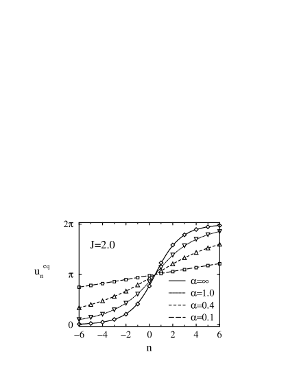
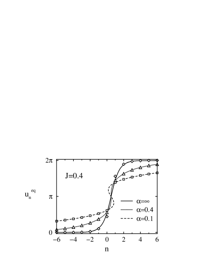
FIG. 2.: The comparison of the kink shape predicted analytically with that found numerically. Two cases must be distinguished: a) $J>0.5$ for which the kink width increases indefinitely with decreasing of the $\alpha$; b) $J<0.5$ for which the kink width remains finite with decreasing of $\alpha$.

In Figs. 2-3 we compare the form of the kinks found numerically for different $J$ and $\alpha$ with the solution (19)-(22). One can see that at small $\alpha$ the agreement between them is excellent for all values of $J$. The only difference is that one should cut out the unphysical part of the ${\cal S}$-kink and replace it with a vertical slope to obtain the form of the kink in the discrete case (see Fig. 3). In our opinion this result can be understood by reference to a two-component kink structure. Indeed, as it was shown in Refs. [5, 6] for the anharmonic chain with the Kac-Baker LRI between particles, the existence of two length scales results into two-component soliton structure, where the short-range component is dominant in the center of the soliton, while the long-range component (which can be properly described in the continuum approximation by Eq. (14)) is dominant in the tails.

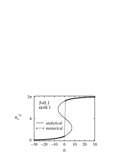
FIG. 3.: The kink shape at small $J$ and $\alpha$: instead of the predicted analytically multivalued ${\cal S}$-shaped kink we obtain numerically the intrinsically localized kink.

FIG. 4.: The dependence of the energy $E_{PN}$ of the Peierls-Nabarro barrier on the range $\alpha$ of LRI for different values of $J$. The barrier vanishes in the limit $\alpha\to 0$ for $J\geq 0.5$ but remains finite for $J<0.5$.

Thus, now we can conclude that in the discrete SG model the LRI affects the kinks in two opposite ways in relation to the value of $J$. When $J>0.5$ the increasing of the range of LRI causes the increasing of the kink width in agreement with the conclusion of Ref. [21]. But for $J<0.5$ the kinks become intrinsically localized as $\alpha\to 0$. In the latter case the form of the kink is perfectly described by the ${\cal S}$-kink in the tails with a vertical slope in the center.

Numerical calculations show that in both cases the kink energy monotonically grows to infinity when $\alpha$ decreases to zero. But the behavior of the Peierls-Nabarro barrier (defined as an energy difference of the kink centered on a particle and the kink centered between particles) completely correlates with the behavior of the kink form (see Fig. 4). When (for $J>0.5$) the kink width grows in the limit $\alpha\to 0$, the Peierls-Nabarro barrier vanishes. But when (for $J<0.5$) the kink becomes intrinsically localized in this limit, the Peierls-Nabarro barrier remains finite.

IV Kink’s internal modes

In the previous section we were concentrating upon the static properties of the kinks. But a considerable interest is also attracted to the phonon spectrum affected by the presence of the kink. It is common knowledge that the influence of the kink is to some extent similar to that of the impurity affecting the phonon spectrum in a solid. Namely, not only quantitative changes in the spectrum, but qualitative ones consisting in emerging the localized modes with frequencies lying beyond the phonon band are to be expected and present special interest [25, 26, 27, 28, 29, 30].

There should be distinguished localized internal modes from the localized translational mode. The low-frequency translational mode (which is in the continuum limit the Goldstone mode associated with the translational invariance) is universally present in an arbitrary KG model. Its frequency is closely associated with the Peierls-Nabarro barrier considered above, so we shall not focus much attention on this mode in what follows; instead, we shall consider in detail the internal modes. These latter play an important role in the kink dynamics because they can temporarily store energy taken away from the kink’s kinetic energy, which can later be restored again in the kinetic energy. This gives rise to resonant structures in kink interactions [31, 32, 33, 34].

The most extensively studied is the Rice internal mode [27] which can be visualized as an oscillation of the kink’s core width. Although this mode does not exist [28] in the usual continuum SG model (which is integrable), even small perturbation of the model brings it into the existence [25, 26]. In particular, the Rice mode exists in the discrete SG model with NNI [25]. But the discreteness just changes the dispersion of the system and the dispersive LRI under consideration affects it even greater. Thus, one might expect that the LRI will enhance the creation of the Rice internal mode in the system being considered. In the next subsection we recourse to a variational approach and show that this is so indeed. Then we investigate kink’s internal modes in more detail numerically. It turns out that at small $\alpha$ there can exist either several kink’s internal modes below the phonon spectrum or pronounced quasilocalized modes inside the phonon spectrum.

A Variational approach

When, as with the $\varphi^{4}$–model, the Rice internal mode is pronounced it can be properly described by a variational collective coordinates approach [27]. Proceeding from Eq. (8) and the identity

$$\sum_{n}\sum_{m>n}J_{m,n}(u_{m}-u_{n})^{2}\equiv-\sum_{n}u_{n}\sum_{m\neq n}J_{m,n}(u_{m}-u_{n})$$ (24)

one can pass to the continuum limit (6) and write the Hamiltonian (1) in the form

$$H = \frac{1}{2\sinh(\alpha/2)}\int_{-\infty}^{\infty}dy\biggl{\{}\frac{1}{2}\biggl{(}\frac{du}{dt}\biggr{)}^{2}+(1-\cos u)$$ (25)

$$- \frac{1}{2}u(y,t)\frac{J(e^{\alpha}+1)\partial_{y}^{2}}{1-\partial_{y}^{2}}u(y,t)\biggr{\}}\;,$$ (26)

where $y=2\sinh(\alpha/2)\,n$.

It should be emphasized that the Rice’s collective coordinates approach [27] cannot be used in our case. Indeed, choosing the trial function of the form $\phi(y/L(t);B)$, where $\phi(y;B)$ is the stationary kink solution (19)-(22) and $L(t)$ is a time-dependent variational parameter (so-called “effective kink width”), we are unable to integrate analytically the long-range part of the Hamiltonian (25).

Thus, we are forced to introduce another trial function. We call your attention to the fact (see Fig. 1) that the change of $B$ in the kink solution $\phi(y;B)$ changes a slope of the kink and its width as well. Therefore, to describe small-amplitude kink oscillations around its stationary form one can use equally well instead of Rice’s trial function a trial function of the form

$$u_{n}(t)=\phi(2\sinh(\alpha/2)\,n\,;\,b(t))\;,$$ (27)

where $\phi$ is determined by Eqs. (19)-(22) and $b(t)$ is the time-dependent variational parameter. Then, using that $\phi(y;b(t))$ is the solution of the equation

$$\frac{\partial_{y}^{2}}{1-\partial_{y}^{2}}\phi(y;b(t))=\frac{\sin\phi(y;b)}{b^{2}-1}\;,$$ (28)

the integrals appearing in Eq. (25) can be taken analytically:

$$U(b)=\int_{-\infty}^{\infty}dy(1-\cos\phi)=4b-2\log\biggl{(}\frac{b+1}{b-1}\biggr{)}\,,$$ (29)

$$V(b)=-\frac{1}{2}\int_{-\infty}^{\infty}dy\phi\sin\phi=2b+(b^{2}-1)\log\biggl{(}\frac{b+1}{b-1}\biggr{)}\,,$$ (30)

and

$$M(b) = \int_{-\infty}^{\infty}dy\biggl{(}\frac{d\phi}{db}\biggl{)}^{2}=\frac{2}{b^{2}-1}$$ (31)

$$\times \int_{0}^{1/b}d\mu\frac{\biggl{[}2b\mu+(b^{2}-1)\log\biggl{(}\frac{1+b\mu}{1-b\mu}\biggr{)}\biggr{]}^{2}}{(1-\mu^{2})\,(b^{2}-2+b^{2}\mu^{2})}\,,$$ (32)

where the last integral was taken analytically as well, yet its cumbersome expression prevents us from writing it down here in an explicit form. We just mention that $M(b)$ grows to infinity as $b\to\sqrt{2}$ and has the asymptotics

$$M(b)\simeq\frac{2\pi^{2}}{3b}+(12+\pi^{2})\frac{2}{3b^{3}}+(16+\frac{46}{45}\pi^{2})\frac{1}{b^{5}}+{\cal O}\biggl{(}\frac{1}{b^{7}}\biggr{)}$$ (33)

for big values of $b$.

Thus the effective Hamiltonian of the system takes on the form

$$H_{eff}=\frac{1}{2\sinh(\alpha/2)}\biggl{\{}\frac{1}{2}M(b)\biggl{(}\frac{db}{dt}\biggr{)}^{2}+W(b)\biggr{\}}\;,$$ (34)

where the potential energy of the kink

$$W(b) = U(b)+\frac{B^{2}-1}{b^{2}-1}\,V(b)\simeq E_{K}(B)$$ (35)

$$+ \frac{4B^{3}}{(B^{2}-1)^{2}}(b-B)^{2}+{\cal O}(b-B)^{3}\,,$$ (36)

as it would be expected, is minimal in the point $b=B\equiv\sqrt{1+J(e^{\alpha}+1)}$, where it equals to the energy

$$E_{K}(B)=6B+(B^{2}-3)\log\biggl{(}\frac{B+1}{B-1}\biggr{)}$$ (37)

of the stationary kink. The kink energy (37) was calculated first (although in a more bulky form) in Ref. [21].

For small deviations of $b$ from $B$ (in the harmonic approximation) the effective Hamiltonian (34) generates the equation of motion

$$\biggl{(}\frac{d^{2}}{dt^{2}}+\Omega^{2}\biggr{)}(b(t)-B)=0$$ (38)

being the equation of motion for the harmonic oscillator with the frequency

$$\Omega=\biggl{[}\frac{8B^{3}}{M(B)(B^{2}-1)^{2}}\biggr{]}^{1/2}\,,$$ (39)

whose dependence on $B$ is depicted on Fig. 5.

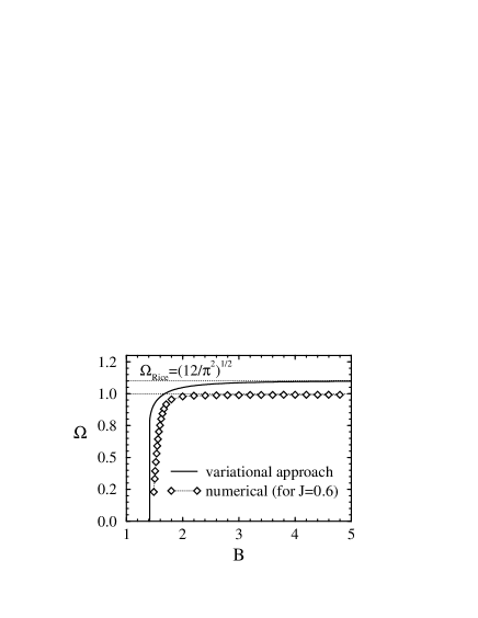
FIG. 5.: The dependence of the frequency $\Omega$ of the Rice’s kink internal mode on the parameter of the nonlocality $B=\sqrt{1+J(e^{\alpha}+1)}$: predicted analytically by Eq. 39 (full line) and found numerically for $J=0.6$ (diamonds).

Thus, a slightly excited kink will oscillate around its stationary shape with the frequency $\Omega$, depending upon the parameter $B$ which specifies the nonlocality of the system. When $B$ decreases (nonlocality grows) the frequency $\Omega$ also decreases ($\Omega\to 0$ when $B\to\sqrt{2}$). Although Eq. (39) is not fully precise even in the continuum limit (to improve it an interaction with phonons should be taken into account [28]) it is in a good agreement with the numerical calculations (see Fig. 5) which are described below.

B Numerical results

The exposed variational approach (even in a form complicated by introducing of several time-dependent parameters) permits one to investigate only a limited number of oscillatory modes. To overview rather the entity of the whole phonon spectrum one should deal with the initial set of the equations of motion (5). Specifically, when all the equilibrium positions $u_{n}^{\rm eq}$ of the particles in a chain with a kink become known by the method described in Sec. III B, we can study the spectrum of small-amplitude oscillations around this state by looking for a solution of Eq. (5) in the form

$$u_{n}=u_{n}^{\rm eq}+v_{n}\,e^{i\Omega t}\;.$$ (40)

We assume that the deviations $v_{n}$ of the particles from the kink shape are sufficiently small ($v_{n}\ll a$) and ignore all nonlinear terms in the equations of motion for $v_{n}$. Introducing this ansatz into Eq. (5), we obtain a system of linear equations that can be written in a matrix form

$$\hat{D}\vec{v}=\Omega^{2}\vec{v}\;,$$ (41)

where $\vec{v}\equiv\{v_{n}\}$ and a symmetric matrix $\hat{D}$ is the dynamical matrix of the lattice in the presence of a kink with the components:

$$D_{n,n} =2J+\cos u_{n}^{\rm eq}\;,$$ (42)

$$D_{n,m} =D_{m,n}=-J_{n,m}\;.$$ (43)

By virtue of the fact that the matrix $\hat{D}$ is symmetric all its eigenvalues are real. They give us the frequencies of the small-amplitude oscillations around the kink while the corresponding wavevectors describe the spatial profile of each mode. The eigenvalues and eigenvectors of the matrix $\hat{D}$ were calculated numerically using the Householder matrix reduction to tridiagonal form and the $QL$ diagonalization algorithm [35]. The obtained results are presented in Figs. 6 - 11. In the following discussion of these results, we assume that the reader is familiar with Ref. [25] where the basic features of the kink’s linear spectrum are comprehensively expounded.

FIG. 6.: Spectrum of small-amplitude excitations around a kink as a function of the coupling parameter $J$ for $\alpha=\infty$ and $\alpha=0.5$.

In Fig. 6 we compare the kink’s linear spectrum $\Omega(J)$ for $\alpha=0.5$ with the spectrum obtained in Ref. [25] for the NNI limit ($\alpha=\infty$). As it has there been shown, in the discrete SG model with the interaction between nearest neighbors aside from the low-frequency translational localized mode there exist (slightly expressed in the interval $0.27\lesssim J\lesssim 1.59$) the Rice internal mode. One can see from Fig. 6 that for $\alpha=0.5$ the situation remains qualitatively the same, except that the Rice mode becomes evidently pronounced. Thus, in agreement with the results of the variational approach, the LRI strongly enhances creation of the Rice mode (see also Fig. 5).

FIG. 7.: Spectrum of small-amplitude excitations around a kink as a function of the nonlocality parameter $\alpha$ for $J=0.6$.

Furthermore, when $\alpha$ yet decreases, there occur new qualitative phenomena. Foremost, additional localized internal modes are split out from the bottom of the phonon spectrum. This process is easily observable in Fig. 7 where the kink’s linear spectrum $\Omega$ as a function of $\alpha$ is plotted for $J=0.6$. One can see that the number of localized modes grows indefinitely as $\alpha$ vanishes. In particular, there are four localized modes at $\alpha=0.2$ (see Fig. 8-a) and seven at $\alpha=0.1$ (see Fig. 8-b). All the localized internal modes are best pronounced around $J\simeq 0.6$. Closer analytical examination of Eqs. (41)-(42) shows that all eigenstates are either symmetric or antisymmetric. One can state on the strength of the numerical calculations that the symmetric and antisymmetric states are always alternating, starting with the symmetric translational mode (Mode 1 in Fig. 9) and antisymmetric Rice mode (Mode 2 in Fig. 9).

FIG. 8.: Spectrum of small-amplitude excitations around a kink as a function of the coupling parameter $J$ for: a) $\alpha=0.2$ and b) $\alpha=0.1$.

Another interesting feature that appears in the kink’s linear spectrum at small $\alpha$ is that there exist an apparent transformation of the phonon spectrum (in the plane $\Omega-J$) along an imaginary line (let us call it “ridge”) which extends the localized internal modes inside the phonon spectrum in the direction of larger $J$ (see Fig. 8). This ridge is evidently parallel to the upper cut-off frequency of the phonon band, with the spectrum curves looking like essentially different left or right from the ridge. In the domain right to the ridge each symmetric eigenstate is equidistant from both nearest antisymmetric eigenstates. In the domain left to the ridge each symmetric eigenstate is paired with an appropriate antisymmetric eigenstate: their frequencies become almost coincident. The shapes of the symmetric and antisymmetric states in a pair are also in a close correlation: $v_{n}^{\rm a}\simeq\theta(n-n_{0})\,v_{n}^{\rm s}\,$, where $n_{0}$ is the position of the kink center and $\theta(x)$ is the Heaviside function. The ridge is shifted towards the upper cut-off frequency as $\alpha$ grows and completely disappears (or rather coincides with the upper edge of the phonon band) in the NNI limit ($\alpha=\infty$).

FIG. 9.: Example of the shape of the lowest localized modes: the translational mode (Mode 1), the Rice mode (Mode 2), and so on.

FIG. 10.: The shape of the delocalized and quasilocalized states inside the phonon band for $J=1.25$ and $\alpha=0.1$.

The most interesting phenomenon however concerns the shape of the eigenstates in the vicinity of the ridge (see Fig. 10). One can see that both above (e.g., mode 40 in Fig. 10) and below (e.g., mode 8 in Fig. 10) the ridge the eigenstates are delocalized as it is expected to be in the continuum spectrum. But the shape of the eigenstates undergoes essential changes when approaching the ridge frequency. Namely, such eigenstates practically have no distortion in the oscillatory subspace and thus are quasilocalized (see modes 11–13 in Fig. 10). It should be indicated a similarity between these quasilocalized states and the “exotic states” investigated in Refs. [36, 37, 38], although we could not yet provide an in-depth analysis of this analogy.

FIG. 11.: The density of the eigenstates in the phonon band as a funcion of the eigenfrequency for $J=2.0$ and $\alpha=0.1$.

It is notable that the quasilocalization of the eigenstates in the vicinity of the ridge frequency is accompanied by pronounced densening of the eigenstates which can be viewed in Fig. 11 where we plot (at fixed $\alpha$ and $J$) the density of the eigenstates as function of frequency. Because of this peculiarity inside the phonon spectrum, the ridge of quasilocalized states should be observable experimentally. We expect that similar to the localized internal modes, the quasilocalized states could play a part in the kink dynamics.

V Radiation of moving kinks

All the preceding was devoted to the properties of immobile kinks. In this section we go out of this restriction and consider effects of the LRI on the moving kinks. To avoid discreteness effects we assume that $J>0.5$ and $\xi\gg 1$, so that the kinks are broad and the Peierls-Nabarro barrier can be neglected. In other words we assume that the kinks are properly described by Eq. (9). It is well known that in the limit of short-ranged dispersion ($\sigma=0$ in Eq. (9)) the kinks can move without changing their shape and velocity. In fact, it is a consequence of the Lorentz invariance of Eq. (9) for $\sigma=0$. But this invariance is broken by the LRI (as well as it would be broken by the discreteness). Therefore, one might expect that similar to the discreteness [39] the LRI causes a radiation of moving kinks. Indeed, this effect was recently shown to exist for fluxons in a superlattice of Josephson junctions [40] which is described by another variant of nonlocal SG equation. In what follows we extend the results of Ref. [40] to our model.

To investigate propagating solutions we introduce the transformation to the moving frame of reference in which the center of the kink is at rest:

$$\zeta=(z-vt)\,\gamma(v)\quad,\quad\tau=(t-vz)\,\gamma(v)\;,$$ (44)

where $\gamma(v)=1/\sqrt{1-v^{2}}$ is the Lorentz factor and $v$ is the dimensionless kink velocity. Applying this transformation to Eq. (9) we obtain

$$\gamma^{2}(\partial^{2}_{\tau} -2v\partial_{\tau}\partial_{\zeta}+v^{2}\partial^{2}_{\zeta})\,u(\zeta,\tau)$$ (46)

$$+\frac{\gamma^{2}\hat{k}^{2}(v)}{1+\sigma^{2}\gamma^{2}\hat{k}^{2}(v)}\,u+\sin u=0\;,$$

where the notation

$$\hat{k}^{2}(v)=2v\partial_{\tau}\partial_{\zeta}-\partial^{2}_{\zeta}-v^{2}\partial^{2}_{\tau}$$ (47)

was used. We introduce

$$u(\zeta,\tau)=\phi(\zeta/\sigma\gamma;B)+f(\zeta,\tau)\;,$$ (48)

where $\phi(\zeta/\sigma\gamma;B)$ is the static solution given by Eqs. (19)-(22) and the function $f(\zeta,\tau)$ describes the change of the kink shape and the radiation. Inserting Eq. (48) into Eq. (46) in the linear approximation with respect to $f(\zeta,\tau)$ we obtain for the Fourier transform of $f(\zeta,\tau)$

$$\bar{f}(k,\tau)=\frac{1}{2\pi}\int_{-\infty}^{\infty}e^{-i\,k\,\zeta}\,f(\zeta,\tau)\,d\zeta$$ (49)

the inhomogeneous differential equation

$$\gamma^{2}(\partial^{2}_{\tau}-2i\,v\,k\partial_{\tau})\,\bar{f}+\Omega^{2}(k,v)\,\bar{f}$$ (50)

$$+\left(\frac{\gamma^{2}\hat{k}^{2}(v)}{1+\gamma^{2}\sigma^{2}\hat{k}^{2}(v)}-\frac{\gamma^{2}k^{2}}{1+\gamma^{2}\sigma^{2}k^{2}}\right)\,\bar{f}$$ (51)

$$-\overline{(1-\cos\phi)\,f}=-i\,k\gamma^{2}v^{2}\,\,\overline{(\partial_{\zeta}\,\phi)}(k)\;,$$ (52)

where

$$\hat{k}^{2}(v)=k^{2}+2i\,vk\,\partial_{\tau}-v^{2}\partial^{2}_{\tau}$$ (53)

and the function

$$\Omega^{2}(k,v)=1-\gamma^{2}v^{2}k^{2}+\frac{\gamma^{2}k^{2}}{1+\gamma^{2}\sigma^{2}k^{2}}$$ (54)

is the dispersion relation in the moving frame of reference. The right-hand-side of Eq. (52) is the source of the radiation. It vanishes when the kink velocity $v=0$.

The equation $\Omega(k,v)=0$ has two real roots $k=\pm\,k_{r}$. The existence of these roots means [41, 42, 10] that waves with wavenumbers $\pm\,k_{r}$ will be resonantly excited by a kink, forming an oscillatory tail. We restrict ourselves to the investigation of small kink velocities for which the resonant wavenumber $k_{r}$ can be expressed as follows

$$k_{r}\simeq\frac{B}{v}\;.$$ (55)

In the resonant region $k\simeq\,\pm\,k_{r}$ we can neglect the second derivative $\partial^{2}_{\tau}\,f$ because as it will be seen later the function $f$ slowly changes with $\tau$. We use the expansion

$$\Omega^{2}(k,v)\simeq 2\gamma^{2}v^{2}k_{r}\,(k_{r}\mp k)\quad\mbox{for}\quad k\simeq\pm k_{r}$$ (56)

and replace the right-hand side of Eq. (52) by its value at $k=\pm k_{r}$. We represent also the function $\bar{f}(k,\tau)$ as a sum

$$\bar{f}=\bar{f}_{+}+\bar{f}_{-}\;,$$ (57)

where the function $\bar{f}_{+}\,$ ($\bar{f}_{-}$) differs from zero only in the close vicinity of the wave vector $k_{r}\,$ ($-k_{r}$). Taking into account Eqs. (56)-(57) we obtain from Eq. (52) that the functions $\bar{f}_{\pm}$ satisfy the equation

$$i\,\partial_{\tau}\,\bar{f}_{\pm} + v(k\mp k_{r})\bar{f}_{\pm}$$ (58)

$$\pm \frac{1}{2B}\,\overline{(1-\cos\phi)\,f_{\pm}}=\frac{i}{2}\,v\,A\;,$$ (59)

where

$$A=\overline{(\partial_{\zeta}\phi)}(k_{r})\approx\mbox{sech}\left(\frac{\pi B}{2\,v}\right)\;.$$ (60)

Returning to the real space $(\zeta,\tau)$ we obtain from Eq. (59)

$$(\partial_{\tau}-v\partial_{\zeta})f_{\pm}\pm i\left[B-\frac{1}{2B}(1-\cos\phi)\right]f_{\pm}=\frac{vA}{2}\,\delta(\zeta)\;.$$ (61)

With the initial condition $f(\zeta,\tau)/_{\tau=0}=0$, the solution of Eq. (61) becomes

$$f=A\left(\theta(\zeta+v\tau)-\theta(\zeta)\right)\cos\left(k_{r}\,\zeta-\chi(\zeta)\right)\;,$$ (62)

where

$$\chi(\zeta) =\frac{1}{2Bv}\int_{0}^{\zeta}\left[1-\cos\phi(\zeta^{\prime}/\sigma\gamma;B)\right]\,d\zeta^{\prime}$$ (64)

$$\approx\frac{1}{B\,v}\tanh(\zeta)$$

is the phase function. It can be seen that $|k_{r}\zeta|\gg\,\chi(\zeta)$ when $|\zeta|>1$. Therefore, we can neglect the phase function $\chi(\zeta)$ and returning to the original variables $(z,t)$ we obtain that the radiation of the kink which moves with a small velocity $v$ is given by the function

$$f(z,t)=A\left[\theta(z)-\theta(z-vt)\right]\,\cos[(B/v)\,z-B\,t]\;,$$ (65)

with the amplitude of the radiation $A$ which exponentially decreases when the kink velocity tends to zero.

Thus, now one can conclude that the Kac-Baker LRI produces non-perturbative radiation with the wave length $\lambda=2\pi/k_{r}\sim v$ that emerges in the rear of the kink.

VI Conclusions

We have investigated the effects of the Kac-Baker long-range interaction on the kink’s properties in the discrete sine-Gordon model. We have obtained an implicit form for the kink’s shape and energy and have shown that the kink width increases indefinitely as $\alpha$ vanishes only in the case of strong interparticle coupling ($J>J_{cr}=0.5$). On the contrary, the kink becomes intrinsically localized for $J(e^{\alpha}+1)<1$. Accordingly, we have shown that the Peierls-Nabarro barrier vanishes as $\alpha\to 0$ for supercritical values of the coupling $J$ but remains finite for subcritical values. We have developed a new variant of the collective coordinates variational approach for investigation of the internal kink’s dynamics and have shown that the Kac-Baker LRI essentially enhances creation of the kink’s internal localized modes. We have demonstrated numerically that indefinite number of the localized internal modes came into existence when $\alpha$ approaches zero. We have revealed an existence of the quasilocalized states inside the phonon spectrum for small $\alpha$ and large $J$. We have described their properties, in particular, a pronounced densening of the phonon spectrum in the vicinity of the quasilocalized states. We expect that similar to the localized internal modes, the quasilocalized states could play a part in the kink dynamics. We have investigated moving kinks in the continuum limit and have shown that, due to break of the Lorentz invariance by the LRI, they always radiate plane waves with the wave length proportional to the kink velocity.

REFERENCES

- [1] Y. Ishimori, Prog. Theor. Phys. 68, 402 (1982).
- [2] M. Remoissenet and N. Flytzanis, J. Phys. C 18, 1573 (1985).
- [3] C. Tchawoua, T. C. Kofane, and A. S. Bokosah, J. Phys. A 26, 6477 (1993).
- [4] A. Neuper, Y. Gaididei, N. Flytzanis, and F. Mertens, Phys. Lett. A 190, 165 (1994).
- [5] Y. Gaididei, N. Flytzanis, A. Neuper, and F. G. Mertens, Phys. Rev. Lett. 75, 2240 (1995).
- [6] Y. Gaididei, N. Flytzanis, A. Neuper, and F. G. Mertens, Physica D 107, 83 (1997).
- [7] D. Bonart, Phys. Lett. A 231, 201 (1997).
- [8] S. Flach, Phys. Rev. E 58, R4116 (1998).
- [9] S. F. Mingaleev, Y. B. Gaididei, and F. G. Mertens, Phys. Rev. E 58, 3833 (1998).
- [10] Y. B. Gaididei, S. F. Mingaleev, P. L. Christiansen, and K. Ø. Rasmussen, Phys. Lett. A 222, 152 (1996).
- [11] Y. B. Gaididei et al., Phys. Scr. T67, 151 (1996).
- [12] Y. B. Gaididei, S. F. Mingaleev, P. L. Christiansen, and K. Ø. Rasmussen, Phys. Rev. E 55, 6141 (1997).
- [13] K. Ø. Rasmussen et al., Physica D 113, 134 (1998).
- [14] M. Johansson, Y. B. Gaididei, P. L. Christiansen, and K. Ø. Rasmussen, Phys. Rev. E 57, 4739 (1998).
- [15] L. Cruzeiro-Hansson, Phys. Lett. A 249, 465 (1998).
- [16] O. M. Braun, Y. S. Kivshar, and I. I. Zelenskaya, Phys. Rev. B 41, 7118 (1990).
- [17] S. K. Sarker and J. A. Krumhansl, Phys. Rev. B 23, 2374 (1981).
- [18] P. Woafo, T. C. Kofane, and A. S. Bokosah, J. Phys. Condens. Matter 3, 2279 (1991).
- [19] P. Woafo, T. C. Kofane, and A. S. Bokosah, J. Phys. Condens. Matter 4, 3389 (1992).
- [20] P. Woafo, T. C. Kofane, and A. S. Bokosah, Phys. Rev. B 48, 10153 (1993).
- [21] P. Woafo, J. R. Kenne, and T. C. Kofane, J. Phys. Condens. Matter 5, L123 (1993).
- [22] J. R. Kenne, P. Woafo, and T. C. Kofane, J. Phys. Condens. Matter 6, 4277 (1994).
- [23] O. M. Braun and Y. S. Kivshar, Phys. Rep. 306, 1 (1998).
- [24] M. Peyrard and M. Remoissenet, Phys. Rev. B 26, 2886 (1982).
- [25] O. M. Braun, Y. S. Kivshar, and M. Peyrard, Phys. Rev. E 56, 6050 (1997).
- [26] Y. S. Kivshar, D. E. Pelinovsky, T. Cretegny, and M. Peyrard, Phys. Rev. Lett. 80, 5032 (1998).
- [27] M. J. Rice, Phys. Rev. B 28, 3587 (1983).
- [28] R. Boesch and C. R. Willis, Phys. Rev. B 42, 2290 (1990).
- [29] M. V. Gvozdikova, A. S. Kovalev, and Y. S. Kivshar, Low Temp. Phys. 24, 479 (1998).
- [30] D. E. Pelinovsky, Y. S. Kivshar, and V. V. Afanasjev, Physica D 116, 121 (1998).
- [31] D. K. Campbell, J. F. Schonfeld, and C. A. Wingate, Physica D 9, 1 (1983).
- [32] M. Peyrard and D. K. Campbell, Physica D 9, 33 (1983).
- [33] D. K. Campbell, M. Peyrard, and P. Sodano, Physica D 19, 165 (1986).
- [34] Y. S. Kivshar, F. Zhang, and L. Vazquez, Phys. Rev. Lett. 67, 1177 (1991).
- [35] W. H. Press, S. A. Teukolsky, W. T. Vetterling, and B. P. Flannery, Numerical Recipes in C, 2-nd ed. (Cambridge University Press, Cambridge, 1997).
- [36] H. Eiermann, A. Köngeter, and M. Wagner, J. Luminesc. 48&49, 91 (1991).
- [37] H. Eiermann and M. Wagner, J. Chem. Phys. 96, 4509 (1992).
- [38] M. Sonnek, H. Eiermann, and M. Wagner, Phys. Rev. B 51, 905 (1995).
- [39] J. A. Combs and S. Yip, Phys. Rev. B 28, 6873 (1983).
- [40] Y. B. Gaididei, N. Flytzanis, and N. Lazaridis, Solitons in a superlattice of Josephson junctions (unpublished).
- [41] H. Kuehl and C. Zhang, Phys. Fluids B 2, 889 (1990).
- [42] V. Karpman, Phys. Rev. E 47, 2073 (1993).