Two-state shear diagrams for complex fluids in shear flow

Abstract

The possible “phase diagrams” for shear-induced phase transitions between two phases are collected. We consider shear-thickening and shear-thinning fluids, under conditions of both common strain rate and common stress in the two phases, and present the four fundamental shear stress vs. strain-rate curves and discuss their concentration dependence. We outline how to construct more complicated phase diagrams, discuss in which class various experimental systems fall, and sketch how to reconstruct the phase diagrams from rheological measurements.

1 Introduction

There is growing interest in the flow behavior of complex fluids, including worm-like micellar surfactant solutions [1, 2, 3, 4, 5, 6, 7, 8], lamellar and “onion” surfactant systems [9, 10, 11], and liquid crystals [12, 13]. In these and other systems the microstructure is altered by flow such that a bulk transition, reminiscent of an equilibrium phase transition, can occur. Signatures of this transition are kinks, plateaus, or non-monotonic behavior in the measured “flow curve”, that is, the relationship between applied shear stress and mean strain rate; structural changes observable by X-ray [12, 8], neutron [3, 8], or light scattering; explicit measurements of macroscopically discontinuous flow profiles [5]; and visual confirmation of phase separation and coexistence [3, 7].

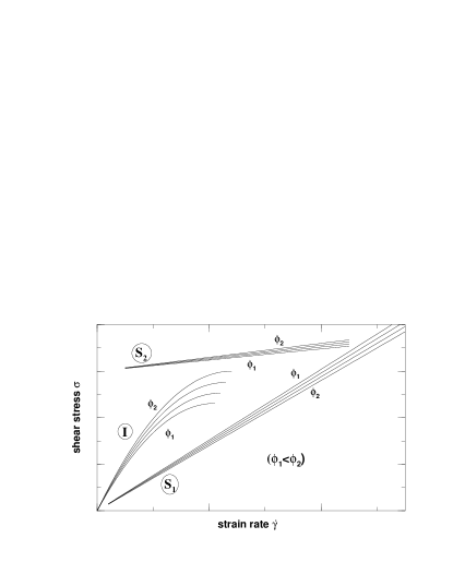
Fig. 1.–: Steady state constitutive curves $\sigma(\dot{\gamma},\phi)$ for a hypothetical fluid with a shear-thinning quiescent state I, a shear-induced phase S₁, and a shear-induced “gel” S₂ with an apparent yield stress. All flow branches have concentration dependences as shown, and are only stable at the points shown.

Despite the surfeit of experiments, theories have been limited to a few systems (micelles [14, 15] and liquid crystals [16, 17, 18, 19]), and few have attempted to calculate an entire phase diagram for a complex fluids solution in flow [19]. In a remarkable paper, Schmitt et al. classified the instabilities that can occur in complex fluid solutions, and clarified the relationship between the nature of the instability (either in primarily the concentration, “spinodal”, or the strain rate, “mechanical”), the shape of the flow curves, and the orientation of the interface that initially develops during the instability [6]. However, as noted in [6], the orientation of an interface in an initial instability may or may not be relevant to the orientation of the macroscopic phase separated state. In this work I outline the different macroscopic phase diagrams that can occur in complex fluid solutions in planar shear flow and describe how phase diagrams determine “flow curves”, the relation between applied shear stress and measured mean strain rate. No attempt is made to pose or solve any specific dynamical models (see [19, 20]), but rather to explore the consequences of possible phase diagrams and provide a phenomenological framework within which to understand the rapidly growing body of rheological experiments.

2 Phenomenology of Phase Coexistence in Shear Flow

Calculations of phase behavior requires first determining the relevant microstructure of the quiescent and flow-induced phases, and deriving equations of motion for the appropriate variables (momentum, mass concentration $\phi$, and variables such as liquid crystalline or crystalline order, or aggregate shape and size distributions). These equations of motion determine the steady state flow curves corresponding to different microstructures. For example, fig. 1 shows a hypothetical shear-thinning fluid I which can be sheared into either a less viscous fluid S₁, or a gel-like state S₂. For this particular fluid the shear-induced phases are stabilized only in finite flow; systems near equilibrium phase transitions such as liquid crystals may have multiple stable flow curves in the limit of zero flow [19], while other systems such as dilute wormlike micelles [7] and “onions” [9, 10, 11] apparently have flow branches which are only stabilized in finite flow. The task of theory, and indeed of experiments, is to understand how material on different flow curves may coexist, and what controls the stability of one phase with respect to another.

At coexistence a fluid partitions into phases with, in principle, different concentrations. In the fluid of fig. 1 the I and S₁ states could coexist at the same shear stress (which would require the interface between phases to lie in the velocity-vorticity plane); as could the S₁ and S₂ states; the I and S₁ phases could not coexist at a common shear stress. Phase coexistence among all three possible pairs of states is conceivable at a common strain rate (requiring an interface lying in the velocity–velocity-gradient plane). Phase diagrams may be constructed by determining the states on distinct stable flow curves for which the driving force for particle exchange vanishes, and for which a mechanically stable stationary interfacial solution between phases can be found. This procedure has been developed for dynamical models which incorporate both smooth [18, 15, 19] and sharp [21, 20] interfaces. In the former case gradient terms are included in the equations of motion, while in the latter case a mechanical condition on interface stability is required. Complete phase diagrams have been calculated for a model system of rigid rod suspensions, for both common stress and common strain rate geometries [19]. Unfortunately, we still lack methods for choosing from several candidate possibilities for phase coexistence.

To begin, consider a complex fluid solution which possesses two distinct phases under shear flow: we denote these I and S (for the example fluid of fig. 1 these could be any of the I, S₁ and S₂ states). We assume this fluid has steady-state macroscopic phase coexistence observed experimentally and hence has a phase diagram which may, in principle, be calculated from the relevant dynamical equations of motion. For simplicity we ignore interesting complications associated with secondary-flow or dynamical instabilities which can induce non-stationary oscillating or chaotic steady states; and ignore any effects of curved geometries.

Given such a fluid, there are two possible geometries for phase coexistence: (A) common stress phase separation, for which phases coexist in the flow gradient direction, and (B) common strain rate phase separation, for which phases coexist in the vorticity direction. For each case, flow can induce a transition to either a less viscous phase (A1, B1) or a more viscous phase (A2, B2). These geometries and flow curves are shown in fig. 2. To understand the concentration dependence of these flow curves we must examine the entire phase diagrams: some possibilities are shown in fig. 3. Upon increasing the concentration the S phase may be stabilized at either weaker flows (A1, B1, A2, etc.) or stronger flows (A1’, B1’, A2’, etc.).

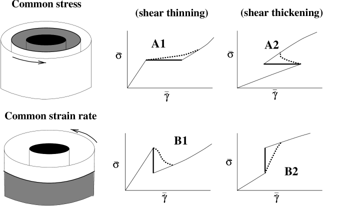
Fig. 2.–: Fundamental rheological signatures for phase separation at common stress (top row, A1 and A2) or common strain rate (bottom row, B1 and B2), for essentially shear thinning (middle, A1 and B1) or shear thickening (right, A2 and B2) transitions. $\bar{\sigma}$ and $\bar{\dot{\gamma}}$ are the imposed (measured) shear stress and strain rate, respectively. The thick solid lines denote the two phase region if $\delta\phi=0$, and the broken lines denote the two-phase region in the event of a finite width biphasic region $|\delta\phi|>0$.

Fig. 3.–: “Fundamental” phase diagrams and flow curves. These have not been calculated, but would be calculated from the homogeneous flow curves (e.g. fig. 1) by the methods of [19] or [21, 20]. The phase boundaries $\dot{\gamma}_{S},\dot{\gamma}_{I},\sigma_{S},\sigma_{I}$ in the top two rows are coincident with the kinks in the flow curves. Top row: shear diagrams in the $\dot{\gamma}\!-\!\phi$ plane. Middle row: shear diagrams in the $\sigma\!-\!\phi$ plane. Thick lines in both planes correspond to the I phase boundary. Bottom row: flow curves $\sigma(\dot{\gamma})$ for representative mean concentrations $\phi_{1}$ and $\phi_{2}$, with thick lines denoting the phase coexistence region; in each case $\phi_{1}$ has a narrower window of coexistence in the relevant control variable plane than does $\phi_{2}$. Tie lines in the $\dot{\gamma}\!-\!\phi$ plane move to higher strain rates with increasing stress. A1 and A2: phase separation at common stress with the S phase stabilized at a lower stress for increasing concentration. A1’ and A2’: phase separation at a common stress, with S phase stabilized at a higher stress for increasing concentration. B1 and B2 phase separation at a common strain rate.

3 Common Stress Phase Separation

We first consider coexistence at a common stress (A1, A2, A1’, A2’), for which the mean strain rate $\bar{\dot{\gamma}}$ and mean concentration $\bar{\phi}$ at stress $\sigma$ are partitioned according to

$$\bar{\dot{\gamma}} = \alpha\,{\dot{\gamma}}_{I}(\phi_{I})+(1-\alpha)\,\dot{\gamma}_{S}(\phi_{S}),$$ (1)

$$\bar{\phi} = \alpha\,{\phi}_{I}+(1-\alpha)\,\phi_{S},$$ (2)

with $\alpha$ the fraction of material in the I phase. Phase coexistence occurs in a region in the $\sigma\!-\!\phi$ plane, with horizontal tie lines connecting the coexisting points $(\phi_{I},\dot{\gamma}_{I})$ and $(\phi_{S},\dot{\gamma}_{S})$. This may also be represented in the $\dot{\gamma}\!-\!\phi$ plane. The lines $\{\phi_{I}(\sigma),\phi_{S}(\sigma),\dot{\gamma}_{I}(\phi_{I}(\sigma)),\dot{\gamma}_{S}(\phi_{S}(\sigma))\}$ bound the phase coexistence regions. The slope of tie lines in the $\dot{\gamma}\!-\!\phi$ plane reflects the compositions of the two phases; vertical tie lines imply equal concentrations, while a non-infinite slope implies different concentrations. The flow curves $\sigma({\dot{\gamma}},\bar{\phi})$ can be calculated from the phase diagrams and eqs. 1 and 2 by applying the lever rule. They are non-analytic at the stresses and strain rates which bound the biphasic region, and would be obtained in experiment at a given mean concentration $\bar{\phi}$. In the biphasic region the stress increases by crossing successive tie lines in the $\dot{\gamma}\!-\!\phi$ plane, and varies according to the tie line spacing and splay [19]. From eqs. 1 and 2 one can calculate the shape of the stress “plateau” [6]:

$$\left.\frac{d\sigma}{d{\bar{\dot{\gamma}}}}\right|_{\bar{\phi}}=\left[\frac{\alpha}{\eta_{I}}+\frac{1-\alpha}{\eta_{S}}-m(\sigma,\bar{\phi})\left\{\frac{1-\alpha}{\dot{\gamma}^{\prime}_{S}\eta_{S}}+\frac{\alpha}{\dot{\gamma}^{\prime}_{I}\eta_{I}}\right\}\right]^{-1},$$ (3)

where $m(\sigma,\bar{\phi})$ is the slope of the tie line, $\eta_{k}=\partial\sigma/\partial{\dot{\gamma}}$ is the local viscosity of the $k$th branch, and $\dot{\gamma}^{\prime}_{k}=\partial\dot{\gamma}_{k}/\partial\phi$. Experiments on worm-like micelles have revealed that some systems can be “superstressed” to a metastable state, with the stress entering the biphasic region [4, 2, 22].

For an A1 (or A1’) shear-thinning transition the strain rate increases as the stress is increased through the two phase region. The stress through the two-phase region increases less for mean concentrations $\bar{\phi}$ for which the biphasic window is narrow (e.g. $\phi_{1}$) or the tie lines are steep in the $\dot{\gamma}\!-\!\phi$ planel, and deviates more from constant for a wider biphasic region (e.g. $\bar{\phi}=\phi_{2}$) with more vertical tie lines. Hence, a signature of substantial concentration difference $\delta\phi\equiv\phi_{I}-\phi_{S}$ between coexisting phases is a large increase in stress through the biphasic region. This is consistent with calculations on a model for rigid rods in shear flow [19], and measurements on shear-thinning wormlike micelles [1, 2, 3, 4, 5, 6]. In dilute micelles $\delta\phi$ is typically negligible and the stress plateau is nearly flat; while $\delta\phi$ increases for concentrated solutions near an underlying isotropic-nematic transition and the stress plateau acquires a shape.

For the A1 fluid the S phase can have a larger ($m(\sigma,\bar{\phi})>0$) or smaller ($m(\sigma,\bar{\phi})<0$) strain rate than the I phase. In the latter case the S phase has a larger effective viscosity, and for a small enough $\delta\phi$ the fluid crosses over to a characteristic shear-thickening fluid, A2. In this case the strain rate actually decreases as the stress is increased through the two phase region. That is, the system remains in the I phase below a critical strain rate at which a band of more viscous material S develops whose small strain rate reduces the measured strain rate. Hence the system enters the biphasic region in the $\dot{\gamma}\!-\!\phi$ plane at the high strain rate, and traverses from top to bottom. Upon increasing the stress the system converts into the S phase with, in general, changing I and S concentrations, until the I phase disappears at the lower boundary of the two-phase envelope in the $\dot{\gamma}\!-\!\phi$ plane. For higher stresses the system follows the constitutive branch for the S phase and traces a vertical path in the $\dot{\gamma}\!-\!\phi$ plane. Hence the flow curve $\sigma({\dot{\gamma}})$ has a distinct S shape. As with flow A1, the shape of the flow curve in the biphasic region depends on the slope of the tie lines (i.e. $\delta\phi$) in the $\dot{\gamma}\!-\!\phi$ plane: vertical tie lines $\delta\phi=0$ imply a vertical jump in $\sigma(\dot{\gamma})$, while finite $\delta\phi$ and flatter tie lines imply a gentler slope for $\sigma({\dot{\gamma}})$. Flow A2’ has been seen in shear-thickening wormlike micelles [7], and calculated using a phenomenological model [20]. Flow A2 (or A2’) has been seen in surfactant onion crystals under shear, although the band geometry has not been verified [10].

We have drawn (A1,A2,A1’,A2’) with finite biphasic regions at zero stress, corresponding to a perturbation of an existing phase transition. However, fluids such as the example fluid in fig. 1 would have phase coexistence only above a finite stress. The construction of these phase diagrams implies that tie lines move to higher strain rates with increasing stress (“conventional”). Although intuitive, the reverse (“unconventional”) does not violate any physical laws. For example, a version of A2’ with unconventional positive-sloped tie lines, would imply a $\sigma\!-\!\phi$ biphasic region moving to smaller $\phi$ with increasing $\sigma$. However, a version of A2’ with negative-sloped tie lines yields a nonsensical phase diagram.

4 Common Strain Rate Phase Separation

For coexistence at a common strain rate the shear stress is partitioned according to

$$\bar{\sigma}=\alpha\,{\sigma}_{I}(\phi_{I})+(1-\alpha)\,\sigma_{S}(\phi_{S}),$$ (4)

and the two main classes of flows are shown as B1 and B2. We do not show analogous diagrams B1’ and B2’, for which the coexistence strain rate increases with increasing concentration. For flow B2 the stress increases through the two phase region and the transition is to either a thicker or (for large enough $\delta\phi$, as with flow A1) thinner phase. The shape of the stress through the two phase region is given, from eqs. 2 and 4

$$\left.\frac{d\bar{\sigma}}{d{\dot{\gamma}}}\right|_{\bar{\phi}}=\eta_{I}\,\alpha+\eta_{S}\,(1-\alpha)-m(\dot{\gamma},\bar{\phi})\left\{\frac{\eta_{S}(1-\alpha)}{\sigma^{\prime}_{S}}+\frac{\eta_{I}\,\alpha}{\sigma^{\prime}_{I}}\right\},$$ (5)

where $m(\dot{\gamma},\bar{\phi})$ is the slope of the tie line and $\sigma^{\prime}_{k}=\partial\sigma_{k}/\partial\phi$. In the limit of no concentration difference ($\delta\phi=0$ or $m(\dot{\gamma},\bar{\phi})=\infty$), $\sigma(\dot{\gamma})$ is vertical through the two phase region. Flow B1 is a shear thinning transition, and the stress decreases through the two-phase region. Banding geometries and flow curves similar to B1 were reported in an onion system [11], although this may not have been steady state. B2 has been reported in an onion system [9].

5 Applications

The shear diagrams presented do not exhaust the possibilities; these flow behaviors can be combined smoothly in many ways. We present two possibilities in fig. 4. Fluid C1 phase separates at a common stress, and $\delta\phi$ widens with increasing concentration, crossing over from shear thickening (A2) to shear thinning (A1) as the concentration increases. Fluid C2 phase separates at a common strain rate, with a coexistence width $\delta\phi$ that narrows with increasing $\phi$, combining B1’ and B2’ behavior.

Fig. 4.–: More complex possibilities for phase separation at common stress (C1: top row) or common strain rate (C2: bottom row). $\phi_{1},\phi_{2}$, and $\phi_{3}$ are representative mean concentrations.

Typical experiments extract a series of steady state flow curves for different concentrations $\{\phi_{i}\}$. Consider coexistence at common stress. The flow curves have kinks at the boundaries of the biphasic region, $\{(\sigma_{Ii},\dot{\gamma}_{Ii},\phi_{i})\}$ and $\{(\sigma_{Si},\dot{\gamma}_{Si},\phi_{i})\}$, which should be corroborated optically or otherwise. The strain rates and concentrations of the coexisting states may be determined as follows. One first fits curves $\sigma_{I}(\phi),\sigma_{S}(\phi),\dot{\gamma}_{I}(\phi),\dot{\gamma}_{S}(\phi)$ to the values extracted from the kinks. A horizontal tie line connecting $(\phi_{I},\phi_{S})$ at a given stress $\sigma_{\ast}$ may then be read off the biphasic boundaries, $\sigma_{I}(\phi_{I\ast})=\sigma_{S}(\phi_{S\ast})=\sigma_{\ast}$ in the $\sigma\!-\!\phi$ plane; and the corresponding tie lines on the $\dot{\gamma}\!-\!\phi$ plane connects the points $\dot{\gamma}_{I}(\phi_{I\ast})$ and $\dot{\gamma}_{S}(\phi_{S\ast})$. In this way the complete shear diagrams and characteristics of coexisting states, may be constructed. As a check, the shape of $\sigma({\dot{\gamma}})$ through the two-phase region may be computed by traversing the biphasic regions of the $\dot{\gamma}\!-\!\phi$ and $\sigma\!-\!\phi$ planes and using the lever rule to construct the mean strain rate via eq. (1). This analysis is necessary if the coexisting concentrations cannot be determined directly and, in the two phase region, the flow curve has a slope appreciably different from zero (common stress phase separation) or infinity (common strain rate phase separation).

Returning to the hypothetical fluid of fig. 1, we expect common stress phase separations I-S₁ and S₁-S₂ to be classes A1 and A2 (or A1’ and A2’), respectively, with the former disappearing at higher stresses; and common strain rate phase separations I-S₁, I-S₂, and S₁-S₂ to be classes B1, B2, and B2 (or B1’, B2’, B2’), respectively. Since flow is necessary to stabilize the S₁ and S₂ phases, the biphasic window in this system would appear at a finite stress or strain rate. Note that the accessibility and even stability of composite flow curves depends on the control variable of the rheometer. For example, composite flow curves with negative slope $d{\sigma}/d{\dot{\gamma}}<0$ (e.g. A2 and B1) could be mechanically unstable [6], although ref. [7] accessed such a curve under controlled stress conditions. Finally, kinetic possibilities such as metastability and hysteresis are sure to enrich the relatively simple scenarios proposed above.

***

It is a pleasure to thank David Lu, Armand Ajdari, Ovidiu Radulescu, Jacqueline Goveas, and Tom McLeish for encouragement and enjoyable discussions.

References

- [1] Rehage, H. and Hoffmann, H., Mol. Phys., 74 (1991) 933.
- [2] Berret, J. F., Roux, D. C., and Porte, G., J. Phys. II (France), 4 (1994) 1261.
- [3] Cappelaere, E., Berret, J. F., Decruppe, J. P., Cressely, R., and Lindner, P., Phys. Rev. E, 56 (1997) 1869.
- [4] Grand, C., Arrault, J., and Cates, M. E., J. Phys. II (France), 7 (1997) 1071.
- [5] Britton, M. M. and Callaghan, P. T., Phys. Rev. Lett., 78 (1997) 4930; Mair, R. W. and Callaghan, P. T., J. Rheol., 41 (1997) 901.
- [6] Schmitt, V., Marques, C. M., and Lequeux, F., Phys. Rev., E52 (1995) 4009.
- [7] Liu, C. H. and Pine, D. J.,Phys. Rev. Lett., 77 (1996) 2121-2124; Boltenhagen, P., Hu, Y. T., Matthys, E. F., and Pine, D. J., Phys. Rev. Lett., 79 (1997) 2359; Hu, Y. T., Boltenhagen, P., and Pine, D. J., J. Rheol., 42 (1998) 1185.
- [8] Noirez, L. and Lapp, A., Phys. Rev. Lett., 78 (1997) 70.
- [9] Diat, O., Roux, D., and Nallet, F., J. Phys. II (France), 3 (1993) 1427; Phys. Rev., E (1995) 3296.
- [10] Sierro, P. and Roux, D., Phys. Rev. Lett., 78 (1997) 1496.
- [11] Bonn, D., Meunier, J., Greffier, O., Alkahwaji, A., and Kellay, H., Phys. Rev. E, 58 (1998) 2115.
- [12] Safinya, C. R., Sirota, E. B., and Plano, R. J., Phys. Rev. Lett., 66 (1991) 1986.
- [13] Mather, P. T., Romo-Uribe, A., Han, C. D., and Kim, S. S., Macromolecules, 30 (1997) 7977.
- [14] Cates, M. E. and Turner, M. S., J. Phys. Cond. Matt., 4 (1992) 3719; Bruinsma, R., Gelbart, W. M., and Benshaul, A., J. Chem. Phys., 96 (1992) 7710.
- [15] Spenley, N. A., Yuan, X. F., and Cates, M. E., J. Phys. II (France), 6 (1996) 551.
- [16] Hess, S., Naturforsch., 31a (1976) 1507.
- [17] Bruinsma, R. F. and Safinya, C. R., Phys. Rev., E43 (1991) 5377.
- [18] Olmsted, P. D. and Goldbart, P. M., Phys. Rev., A41 (1990) 4578; Phys. Rev., A46 (1992) 4966.
- [19] Olmsted, P. D. and Lu, C.-Y. D., Phys. Rev., E56 (1997) 55; Phys. Rev. E (1999) (in press).
- [20] Goveas, J. L. and Pine, D. J., Europhys. Lett. (submitted), (1999) .
- [21] Ajdari, A., Phys. Rev., E58 (1998) 6294.
- [22] Berret, J. F., Langmuir, 13 (1997) 2227.
- [23] Porte, G., Berret, J. F., and Harden, J. L., J. Phys. II (France), 7 (1997) 459.