Interaction Round a Face DMRG method
applied to rotational invariant quantum spin chains

Abstract

An interaction-round-a-face density-matrix renormalization-group (IRF-DMRG) method is developed for higher integer spin chain models which are rotational invariant. The expressions of the IRF weights associated with the nearest-neighbor spin-$S$ interaction ${\bf S}_{i}\cdot{\bf S}_{i+1}$ are explicitly derived. Using the IRF-DMRG with these IRF weights, the Haldane gaps $\Delta$ and the ground state energy densities $e_{0}$ for both $S=1$ and $S=2$ isotropic antiferromagnetic Heisenberg quantum spin chains are calculated by keeping up to only $m=90$ states.

]

I Introduction

Density matrix renormalization group (DMRG) method has been a powerful numerical tool since White’s pioneering works [1]. DMRG is a real space numerical renormalization method by using the reduced density matrix of a large system to approximate the ground (or excited) state(s) of the system with great accuracy. There are many DMRG applications for (quasi)one-dimensional (1D) systems, e.g., quantum systems, statistical systems, polymers, etc.(for a review see Ref. [2], and references therein).

DMRG is also a variational method and closely related to matrix product (MP) method [3, 4, 5, 6]. In MP method the ground state of a system, which is assumed to be expressed as a matrix product, can be obtained by minimizing the associated ground state energy density with respect to variational parameters. On the other hand DMRG method may find the ground state of a large system, which consists of Wilsonian blocks, $B^{L}\bullet\bullet B^{R}$, by keeping the most probable $m$ states for each block $B^{L/R}$. The most $m$ probable states are selected by using the $m$-largest eigenvalues of the reduced density matrix $\rho^{L/R}$ for each block. For an overview and some connections to related fields including MP method, Ref. [6] is recommended.

When a system of interest has a symmetry, the associated eigenvalues of the density matrix $\rho$ are degenerated and one should keep the all states that corresponding to the same eigenvalues. For example, if we consider a rotational invariant model, e.g., 1D isotropic Heisenberg spin models, with the standard vertex-DMRG, we may use third components $s_{z}$ of spin as basis, then the eigenvalues of the density matrix are degenerated due to the rotational symmetry. One thus needs to keep many states to improve numerical accuracy with $s_{z}$ basis in order to get a real physics at thermodynamic limit. There have been large-scale DMRG calculations with many states kept, for example, up to $m=300$ [7], $m=400$ [8], $m=1700$ [9], to estimate the $S=2$ Haldane gap. However the more $m$ states are kept, the more computational cost is necessary since the dimension of the Hilbert space for the superblock $B^{L}\bullet\bullet B^{R}$ is proportional to $m^{2}$.

Sierra and Nishino[10] had applied the DMRG method to interaction round a face (IRF) models and developed the IRF-DMRG method. The advantage of using IRF-DMRG method in a system which has rotational symmetry is that the dimensions of the associated Hilbert spaces are much smaller than that in standard vertex-DMRG, since the degeneracy due to the symmetry has been eliminated. They had demonstrated the power of the IRF-DMRG by calculating the ground state energies of the solid on solid (SOS) model, which is equivalent to spin-$1/2$ Heisenberg chain, and that of the restricted SOS (RSOS) model, which is equivalent to the quantum group invariant XXZ chain. They also had suggested a promising potential of the IRF-DMRG when it applies to higher integer quantum spin chains. Such a work has not yet been done as far as I know.

In this work, the IRF-DMRG method is reviewed and further developed for the 1D integer spin antiferromagnetic Heisenberg (AFH) quantum spin chains. In IRF formulation the dynamics of a model can be described by a local plaquette operator $X_{i}$, which operates to the $i$th site of an IRF state as a “diagonal to diagonal transfer matrix” and their matrix elements are called the IRF weights as will be explained in the next section. We hence need the explicit expressions of the IRF weights for the higher integer quantum spin chain models in order to work with the IRF-DMRG.

The rest of the paper is organized as follows. In the next section the IRF-DMRG method is reviewed. After the explanation of IRF formulation, the infinite system algorithm of the IRF-DMRG is discussed. How to target the excited states of AFH quantum spin chains are explained and the superblock configuration suited for targeting the excited state of the AFH spin chain is proposed. In Sec. III, the power of the IRF-DMRG is demonstrated by applying it to both $S=1$ and $S=2$ AFH quantum spin chains. The Haldane gaps are calculated by keeping moderate number of $m$ states. Finally conclusions are stated. With the help of the Wigner Ekart’s theorem summarized in Appendix A, I’ve derived the expression of the IRF weights for a nearest neighbor spin-$S$ interaction ${\bf S}_{i}\cdot{\bf S}_{i+1}$ in Appendix B. These expressions enable us to work with the IRF-DMRG.

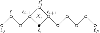
FIG. 1.: Diagrammatic representation of the operation of a plaquette operator $X_{i}$ on a IRF state $|\ell_{0},\cdots,\ell_{i},\cdots,\ell_{N}\rangle$, which is drawn as a zigzag chain of the lattice sites (open circles). The closed circle stands for the summation over the lattice variable $\ell_{i}$.

II Review of IRF-DMRG

The IRF-DMRG method is briefly reviewed here according to the Sierra and Nishino’s paper [10]. It is instructive to begin with a brief review of graph IRF model in somewhat general context. The IRF representation of a rotational invariant quantum spin chain is then explained with the help of the associated spin graphs. In fact 1D quantum spin chain models can be formulated as a special case of graph IRF models. The algorithm of the IRF-DMRG is also reviewed. A method how to target the excited states of AFH quantum spin chains and the appropriate superblock configurations are explained.

A Graph IRF model

In interaction round a face or face models for short [11, 12], a state is represented with the lattice variables $\ell$ assigned to the lattice sites;

$$|{\bf\ell}\rangle=|\ell_{0},\ell_{1},\ldots,\ell_{N}\rangle,$$ (1)

while the associated interaction is defined on a face, or plaquette of the lattice sites;

$$X_{i}|\dots,\ell_{i-1},\ell^{\prime}_{i},\ell_{i+1},\dots\rangle\hskip 72.26999pt$$ (2)

$$=\sum_{\ell_{i}}R\left(\begin{array}[]{ccc}&\ell^{\prime}_{i}&\\ \ell_{i-1}&&\ell_{i+1}\\ &\ell_{i}&\\ \end{array}\right)|\dots,\ell_{i-1},\ell_{i},\ell_{i+1},\dots\rangle,$$ (6)

where $R$ are so called IRF weights, which play an important role such as Boltzmann weights in usual statistical models. The dynamics of the model is described by a plaquette operator $X_{i}$, which consists of the associated IRF weights. The plaquette operator $X_{i}$ can be viewed as a local “diagonal transfer matrix” as shown in Fig. 1 in contrast with a usual “row to row transfer matrix.”

IRF model is characterized with a selection rule which determines whether the adjacent lattice sites of a lattice site are admissible or not. The selection rule can be described by its associated incident matrix $\Lambda_{\ell,\ell^{\prime}}$, whose elements are all either $0$ or $1$. If $\Lambda_{\ell,\ell^{\prime}}=0$, then the lattice variables $\ell$ and $\ell^{\prime}$ cannot be assigned to adjacent lattice sites, i.e., not admissible to each other. The $\Lambda$ characterizes the set of all possible configurations which contribute to the Hamiltonian or partition function of the IRF model. A configuration not derived from $\Lambda$ necessarily has zero IRF weight. It may be more convenient to use a graph or diagram associated with the selection rule, or $\Lambda$, of an IRF model and this is called a graph IRF (or graph face) model. Each vertex of such a graph represents a lattice site $\ell_{i}$, which may take values from $1$ to $n_{i}$, and they are connected with line if they are admissible.

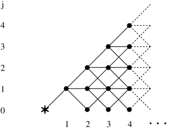
FIG. 2.: Spin diagram for $S=1$ chain. Each vertex represents an IRF lattice site. The height of each site represents the total spin angular momentum $j_{i}$ summing from the most left vertex $\ast$ (vacuum state) until the $i$th spin. Admissible vertices are connected with lines.

For a rotational invariant spin chain, the corresponding selection rule is nothing but the addition rule of spin angular momenta, each spin state is hence classified with the total spin angular momentum $j$. The states of the chain with $N$ spins will be given by the set $|j_{N},M\rangle$ ($j^{\rm min}\leq j_{N}\leq j^{\rm max}$) of states with total spin $j_{N}$ and the corresponding third component $M$. One of the graphical representations associated with the addition rule of spin is the so called spin diagram. For example, the spin diagram for $S=1$ spin chain is shown in Fig. 2. The corresponding lattice variables $\ell_{i}$ of the spin diagram are the magnitudes $j_{i}$ of spin angular momenta until the $i$th spin. The height of each vertex represents the sum $j_{i}$ of the spin angular momenta starting from the most left spin until the $i$th spin. The $i$th and ($i+1$)-th vertices are connected if they are admissible, i.e., if they are satisfied with the addition rule; $|j_{i}-S|\leq j_{i+1}\leq j_{i}+S$, where $S=1$ for spin-$1$ chain. Note that $j_{i}$ takes values from $j_{i}^{\rm min}$ to $j_{i}^{\rm max}$, i.e., the range of $j_{i}$ is site dependent. An IRF state of the $N$ spin chain is represented by a path in the spin diagram $|\ast,j_{1},j_{2},\cdots,j_{i},\cdots,j_{N}\rangle$ and the most left vertex $\ast$ is corresponding to a vacuum state $|0\rangle$. If we know the all IRF weights associated with a spin chain model, we can work in the IRF formulation. It is hence important to derive the explicit expressions for the IRF weights of the spin chain model to apply the IRF-DMRG. In Appendix B, I have derived the expression of the IRF weights for the nearest neighbor spin-$S$ interaction and summarized the diagrammatic representations and the corresponding IRF weights as a function of spin $j$ for the $S=1$ isotropic AFH case in Fig. 12.

B Algorithm

The DMRG is an iterative algorithm to approximate a target state (the ground or excited state) of a large system which consists of the two blocks and lattice site(s). In each iteration each block is extended by adding one lattice site but keeping only the most $m$ probable states, which are selected with the density matrix constructed from the target state. The superblock[15] is formed by the left block $B^{L}$, the middle block which consists of a lattice point $\bullet$ or of two points $\bullet\bullet$, and the right block $B^{R}$, which is not necessarily the reflection of $B^{L}$.

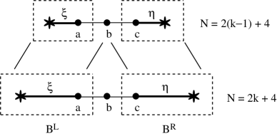
FIG. 3.: Schematic diagram of the infinite IRF-DMRG algorithm. Each block (dotted line box) is extended by adding single middle lattice point $\bullet$ in each DMRG iteration. Thick lines represent renormalized block states.

Let me first review the infinite system algorithm [10] of the IRF-DMRG. A Hilbert space of the superblock $B^{L}\bullet B^{R}$ can be written as

$${\mathcal{H}}^{B^{L}\bullet B^{R}}=\{|\xi_{a}\otimes b\otimes\eta_{c}\rangle\quad|\quad\Lambda_{a,b}=\Lambda_{b,c}=1\},$$ (7)

i.e., a space spanned by a left block state $|\xi_{a}\rangle$, a middle lattice point state $|b\rangle$, and a right block state $|\eta_{c}\rangle$ (see Fig. 3), where the three lattice points (a, b, c) must be connected in a associated spin diagram. These lattice points take values from $j_{i}^{\rm min}$ to $j_{i}^{\rm max}$, where $i=a,b,c$.

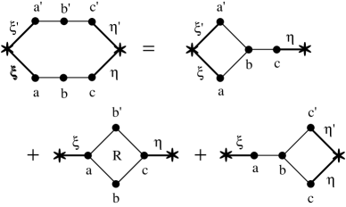
FIG. 4.: Diagrammatic representation for the construction of the super block Hamiltonian $H^{B_{L}\bullet B_{R}}$; each diagram is corresponding to each term in Eq. (21).

The superblock Hamiltonian $H^{B^{L}\bullet B^{R}}$ can be constructed from the two block Hamiltonians $H^{B^{L}}$, $H^{B^{R}}$ and the IRF weights $R$ using the following relation,

$$H_{\xi_{a},b,\eta_{c}}^{\xi^{\prime}_{a},b^{\prime},\eta^{\prime}_{c}}\left(\begin{array}[]{lllll}&a^{\prime}&b^{\prime}&c^{\prime}&\\ \ast&&&&\ast\\ &a&b&c&\end{array}\right)=H_{\xi_{a}}^{\xi^{\prime}_{a}}\left(\begin{array}[]{lll}&a^{\prime}&\\ \ast&&b\\ &a&\end{array}\right)\delta_{b}^{b^{\prime}}\Lambda_{b,c}\delta_{\eta_{c}}^{\eta^{\prime}_{c}}$$ (14)

$$+\delta_{\xi_{a}}^{\xi^{\prime}_{a}}R\left(\begin{array}[]{lll}&b^{\prime}&\\ a&&c\\ &b&\end{array}\right)\delta_{\eta_{c}}^{\eta^{\prime}_{c}}+\delta_{\xi_{a}}^{\xi^{\prime}_{a}}\delta_{b}^{b^{\prime}}\Lambda_{a,b}H_{\eta_{c}}^{\eta^{\prime}_{c}}\left(\begin{array}[]{lll}&c^{\prime}&\\ b&&\ast\\ &c&\end{array}\right).$$ (21)

Figure 4 shows the diagrammatic representation of the above equation.

We then may find the ground (or excited) state of the superblock by using a Lanczos or similar method,

$$|\Psi_{G}\rangle=\sum_{\xi_{a},b,\eta_{c}}\psi^{b}_{\xi_{a},\eta_{c}}|\xi_{a}\otimes b\otimes\eta_{c}\rangle.$$ (22)

The left density matrix $\rho^{B^{L}\bullet}$ is readily constructed as

$$\rho^{\xi^{\prime}_{a}}_{\xi_{a}}\left(\begin{array}[]{lll}&a^{\prime}&\\ \ast&&b\\ &a&\\ \end{array}\right)=\sum_{\eta_{c}}\psi^{b}_{\xi^{\prime}_{a},\eta_{c}}\psi^{b}_{\xi_{a},\eta_{c}}.$$ (23)

The right density matrix $\rho^{B^{R}\bullet}$ is constructed in the similar way if necessary.

The next step is to diagonalize $\rho^{B^{L}\bullet}$ to obtain the eigenvalues $w^{b}$ and the associated eigenvectors $|u^{b}_{\xi_{a}}\rangle$. Keeping the $m$ states associated with $m$-largest $w^{b}$ ($m=\sum_{b}m_{b}$) in order to form the projection operator $T^{{\dagger}}T$.

$$T=\sum_{b}T^{b},\hskip 28.45274ptT^{b}=\sum_{\xi_{a}}|u^{b}_{\xi_{a}}\rangle\langle u^{b}_{\xi_{a}}|$$ (24)

The operator $T$ truncates the Hilbert space ${\mathcal{H}}^{B^{L}\bullet}$ into ${\mathcal{H}}^{B^{\prime L}}$, where $B^{\prime L}$ represents a block with one more lattice site than the block $B^{L}$. A new left block Hamiltonian is then formed by using the projection operator as $H^{B^{\prime L}}=T(H^{B^{L}\bullet})T^{{\dagger}}$. In each IRF-DMRG iteration the system is extended by adding single middle site $\bullet$ to both blocks as shown in Fig. 3.

The infinite system algorithm for the IRF-DMRG with the superblock $B^{L}\bullet B^{R}$ is summarized as follows:

1. find the ground state of the superblock Hamiltonian, Eq. (21);

2. form the left (right) reduced density matrix $\rho^{B^{L}\bullet}$ ($\rho^{B^{R}\bullet}$), Eq. (23);

3. diagonalize $\rho^{B^{L}\bullet}$ ($\rho^{B^{R}\bullet}$) to obtain the eigenvalues $w^{b}$ and the associated eigenvectors $|u^{b}_{\xi_{a}}\rangle$ ( $|u^{b}_{\eta_{c}}\rangle$);

4. keep the $m$ states $|u^{b}_{\xi_{a}}\rangle$ corresponding to the $m$ largest eigenvectors $w^{b}$ to form the projection operator $T$, Eq. (24);

5. renormalize the block operators by using $T$:
   $H^{B^{\prime L}}=T(H^{B^{L}\bullet})T^{{\dagger}}$, etc.;

6. extend each block by adding one site $\bullet$;

repeat the processes i)-vi) for new blocks.

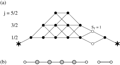
FIG. 5.: (a) Spin diagram of the superblock for targeting the excited state or the ground state of the $S=1$ open spin chain ended with $S=1/2$ spins. (b) The corresponding spin chain of $N=4$ spin-$1$ spins (large hatched circles) ended with spin-$1/2$ spins (small open circles). For targeting the excited states, which has total spin $S^{T}=1$, ferromagnetic coupled two spin-$1/2$ spins are attached.

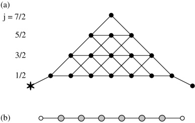
FIG. 6.: (a) Spin diagram of $S=1$ chain ended with $S=1/2$ spins. AKLT state is corresponding to the horizontal line at $j=1/2$. (b) The corresponding spin chain of $N=6$ spin-$1$ spins (large hatched circles) ended with spin-$1/2$ spins (small open circles).

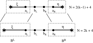
FIG. 7.: Schematic diagram of the proposed infinite IRF-DMRG algorithm. The left (right) block is extended by adding single middle left (right) point $\bullet$ in each IRF-DMRG iteration

Next let me explain how to target the excited state of the AFH spin chain before discussing the superblock configuration suited for the excited state. Figure 5 shows how to target the excited state of the AFH spin-$1$ spin chain ended with spin-$1/2$ spins. In order to fix the total spin $S_{T}$ of the chain in $S_{T}=1$ sector, two spin-$1/2$ spins that ferromagnetically coupled with the coupling constant $J_{F}<0$ are attached as shown in Fig. 5 (b). Note that the attached two spins, which energetically favor a triplet state, are not coupled with the chains. Since the whole system (the chain and the two spins) is set to a singlet state ($0$ sector), the triplet state of the two spins enforce $S_{T}=1$ on the chain [13].

Now let us consider the superblock configuration that suited for targeting the excited state. In the infinite system algorithm of the IRF-DMRG with the superblock configuration of $B^{L}\bullet B^{R}$, the middle point is single bare site and plays an important role to successively improve the renormalized block Hamiltonians. In each IRF-DMRG iteration both blocks are renormalized with the middle site as shown in Fig. 3. In Ref. [10] the superblock configuration of $B^{L}\bullet B^{R}$ was used and it is suited for targeting the ground states of AFH spin chains, because the highest $j$ site always lies in the middle of the superblock as shown in Fig. 6. Since the ground state of an AFH quantum spin chain with even $N$ spins lies in the total spin $0$ sector, $j_{N}=0$ and obviously the vacuum state $\ast$ has zero spin, i.e., $j_{0}=0$. Furthermore the system is reflection symmetric with respect to the middle point in the spin diagram. Thus the middle point always has the highest $j$ in the IRF-DMRG formulation when targeting the ground state of the AFH spin chain. In other word the highest $j$ of the left block, which is constructed from the left vacuum by adding spins, coincides with that of the right block, which is constructed from the right vacuum, at the middle point in the spin graph.

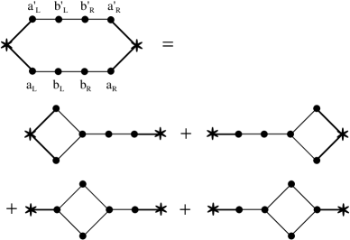
FIG. 8.: Diagrammatic representation for the construction of the super block Hamiltonian $H^{B_{L}\bullet\bullet B_{R}}$.

However the situation is somewhat different for targeting the excited state which lies in $S_{T}=1$ sector. From Fig. 5 (a), we noticed that no single middle point at which the highest $j$ of the left block coincides with that of the right one and that there is no reflection symmetry. Hence it is better to use the superblock configuration of $B^{L}\bullet\bullet B^{R}$, at least when we use the infinite system method, and renormalize $B^{L}$ ($B^{R}$) with the middle left (right) site individually as shown in Fig. 7. The associated superblock Hamiltonian can be constructed in the way diagrammatically shown in Fig. 8.

III Application to $S=1$ and $S=2$ antiferromagnetic Heisenberg quantum spin chains

The supremity of the IRF-DMRG method is demonstrated by applying to both $S=1$ and $S=2$ quantum spin chains. Haldane’s conjecture [14] that the physics of isotropic antiferromagnetic quantum spin chains depend substantially on whether the spin is integer or half-integer, has been motivating many physicists to study quantum spin chains. $S=1$ AFH chain have been widely studied with various methods [16]. It is a well known fact that the ground state of an open $S=1$ quantum spin chain has an effective $S=1/2$ spin at each end. White [17] had obtained the ground state energy per site of $e_{0}\cong-1.401484038971(4)$ with $m=180$ states kept and the Haldane gap of $\Delta_{1}\cong 0.41050(2)$ with $m=160$ states kept by using the standard $s_{z}$-base DMRG.

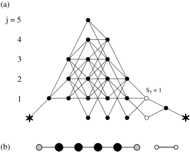
FIG. 9.: (a) Spin diagram of open $S=2$ spin chain ended with $S=1$ spins. The total $S^{T}=1$ state is targeted to find the excited state. (b) The corresponding spin chain of $N=4$ spin-$2$ spins (large closed circles) ended with spin-$1$ spins (hatched circles). The attached two spin-$1/2$ spins (small open circles) are coupled ferromagnetic or antiferromagnetic depending on the target state.

$S=2$ AFH quantum spin chains have also been studied [7, 8], although the numerical calculations are much elaborative than that of $S=1$ case due to the longer correlation length $\xi$ and due to the larger number of degrees of freedom per spin because the degeneracy due to the spin symmetry. The longer correlation length means that much longer chains (more than one thousand) are required to reach the convergence regime to exclude the finite size effects. Schollwöck et al.[7] estimated that the gap of $\Delta_{2}\cong 0.085(5)$ and the ground state energy density to be $e_{0}\cong-4.761248(1)$ by using the standard DMRG with up to $m=210$ states kept. Wang et al. [8] systematically analyzed and estimated that the gap $\Delta_{2}\cong 0.0876\pm 0.0013$ with up to $m=400$ states kept during DMRG calculations.

Following Schollwöck et al., I also consider the open spin-$S$ AFH quantum spin chain terminated with spin-$S/2$ spins to cancel out the effective spin-$S/2$ spins:

$$H=J_{\rm end}{\bf S}_{1}\cdot{\bf S}_{2}+J\sum_{i=2}^{N-2}{\bf S}_{i}\cdot{\bf S}_{i+1}+J_{\rm end}{\bf S}_{N-1}\cdot{\bf S}_{N},$$ (25)

where the both coupling constants $J$ and $J_{\rm end}$ are set to unity for simplicity. The spin diagram for the $S=1$ ground state is shown in Fig. 6. I have obtained the comparable result of $e_{0}\cong-1.40148403897$ with the IRF-DMRG by keeping only $m=80$ states, which consist of $25(j=1/2)$, $31(j=3/2)$, $19(j=5/2)$, and $5(j=7/2)$ $m_{j}$ states, without resorting to a scaling technique. Note that since $m_{j}$ states in $j$ base correspond to $(2j+1)m_{j}$ in $s_{z}$ base, the above $m=80$ correspond to $m=328$ in $s_{z}$ base. For the $S=2$ chain with $N\approx 200$, I have found that the ground state energy density is $e_{0}\cong-4.7612481(6)$ by keeping $m=90$ states, which consist of $9(j=0)$, $24(j=1)$, $27(j=2)$, $19(j=3)$, $9(j=4)$, and $2(j=5)$ $m_{j}$ states, hence corresponding to $m=452$ states in $s_{z}$ base.

The finite size correction to the Haldane gap $\Delta_{S}$ with open boundary conditions is proportional to the inverse of the square chain length according to the 1D field theory [18, 19]:

$$\Delta(m=\infty,N)=\Delta_{S}+\frac{v^{2}\pi^{2}}{2\Delta_{S}N^{2}}+{\mathcal{O}}(\frac{1}{N^{3}}),$$ (26)

where $v$ is the spin wave velocity and $\Delta_{S}$ the Haldane gap of the spin-$S$ AFH spin chain at the thermodynamic limit. Figure 10 indicates the gap $\Delta_{1}(m,N)$ as measured by the difference between the lowest energy of $S^{T}=1$ states and that of $S^{T}=0$ states, as a function of the spin chain length $N$ and the number of states $m$ kept in the IRF-DMRG iterations. The excited states were obtained by using the method explained in the previous section as shown in Figs. 5 and 7. With the simultaneous extrapolation for $m$ and $1/N$, the Haldane gap for the $S=1$ AFH chain is estimated to be $\Delta_{1}\cong 0.4104(5)$.

Wang et al. [8] pointed out that one cannot use the extrapolation with respect to $1/N$ to obtain the gap value at the thermodynamic limit when $m$ is not sufficiently large: the minimum of each curve for $\Delta_{S}(m,N)$ deviates from the vertical axis as $m$ decreases; while Eq. (26) tells us the minimum should be located just on the vertical axis in the limit $m\to\infty$. DMRG involves a systematic error associated with the truncation or keeping a finite $m$ states of the renormalized Hilbert space. They thus remarked that these errors are not so serious for $S=1/2$ or $S=1$ AFH chains but the errors become crucial for higher spin chains and scaling for $m$ should be carefully carried out. In standard DMRG calculations the multiplicity $2S+1$ of spin-$S$ is not eliminated. Then in order to treat the higher spin chain, the larger number $m$ of states should be kept. The IRF-DMRG however has a great merit to eliminate the degeneracy due to the spin symmetry. We can hence keep effectively larger $m$ states!

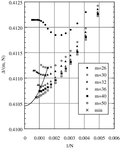
FIG. 10.: The gap $\Delta^{1}(m,N)$ in the unit of the coupling constant $J$ as a function of the number of state $m=\sum_{j}m_{j}$ kept in the IRF-DMRG calculations and the spin chain length $N$. Each cross denotes the position of minimum for a given $m$ curve.

Figure 11 shows the gap $\Delta_{2}(m,N)$, as measured by the difference between the lowest energy of $S^{T}=1$ states and that of $S^{T}=0$ states, as a function of the spin chain length $N$ and the number of states $m$ kept in the IRF-DMRG iterations. The extrapolations are performed for both $m$ and $N$ simultaneously and the upper estimated value $\Delta_{U}$ and lower one $\Delta_{L}$ are obtained by using the polynomial fits with second order and third order, respectively. The estimated Haldane gap for the $S=2$ AFH chain is $\Delta_{2}\cong 0.0878\pm 0.0016$.

IV Conclusions

The IRF-DMRG is reviewed and developed for higher integer quantum spin chain models which has a rotational symmetry. The explicit expressions of the IRF weights for the nearest neighbor spin-$S$ interaction have been derived as a function of total spin $j$. Using these IRF weights the IRF-DMRG has been applied to both $S=1$ and $S=2$ isotropic AFH quantum spin chains. With the moderate number (up to $m=90$) of states kept in the IRF-DMRG iterations, the Haldane gaps and ground state energy densities were readily calculated since the degeneracy due to the spin symmetry had been eliminated.

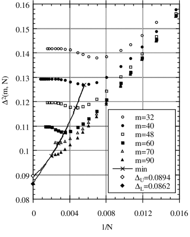
FIG. 11.: The gap $\Delta^{2}(m,N)$ in the unit of the coupling constant $J$ as a function of the number of state $m=\sum_{j}m_{j}$ kept in the IRF-DMRG calculations and the spin chain length $N$. Each cross denotes the position of minimum for a given $m$ curve. The open and solid diamonds denote upper estimated value $\Delta_{U}$ and lower one $\Delta_{L}$, respectively.

A Wigner-Eckart’s theorem

The Wigner-Eckart’s theorem is briefly reviewed to derive the IRF weights associated with general spin-$S$ interaction in the form of $\bf{S}\cdot\bf{S}^{\prime}$ in the next appendix. Most of the results presented here are already known and can be found in Ref. [4].

Let $T_{M}^{(k)}$ is an irreducible tensor operator with an angular momentum ${\bf k}$ and the third component $M(=-k,\cdots,k)$. $T_{M}^{(k)}$ commutes with the total angular momentum operator ${\bf J}$ of a system considered as

$$[J_{z},T_{M}^{(k)}] = MT_{M}^{(k)}$$ (A1)

$$[J_{x}\pm iJ_{y},T_{M}^{(k)}] = \sqrt{k(k+1)-M(M\pm 1)}T_{M\pm 1}^{(k)}.$$ (A2)

i.e., $T_{M}^{(k)}$ is transformed as a tensor under a rotational operation for the system. For example, each component of spin operator ${\bf S}$ is expressed as

$$T_{0}^{(1)} = S_{z},$$ (A3)

$$T_{\pm 1}^{(1)} = \frac{\mp 1}{\sqrt{2}}S_{\pm}.$$ (A4)

The inner product of a pair of irreducible tensors ${\bf T^{(k)}}$ and ${\bf U^{(k)}}$ is defined with

$${\bf T^{(k)}}\cdot{\bf U^{(k)}}\equiv\sum_{M=-k}^{k}(-1)^{-M}T^{(k)}_{M}U^{(k)}_{-M}.$$ (A5)

For spin operator one readily checks the following relation:

$${\bf T^{(1)}}\cdot{\bf T^{(1)}}={\bf S}\cdot{\bf S}.$$ (A6)

Wigner-Eckart’s theorem shows the matrix elements for $T_{M}^{(k)}$ are factored as a product of a configuration dependent part, which expressed as Wigner’s $3$-$j$ symbols or Clebsh-Gordan (CG) coefficients, and a configuration independent part:

$$\langle JM|T^{(k)}_{\mu}|J^{\prime}M^{\prime}\rangle\hskip 108.405pt$$ (A7)

$$=(-1)^{J-M}\left[\begin{array}[]{ccc}J&k&J^{\prime}\\ -M&\mu&M^{\prime}\end{array}\right](J||{\bf T}^{(k)}||J^{\prime}),$$ (A10)

where $(J||{\bf T}^{(k)}||J^{\prime})$ are called reduced matrix elements, which is independent of the configuration $M$ or $M^{\prime}$. Wigner’s $3$-$j$ symbol is related with CG coefficient as

$$\left[\begin{array}[]{ccc}J&k&J^{\prime}\\ -M&\mu&M\end{array}\right]=\frac{(-1)^{J-k-M^{\prime}}}{\sqrt{2J^{\prime}+1}}\langle J-\!Mk\mu|J^{\prime}-\!M^{\prime}\rangle.$$ (A11)

Once the reduced matrix elements are known, one gets the all matrix elements with only calculations for CG coefficients. For example one easily finds the reduced matrix element for spin operator ${\bf S}$ by applying the theorem Eq. (A10) to $S^{z}$, which is corresponding to $k=1$ and $\mu=0$, as the following:

$$\langle SM|T^{(1)}_{0}|SM^{\prime}\rangle=(-1)^{S-M}\left[\begin{array}[]{ccc}S&1&S\\ -M&0&M^{\prime}\end{array}\right](S||{\bf S}||S).$$ (A12)

Since the left hand side is $M\delta_{M,M^{\prime}}$, one gets

$$(S||{\bf S}||S)=\sqrt{S(S+1)(2S+1)}.$$ (A13)

The following relations [4] are used to derive the expression for the IRF-weights of general spin-$S$ chain in the next appendix:

$$\langle j_{1}j_{2}JM|{\bf T}^{(k)}_{1}\cdot{\bf T}^{(k)}_{2}|j^{\prime}_{1}j^{\prime}_{2}J^{\prime}M^{\prime}\rangle\qquad\qquad$$ (A14)

$$=\delta_{JJ^{\prime}}\delta_{MM^{\prime}}(-1)^{j_{2}+J+j^{\prime}_{1}}\left\{\begin{array}[]{ccc}j_{1}&j_{2}&J\\ j^{\prime}_{2}&j^{\prime}_{1}&k\end{array}\right\}$$ (A17)

$$\qquad\times(j_{1}||{\bf T}^{(k)}_{1}||j^{\prime}_{1})(j_{2}||{\bf T}^{(k)}_{2}||j^{\prime}_{2}),$$ (A18)

$$(j_{1}j_{2}J||{\bf T}^{(k)}_{1}||j^{\prime}_{1}j^{\prime}_{2}J^{\prime})\hskip 72.26999pt\qquad$$ (A19)

$$=\delta_{j_{2}j^{\prime}_{2}}(-1)^{j_{1}+j_{2}+J^{\prime}+k}\left\{\begin{array}[]{ccc}j_{1}&J&j_{2}\\ J^{\prime}&j^{\prime}_{1}&k\end{array}\right\}$$ (A22)

$$\qquad\times\sqrt{(2J+1)(2J^{\prime}+1)}(j_{1}||{\bf T}^{(k)}_{1}||j^{\prime}_{1}),$$ (A23)

$$(j_{1}j_{2}J||{\bf T}^{(k)}_{2}||j^{\prime}_{1}j^{\prime}_{2}J^{\prime})\hskip 72.26999pt\qquad$$ (A24)

$$=\delta_{j_{1}j^{\prime}_{1}}(-1)^{j_{1}+j^{\prime}_{2}+J+k}\left\{\begin{array}[]{ccc}j_{2}&J&j_{1}\\ J^{\prime}&j^{\prime}_{2}&k\end{array}\right\}$$ (A27)

$$\qquad\times\sqrt{(2J+1)(2J^{\prime}+1)}(j_{2}||{\bf T}^{(k)}_{2}||j^{\prime}_{2}).$$ (A28)

B IRF-weights

I here derive the IRF weights for the following Hamiltonian $H$, which is invariant under rotations.

$$H_{i,i+1}={\bf S}_{i}\cdot{\bf S}_{i+1},$$ (B1)

where ${\bf S}_{i}$ and ${\bf S}_{i+1}$ are not necessarily same. The IRF weights for the $H$ are expressed as the matrix elements

$$\langle(J_{i}S_{i+1}),J_{i+1}M_{i+1}|{\bf S}_{i}\cdot{\bf S}_{i+1}|(J^{\prime}_{i}S_{i+1}),J^{\prime}_{i+1}M^{\prime}_{i+1}\rangle,$$ (B2)

where $|(J_{i}S_{i+1}),J_{i+1}M_{i+1}\rangle$ is a state that the sum of spin angular momenta until the $(i+1)$-th spin is $J_{i+1}$ and the corresponding third component is $M_{i+1}$. The $J_{i+1}$ consists of $J_{i}$ and a spin-$S_{i+1}$ spin.

Using Eq. (A18) one finds

$$\langle(J_{i}S_{i+1}),J_{i+1}M_{i+1}|{\bf S}_{i}\cdot{\bf S}_{i+1}|(J^{\prime}_{i}S_{i+1}),J_{i+1}M_{i+1}\rangle$$ (B3)

$$=(-1)^{J_{i+1}+J_{i}+S_{i+1}}\left\{\begin{array}[]{ccc}J_{i}&S_{i+1}&J_{i+1}\\ S_{i+1}&J^{\prime}_{i}&1\end{array}\right\}$$ (B6)

$$\quad\times(S_{i+1}||{\bf S}||S_{i+1})(J_{i}||{\bf S}||J^{\prime}_{i}).$$ (B7)

Since $|J_{i})$ can be expressed as a tensor product of $J_{i-1}$ and spin-$S$, the last reduced matrix element in the above equation may be written, with the help of Eq. (A23), as

$$(J_{i}||{\bf S}||J^{\prime}_{i})=(J_{i-1}S_{i}J_{i}||{\bf S}||J^{\prime}_{i-1}S_{i}J^{\prime}_{i})\hskip 57.81621pt$$ (B8)

$$=\delta_{J_{i-1}J^{\prime}_{i-1}}(-1)^{J^{\prime}_{i}+S_{i}+J_{i-1}+1}\left\{\begin{array}[]{ccc}S_{i}&J_{i}&J_{i-1}\\ J^{\prime}_{i}&S_{i}&1\end{array}\right\}$$ (B11)

$$\quad\times\sqrt{(2J_{i}+1)(2J^{\prime}_{i}+1)}(S_{i}||{\bf S}||S_{i}).$$ (B12)

Hence the final expression is obtained as

$$R\left(\begin{array}[]{ccc}&J^{\prime}_{i}&\\ J_{i-1}&&J_{i+1}\\ &J_{i}&\end{array}\right)\hskip 144.54pt$$ (B16)

$$\equiv\langle(J_{i}S_{i+1}),J_{i+1}|{\bf S}_{i}\cdot{\bf S}_{i+1}|(J^{\prime}_{i}S_{i+1}),J_{i+1}\rangle\qquad$$ (B17)

$$=(-1)^{S_{i}+S_{i+1}+J_{i-1}+J_{i}+J^{\prime}_{i}+J_{i+1}+1}\sqrt{(2J_{i}+1)(2J^{\prime}_{i}+1)}$$ (B18)

$$\times\sqrt{S_{i}(S_{i}+1)(2S_{i}+1)}\sqrt{S_{i+1}(S_{i+1}+1)(2S_{i+1}+1)}\quad$$ (B19)

$$\times\left\{\begin{array}[]{ccc}J_{i}&S_{i+1}&J_{i+1}\\ S_{i+1}&J^{\prime}_{i}&1\end{array}\right\}\left\{\begin{array}[]{ccc}S_{i}&J_{i}&J_{i-1}\\ J^{\prime}_{i}&S_{i}&1\end{array}\right\}.$$ (B24)

1 $S=1$ nearest-neighbor interaction

There are thirteen nontrivial IRF weights R for the $S=1$ nearest neighbor spin interactions: ${\bf S}_{i}\cdot{\bf S}_{i+1}$. They can be obtained by substituting $S_{i}=S_{i+1}=1$ in Eq. (B24) and the results as a function of $j$ are summarized in Fig. 12 with diagrammatic representation. In each diagram the magnitude of spin angular momentum for the middle vertex is assumed to be $j$, and the height of each vertex represents the magnitude of the spin angular momentum that assigned to the vertex. The first diagram, for example, stands for $R\left(\begin{array}[]{ccc}&j&\\ j+1&&j+1\\ &j&\\ \end{array}\right)=\frac{-j}{j+1}$. Similar results for $S=2$ case are readily obtained with the help of a symbolic manipulation language such as mathematica.

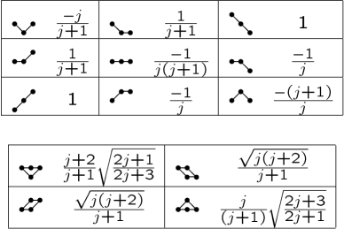
FIG. 12.: The diagrammatic representations and corresponding expressions for the IRF-weights of the $S=1$ nearest-neighbor interaction ${\bf S}_{i}\cdot{\bf S}_{i+1}$. In each diagram the hight of a vertex represents the magnitude of the spin angular momentum assigned to the vertex. The height of the (lower) middle vertex is assumed to be $j$.

REFERENCES

- [1] S. R. White, Phys. Rev. Lett. 69, 2863 (1992); Phys. Rev. B 48, 10345 (1993).
- [2] Density-Matrix Renormalization - A New Numerical Method in Physics, edited by I. Peshel, X. Wang, M. Kaulke, K. Hallberg,(Springer-Verlag, Berlin, 1999).
- [3] S. Östlund and S. Rommer, Phys. Rev. Lett. 75, 3537 (1995); S. Rommer and S. Östlund, Phys. Rev. B 55, 2164 (1997).
- [4] J. M. Roman, G. Sierra, J. Dukelsky, M. A. Martn-Delgado, J. Phys. A, Math. Gen. 31, 9729 (1998): cond-mat/9802150.
- [5] J. Dukelsky, M. A. Martn-Delgado, T. Nishino and G. Sierra, Europhys. Lett., 43 457 (1998).
- [6] G. Sierra, M. A. Martn-Delgado, cond-mat/9811170.
- [7] U. Schollwöck and T. Jolicœur, Europhys. Lett. 30, 493 (1995): cond-mat/9501115; U. Schollwöck, O. Golinelli and T. Jolicœur, Phys. Rev. B 54, 4038 (1996).
- [8] X. Wang, S. Qin and L. Yu, Phys. Rev. B 60 14529 (1999): cond-mat/9903035.
- [9] S. Qin, Y. Lin and L. Yu, Phys. Rev. B 55, 2721 (1997); S. Qin, X. Wang and L. Yu, ibid. B 56, R14251 (1997).
- [10] G. Sierra and T. Nishino, Nuclear Physics B495 505 (1997), cond-mat/9610221.
- [11] N. Flocke and J. Karwowski, Phys. Rev. B 55 8287 (1997).
- [12] R. J. Baxter, Exactly Solved Models in Statistical Mechanics (Academic Press, London, 1982).
- [13] I’ve learned this targeting method from Nishino Tomotoshi.
- [14] F. D. M. Haldane, Phys. Lett. 93A, 464 (1983); Phys. Rev. Lett. 50, 1153 (1983).
- [15] In Ref. [10] the term “super-string” is used, but I use “superblock” through out this paper.
- [16] J. B. Parkinson and J. C. Bonner, Phys. Rev. B 32, 4703 (1985); M. Takahashi, Phys. Rev. Lett. 62, 2313 (1989); S. Ma, C. Broholm, D. H. Reich, B. J. Sternlieb and R. W. Erwin, ibid. 69, 3571 (1992).
- [17] S. R. White, Phys. Rev. B 48, 3844 (1993).
- [18] I. Affleck, T. Kennedy, E. H. Lieb and H. Tasaki, Phys. Rev. Lett. 59, 799 (1987).
- [19] E. S. Sorensen and I. Affleck, Phys. Rev. Lett. 71, 1633 (1993).
- [20] The DMRG mailing lists maintained by Nishino and Hieida. Detailed information can be available from http://quattro.phys.kobe-u.ac.jp/dmrg/DMlist.html
- [21] A C++ matrix manipulation library by Robert Davies. http://nz.com/webnz/robert/nzc_nm09.html
- [22] The EGCS was the experimental GNU compiler system. It is integrated to GCC. http://egcs.cygnus.com
- [23] A stable and robust Linux-Alpha package developed by Goto Kazushige for numerical computation. It is still under development and unfortunately there is no detailed document but a brief README file in Japanese.
- [24] One of the freely available UNIX-like operating systems for Alpha CPU workstations. http://www.netbsd.org