Finite Temperature Collapse of a Bose Gas with Attractive Interactions

Abstract

We study the mechanical stability of the weakly interacting Bose gas with attractive interactions, and construct a unified picture of the collapse valid from the low temperature condensed region to the high temperature classical regime. As we show, the non-condensed particles play a crucial role in determining the region of stability. We extend our results to describe domain formation in spinor condensates.

The trapped Bose gas with attractive interactions is a novel physical system. At high densities these clouds are unstable against collapse; however at low densities they can be stabilized by quantum mechanical and entropic effects. Such stability and the subsequent collapse has been observed in clouds of degenerate ⁷Li [3]. The collapse of the Bose gas shares many features of the gravitational collapse of cold interstellar hydrogen, described by the Jeans instability [4]; related instabilities occur in supercooled vapors. Theoretical studies of the attractive Bose gas, typically numerical, have been limited to zero [5] or very low [6] temperature. Here we give a simple analytic description of the region of stability and the threshold for collapse, valid from zero temperature to well above the Bose condensation transition, and thus provide a consistent global picture of the instability. As we show, the non-condensed particles play a signficant role in the collapse at finite temperature [7]. Indeed in the normal state, collapse occurs even when no condensate exists.

Our results are summarized in the phase diagram in Fig. 1, which shows three regions: normal, Bose condensed, and collapsed. This third region is not readily accessible experimentally; the system becomes unstable at the boundary (the solid line in the figure). The attractive interactions, which drive the instability, have a characteristic energy $V=\hbar^{2}(a_{s}n)/m$ per particle, where $\hbar$ is Planck’s constant, $a_{s}$ ($=-1.45$nm for ⁷Li) is the s-wave scattering length, $n$ is the density, and $m$ is the particle mass. At low temperature the only stabilizing force is quantum pressure, arising from the zero-point motion of the particles, with a characteristic energy $E_{Q}=\hbar^{2}/mL^{2}$, where $L$ is the size of the cloud. At higher temperatures, thermal pressure, resulting from the decrease in entropy with decreasing volume of a system, also helps to stabilize the cloud. The characteristic energy scale for thermal pressure is $E_{T}=k_{B}T$, where $T$ is the temperature. Naively, the line of collapse is where $V$ becomes larger than both $E_{T}$ and $E_{Q}$. Quantum pressure rapidly decreases as the system size increases, and in the thermodynamic limit the entire condensed phase is swallowed up by the collapsed phase (cf. Fig. 2). Due to the finite system size the line separating the normal and condensed phase is not a phase transition, but rather is a rapid cross-over.

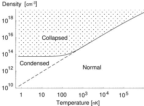
FIG. 1.: Phase diagram, density $n$ [cm^-3] versus temperature $T$ [nK], for a small cloud of attractive bosons with spatial extent $L=3.15\mu$m, scattering length $a_{s}=-1.45$nm, and atomic weight 7 (see [1]). Note the logarithmic scales. To apply these results to harmonically trapped gases, the density $n$ should be interpreted as the central density in the trap. The solid line separates the unstable (shaded) region from the stable region.

The zero temperature stability of a finite boson cloud can be understood in terms of the Bogoliubov excitation spectrum of a uniform gas [8]:

$$\omega^{2}=\left(\frac{k^{2}}{2m}\right)^{2}+gn\frac{k^{2}}{m},$$ (1)

where $g=4\pi\hbar^{2}a_{s}/m$. In the attractive case, $g<0$, all long wavelength modes with $k^{2}/2m<2|g|n$ have imaginary frequencies and are unstable. A system of finite size $L$ has modes only for $k>2\pi/L$ and will have an excitation spectrum similar to Eq. (1) for short wavelengths. Thus one expects that a zero temperature attractive Bose gas will be stable if $|g|n<\hbar^{2}\pi^{2}/mL^{2}$ [9]. We extend this analysis to finite temperature by calculating the zero frequency density-density response function $\chi(k)$. The onset of an instability in the longest wavelength mode is signaled by a divergence in $\chi(k=2\pi/L)$.

The main role of finite temperature, $T$, is to supplement quantum pressure with thermal pressure. In the limit $T\gg T_{c}$, quantum effects are negligible, and the line of collapse becomes the spinodal line of a classical liquid-gas phase transition, as characterized by Mermin [10]. To illustrate the physics of this non-degenerate regime we look for an instability in the uniform gas at zero wavevector, $k=0$, calculating the compressibility in the Hartree approximation [11], and effectively neglecting finite size effects such as quantum pressure. Within this approximation the density is given by the self-consistent solution of

$$n=\int\frac{d^{3}p}{(2\pi\hbar)^{3}}\frac{1}{e^{\beta(\varepsilon(p)-\mu)}-1},$$ (2)

with Hartree quasiparticle energies $\varepsilon(p)=p^{2}/2m+gn$. Here $\mu$ is the chemical potential, and $\beta=1/k_{B}T$. In the classical limit, this equation becomes $n=e^{\beta(\mu-gn)}/\Lambda_{T}^{3}$, where the thermal wavelength is $\Lambda_{T}=(2\pi\hbar^{2}/mk_{B}T)^{1/2}$. The compressibility is proportional to the zero wavevector density-density response function, $\chi(k=0)=-\partial n/\partial\mu$. We introduce the “bare” response, $\chi_{0}(k=0)=-\left(\partial n/\partial\mu\right)_{\varepsilon}$, where the $\varepsilon$ are held fixed; in the classical limit $\chi_{0}(0)=-\beta n$. The full response $\chi(0)$, as in the random phase approximation (RPA), is

$$\chi(k)=\frac{\chi_{0}(k)}{1-g\chi_{0}(k)};$$ (3)

in the classical limit $\chi(0)=-\beta n/(1+g\beta n)$. The collapse of the attractive system ($g<0$) is signaled by a divergence of the compressibility. In the classical limit, this divergence occurs when $|g|n=k_{B}T$ [9]. The approximations made here break down when $|\mu|\sim\hbar^{2}/mL^{2}$ and if applied outside their range of validity would erroneously predict that the instability towards collapse prevents Bose condensation from occurring.

In the experiments on ⁷Li, the atoms are held in a magnetic trap with a harmonic confining potential $V(r)=\frac{1}{2}m\omega^{2}r^{2}$, with $\omega\approx 2\pi\times 145s^{-1}$, and have a highly inhomogeneous density profile [12]. In connecting the theory of the uniform gas with the experiment, $n$ should be interpreted as the density at the center of the trap, and the system size $L$ as effectively $\sqrt{\hbar/m\omega}$ ($=3.2\mu$m). As long as $k_{B}T$ is larger than the trap energy $\hbar\omega\approx 7nK$, the geometry of the trap should play no significant role in the collapse.

We describe the system more generally using the response function $\chi(k)$ derived from the shielded potential approximation [13], as used by Szépfalusy and Kondor to study the critical behavior of collective modes [14]. This approach, a simple example of the dielectric formalism, generates an excitation spectrum which is conserving [15] and gapless [16]. At zero temperature it yields the Bogoliubov spectrum shown in Eq. (1), and above $T_{c}$ it becomes the standard RPA. Analysis in terms of Bogoliubov quasiparticles is left to a future paper.

The susceptibility has the general form, Eq. (3), with the appropriate polarization part $\chi_{0}$. Within the shielded potential approximation $\chi_{0}$ is the response of the non-interacting system. This response can be broken up into two parts, $\chi_{0}^{s}$ and $\chi_{0}^{r}$, corresponding to the condensate and non-condensate contributions [17], which at finite frequency are given by

$$\chi_{0}^{r}(k,\omega) = \int\frac{d^{3}q}{(2\pi)^{3}}\frac{f(q-k/2)-f(q+k/2)}{\omega-(\varepsilon_{q+k/2}-\varepsilon_{q-k/2})},$$ (5)

$$\chi_{0}^{s}(k,\omega) = \frac{n_{0}}{\omega-\varepsilon_{k}}-\frac{n_{0}}{\omega+\varepsilon_{k}}.$$ (6)

Here $n_{0}$ is the condensate density, $\varepsilon_{k}=k^{2}/2m$ is the free particle spectrum, and the Bose factors $f(k)$ are given by $(e^{-\beta(\varepsilon_{k}-\mu)}-1)^{-1}$.

Expanding $\chi_{0}^{r}$ in the small parameter $k\Lambda_{T}$ we derive for $T>T_{c}$,

$$g\chi_{0}^{r}(k) = -2\frac{a_{s}}{\Lambda_{T}}\left[\frac{4\pi}{k\Lambda_{T}}\arctan\left(\frac{1}{2}\left|\frac{\epsilon_{k}}{\mu}\right|^{1/2}\right)\right.$$ (9)

$$\quad\left.+g_{1/2}(e^{\beta\mu})-\left|\frac{\pi}{\beta\mu}\right|^{1/2}+{\cal O}(k\Lambda_{T})\right],$$

$$g\chi_{0}^{s}(k) = 0,$$ (10)

$$n = \frac{1}{\lambda_{T}^{3}}g_{3/2}(e^{\beta\mu}).$$ (11)

where $g_{\nu}(z)\equiv\sum_{j}z^{j}/j^{\nu}$ is the polylogarithm function. For chemical potential $\mu$ much larger in magnitude than $k_{B}T$, the system is in the classical regime, and Eq. (9) reduces to $g\chi_{0}^{r}=-\beta gn$, as was found in the Hartree approach. Below $T_{c}$ the chemical potential of the non-interacting system vanishes and the response functions are simpler:

$$g\chi_{0}^{r}(k) = -\frac{4\pi^{2}a_{s}}{k\Lambda_{T}^{2}}+{\cal O}((k\Lambda_{T})^{0}),$$ (13)

$$g\chi_{0}^{s}(k) = -16\pi\frac{a_{s}n_{0}}{k^{2}},$$ (14)

$$n = n_{0}+\frac{1}{\Lambda_{T}^{3}}\zeta(3/2),$$ (15)

with $\zeta(\nu)=g_{\nu}(1)$, the zeta function. Using these expressions we calculate the spinodal line separating the stable and unstable regions of Fig. 1 by setting $k=2\pi/L$ and solving the equation

$$\chi^{-1}\propto 1-g(\chi_{0}^{s}+\chi_{0}^{r})=0.$$ (16)

Note that the condensate response $\chi_{0}^{s}$ scales as $L^{2}$, whereas below $T_{c}$ the noncondensate response $\chi_{0}^{r}$ scales as $L$. For realistic parameters, $L$ is the largest length in the problem, so the condensate dominates the instability except when $n_{0}$ is much smaller than $n$. In Fig. 2 we plot the line of instability for various $L$.

From the above equations we calculate the maximum stable value of the condensate density $n_{0}$:

$$(n_{0})_{\rm max}=\frac{\pi}{4L^{3}}\left(\frac{L}{|a|}-\frac{L^{2}mk_{B}T}{\hbar^{2}}\right);$$ (17)

$(n_{0})_{\rm max}$ decreases linearly with temperature, eventually vanishing at $T=\hbar^{2}/mL|a|$. Conversely, the maximum total density increases rather quickly with temperature. Using parameters from the Rice experiments [3], we find

$$(N_{0})_{\rm max}=L^{3}(n_{0})_{\rm max}=1706-T/(8.8nK).$$ (18)

This result, plotted in Fig. 3, is consistent with the experiments, and agrees qualitatively with numerical mean-field calculations [6]. Quantitative agreement requires a more sophisticated treatment of the geometry. To verify the structure in Eq. (18) and to map out the phase diagram in Fig. 1, future condensate experiments will need to be performed at temperatures of several $\mu$K, an order of magnitude hotter than the current 100 to 300 nK experiments. At these temperatures the density needed for collapse is so high that inelastic two and three body processes seriously restrict the lifetime of the condensate [18]. Thus it may become necessary to work with softer traps (larger $L$), where the line of collapse lies at lower densities (see Fig. 2).

FIG. 2.: Scaling of the instability threshold with system size. Solid lines show the maximum stable density $n_{\rm max}$ for a given temperature. From the top, the system size is $L$ = 0.3, 3, 30 $\mu$m. The other parameters are the same as Fig. 1. The dashed line indicates the Bose-Einstein condensation transition. Note the three scaling regimes; at low temperature, $n_{\rm max}\sim L^{2}$, near the critical temperature $n_{\rm max}\sim L^{3/2}$, and at high temperatures $n_{\rm max}$ is independent of $L$ (see Eqs. (5) and (6)).

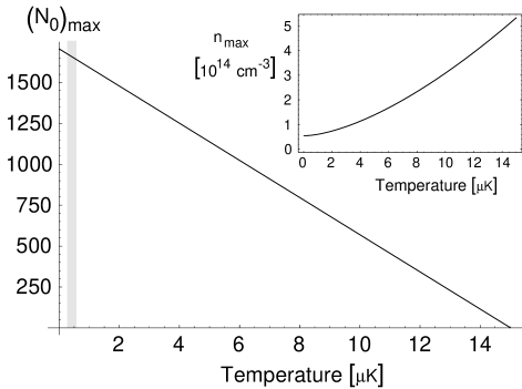
FIG. 3.: Maximum number of condensed particles as a function of temperature for the same parameters as in Fig. 1. Present experiments are performed in the shaded region. The inset shows the maximum total density for the same temperature range.

The formalism used here to discuss the collapse of a gas with attractive interactions also describes domain formation in spinor condensates, and gives a nice qualitative understanding of experiments at MIT [20] in which optically trapped ²³Na is placed in a superposition of two spin states. Although all interactions in this system are repulsive, the two different spin states repel each other more strongly than they repel themselves, resulting in an effective attractive interaction. The collapse discussed earlier becomes, in this case, an instability towards phase separation and domain formation. The equilibrium domain structure is described in [21]. Here we focus on the formation of metastable domains.

The ground state of sodium has hyperfine spin $F=1$. In the experiments the system is prepared so that only the states $|1\rangle=|F=1,m_{F}=1\rangle$ and $|0\rangle=|F=1,m_{F}=0\rangle$ are involved in the dynamics. The effective Hamiltonian is then

$$H=\int\!\!d^{3}r\,\frac{\nabla\psi_{i}^{\dagger}\cdot\nabla\psi_{i}}{2m}+V(r)\psi_{i}^{\dagger}\psi_{i}+\frac{g_{ij}}{2}\psi^{\dagger}_{i}\psi^{\dagger}_{j}\psi_{j}\psi_{i}.$$ (19)

where $\psi_{i}$ ($i=0,1$) is the particle destruction operator for the state $|i\rangle$; summation over repeated indices is assumed. The effective interactions, $g_{ij}=4\pi\hbar^{2}a_{ij}/m$, are related to scattering amplitudes $a_{F=0}$ and $a_{F=2}$, corresponding to scattering in the singlet ($F_{1}+F_{2}=0$) and quintuplet ($F_{1}+F_{2}=2$) channel by [20, 21, 22]:

$$\tilde{a}\equiv a_{11}=a_{01}=a_{10}=a_{F=2},$$ (21)

$$\delta a\equiv a_{11}-a_{00}=(a_{F=2}-a_{F=0})/3.$$ (22)

Numerically, $\tilde{a}=2.75$nm and $\delta a=0.19$nm. We introduce $\tilde{g}=4\pi\hbar^{2}\tilde{a}/m$ and $\delta g=4\pi\hbar^{2}\delta a/m$. In the mean field approximation, the interaction in Eq. (19) becomes a function of $n_{m=0}$ and n, the density of particles in the state $|0\rangle$ and the total density, respectively:

$$\langle H_{int}\rangle=\int\!\!d^{3}r\,\left(\frac{\tilde{g}}{2}n^{2}-\frac{\delta g}{2}n_{m=0}^{2}\right),$$ (23)

which shows explicitly the effective attractive interaction. Initially the condensate is static withdensity $n=10^{14}{\rm cm}^{-3}$, and all particles in state $|1\rangle$. A radio frequency pulse places half of the atoms in the $|2\rangle$ state without changing the density profile. Subsequently the two states phase separate and form domains from 10 to 50 $\mu$m thick. The trap plays no role here, so we can neglect $V(r)$ in Eq. (19) and consider a uniform cloud.

Linearizing the equations of motion with an equal density of particles in each state, we find two branches of excitations corresponding to density and spin waves [23],

$$\omega_{ph}^{2} = \left(\frac{k^{2}}{2m}\right)^{2}+\tilde{g}n\frac{k^{2}}{m}+{\cal O}(\delta g),$$ (25)

$$\omega_{sp}^{2} = \left(\frac{k^{2}}{2m}\right)^{2}-\delta g\,n\frac{k^{2}}{4m}+{\cal O}((\delta g)^{2}).$$ (26)

Since $\delta g>0$ we see the appearance of spin excitations with imaginary frequency. The mode with the largest imaginary frequency grows most rapidly, and the width of the domains formed should be comparable to the wavelength $\lambda$ of this mode. By minimizing Eq. (26) one finds $\lambda=\sqrt{2\pi/n\,\delta a}=10\mu$m, in rough agreement with the observed domain size.

The authors are grateful to the Ecole Normale Supérieure in Paris, and the Aspen Center for Physics, where this work was carried out. We owe special thanks to Eugene Zaremba and Dan Sheehy for critical comments. The research was supported in part by the Canadian Natural Sciences and Engineering Research Council, and National Science Foundation Grant No. PHY98-00978. This work was facilitated by the Cooperative Agreement between the University of Illinois at Urbana-Champaign and the Centre National de la Recherche Scientifique.

REFERENCES

- [1] Electronic address: emueller@physics.uiuc.edu
- [2] Electronic address: gbaym@uiuc.edu
- [3] C.A. Sackett, H.T.C. Stoof, and R.G. Hulet, Phys. Rev. Lett. 80 2031, (1998); C.A. Sackett, C.C. Bradley, M. Welling, and R.G. Hulet, Appl. Phys. B 65 433, (1997); C.C. Bradley, C.A. Sackett, and R.G. Hulet, Phys. Rev. Lett. 78 985, (1997); C.C. Bradley, C.A. Sackett, and R.G. Hulet, Phys. Rev. A 55 3951, (1997).
- [4] For elementary discussions of the Jeans instability see, e.g., R. Bowers, and T. Deeming Astrophysics II; Interstellar Matter and Galaxies (Jones and Bartlett, Sudbury, MA, 1984).
- [5] P.A. Ruprecht, M.J. Holland, K. Burnett, and M. Edwards, Phys.Rev. A 51, 4704 (1995); G. Baym and C. J. Pethick, Phys. Rev. Lett. 76 6 (1996).
- [6] M.J. Davis, D.A.W. Hutchinson, and E. Zaremba, J. Phys. B 32, 3993 (1999); T. Bergeman, Phys. Rev. A 55, 3658 (1997); M. Houbiers and H.T.C. Stoof, Phys. Rev. A 54, 5055 (1996); P.A. Ruprecht, M.J. Holland, K. Burnett, and M. Edwards, Phys. Rev. A 51, 4704 (1995).
- [7] Previous theoretical studies [6] focused on the stability of the condensate at very low temperatures and in a regime where the density of non-condensed particles is much smaller than the condensate density. These studies found that the non-condensed particles play a very small role in the collapse. For example, Stoof et al. concluded that the non-condensed particles are involved in the collapse only in so far as they change the geometry of the effective potential felt by the condensate. In this low temperature regime our results are consistent with these previous works.
- [8] N.N. Bogoliubov, J. Phys. USSR, 11, 23 (1947)
- [9] Up to a factor of order unity, this result can be derived through dimensional analysis.
- [10] N.D. Mermin, Ann. Phys. 18, 421, 454 (1962); 21, 99 (1963).
- [11] We neglect exchange here to aid comparison with the RPA, which extends Hartree theory to finite wavevector and frequency. It is straightforward to add exchange to the formalism, but such details needlessly obscure the discussion here.
- [12] The trap used is slightly asymmetric, and the frequency quoted here is the geometric mean of the three frequencies; see [3].
- [13] L.P. Kadanoff and G. Baym, Quantum Statistical Mechanics (W.A. Benjamin, New York, 1962).
- [14] P. Szépfalusy and I. Kondor, Ann. Phys. 82, 1 (1974).
- [15] G. Baym, Phys. Rev. 127, l39l (1962).
- [16] A. Griffin, Excitations in a Bose-Condensed Liquid (Cambridge University Press, NY, 1993).
- [17] As used by Szépfalusy and Kondor [14], and denote singular and regular.
- [18] At a temperature of , a m cloud of 7Li collapses at a density of . At such a high density the dominant decay mechanism is 3-body collisions, giving a lifetime . Using the theoretical estimate [19], , we find that . At the lifetime is only .
- [19] A. J. Moerdijk, H. M. J. M. Boesten, and B. J. Verhaar, Phys. Rev. A 53, 916 (1996); C. A. Sackett, J. M. Gerton, M. Welling, and R. G. Hulet, Phys. Rev. Lett. 82, 876 (1999).
- [20] H.-J. Miesner, D. M. Stamper-Kurn, J. Stenger, S. Inouye, A. P. Chikkatur, and W. Ketterle, Phys. Rev. Lett. 82, 2228 (1999).
- [21] T. Isoshima, K. Machida, and T. Ohmi, preprint,cond-mat/9905182.
- [22] T.-L. Ho, Phys. Rev. Lett. 81, 742 (1998).
- [23] Similar excitation spectra are found in E.V. Goldstein and P. Meystre, Phys. Rev. A 55, 2935 (1997).