$B(H)$ Constitutive Relations Near $H_{c1}$ in Disordered Superconductors

Abstract

We provide a self-contained account of the $B$ vs. $H$ constitutive relation near $H_{c1}$ in Type II superconductors with various types of quenched random disorder. The traditional Abrikosov result $B\sim[\ln(H-H_{c1})]^{-2}$, valid in the absence of disorder and thermal fluctuations, changes significantly in the presence of disorder. Moreover, the constitutive relations will depend strongly on the type of disorder. In the presence of point disorder, $B\sim(H-H_{c1})^{3/2}$ in three-dimensional (thick) superconductors, as shown by Nattermann and Lipowsky. In two-dimensional (thin film) superconductors with point disorder, $B\sim(H-H_{c1})$. In the presence of parallel columnar disorder, we find that $B\sim\exp[-C_{3}/(H-H_{c1})]$ in three dimensions, while $B\sim\exp[-C_{2}/(H-H_{c1})^{1/2}]$ in two dimensions. In the presence of nearly isotropically splayed disorder, we find that $B\sim(H-H_{c1})^{3/2}$ in both two and three dimensions.

I Introduction

The physics of vortex lines in high-temperature superconductors has attracted much experimental and theoretical interest [1]. The competition between interactions, pinning, and thermal fluctuations gives rise to a wide range of novel phenomena that are both interesting in their own right and technologically important. Here, we focus primarily on the effects of disorder on vortex behavior, phenomena which are also important for low-temperature Type II superconductors. In a disorder-free sample, vortex lines always flow in response to a current, leading to a resistance even at arbitrarily small currents. By contrast, defects in superconductors attract vortex lines. Just as a few nails can hold a carpet in place, an entire vortex line system can be held in place by a few defects, leading to a large critical current—provided the vortices are in a solid phase, where they are held in place relative to each other by their mutual repulsion, which gives rise to a shear modulus. If the temperature is raised so that the vortices are in a liquid state, then vortices held in place by the disorder are pinned, but the other vortices can flow around them, leading again to zero critical current.

In the case of the high-temperature superconductors, disorder is naturally present in the form of oxygen vacancies. The quantity of such vacancies can be altered by changing the doping of the crystal, i.e., by introducing more or less oxygen during the growth process. Such changes can have a strong impact on the pinning of the vortices, and hence on the critical current. Substitutional defects can play a similar role in low-temperature superconductors.

Artificial defects added to superconductors are particularly effective in increasing the critical current. Of special note are columnar defects, which are generated by bombarding the sample with heavy ions that produce damage tracks in their wake [2, 3, 4, 5, 6]. These tracks pin vortices strongly because their width ($\sim 60\AA$) is comparable to the vortex core size ($\sim 20\AA$). When the columnar pins are aligned with the direction of the magnetic field (and hence with the vortex lines) a large increase in the critical current is observed.

However, an even greater increase in the critical current is observed when the columns are splayed, i.e., they are not all oriented in the same direction [7, 8, 9]. The superior pinning properties of columnar defects with controlled splay was predicted theoretically based on expected reduction in a variable-range hopping vortex transport mechanism and enhanced vortex entanglement due to splay [10, 11]. Despite the technological importance, much remains to be done in order to understand the behavior of vortex lines in the presence of splayed columnar disorder.

Even at high temperatures, when the analysis is expected to be most tractable, standard approaches seem to break down and give nonsensical results. For example, the boson mapping [12, 13, 14] works quite well in describing many of the properties of vortex lines in the presence of point or unsplayed columnar disorder. This approach utilizes a formal correspondence between vortex trajectories and the world lines of fictitious quantum-mechanical bosons in two dimensions. In this analogy, the temperature $T$ plays the role of Planck’s constant $\hbar$, the bending energy (or line tension) $g$ plays the role of the boson mass $m$, and the length of the sample $L$ corresponds to $\beta\hbar$ for the bosons. The analogy works best in the $L\rightarrow\infty$ limit, which corresponds to the $T\rightarrow 0$ limit for the bosons. In this limit, in the absence of disorder and interactions, the bosons should form a condensate. In the presence of disorder or interactions, some “bosons” are kicked out of the condensate, resulting in a condensate density $n_{0}$ which is less than the total density $n$. For vortex lines, the “condensate density” is a measure of the degree of entanglement [12, 13, 15]. This condensate density can be calculated for the various types of disorder discussed above. It is well-behaved for point and unsplayed columnar disorder, but in the presence of even weak splayed columnar disorder, $n_{0}$ diverges [15], suggesting that the boson mapping is flawed in the presence of splayed columnar disorder. Indeed, Täuber and Nelson [15] conclude that the super-diffusive wandering of the flux lines causes the mapping onto non-relativistic bosons to break down. Unfortunately, this mapping—which has provided many insights for the cases of no disorder, point disorder, and unsplayed columnar defects—seems to be less suitable for understanding the behavior of vortex lines in the presence of splayed columnar disorder.

Here, we focus on the behavior of vortex lines near $H_{c1}$, where the lines are dilute. In particular, we predict the $B(H)$ constitutive relation for vortex lines in the presence of the various types of disorder discussed above. We begin by reviewing the traditional Abrikosov result, expected to hold in the absence of disorder and thermal fluctuations. Each vortex that enters the sample will gain a free energy proportional to $(H-H_{c1})$ per unit length. However, there is an energy cost due to repulsive interactions between any two vortices proportional to $\frac{1}{\sqrt{r}}\exp(-r/{\lambda})$ for $r\gg\lambda$, where $r$ is the distance between the vortices and $\lambda$ is the London penetration depth. In the dilute limit, the interactions with nearest neighbors will dominate over interactions with more distant neighbors, and the free energy density is given by

$$f=-c_{1}(H-H_{c1})n+c_{2}n^{5/4}e^{-c_{3}/\sqrt{n}},$$ (1.1)

where $n$ is the density of vortices, and $c_{1}$, $c_{2}$, and $c_{3}$ are constants that can be determined in terms of the vortex parameters [16]. (We leave them general here to better elucidate the structure of the argument.) Upon minimizing $f$ with respect to $n$, we obtain

$$n=\left\{\frac{c_{3}}{\ln\left[\frac{c_{2}c_{3}}{2c_{1}n^{1/4}}\frac{1}{(H-H_{c1})}\right]}\right\}^{2}.$$ (1.2)

The dominant behavior may be obtained by substituting $n\propto c_{3}^{2}$ on the right hand side, so that the magnetic field (given by $B=n\phi_{0}$, where $\phi_{0}$ is the flux quantum) varies inversely as the square of the logarithm of $H-H_{c1}$. Plugging in the relevant parameters $c_{1}$, $c_{2}$, and $c_{3}$ for a triangular lattice, one finds [17, 16]

$$n=\frac{2\phi_{0}}{\sqrt{3}\lambda^{2}}\left\{\frac{1}{\ln\left[\frac{3\phi_{0}}{4\pi\lambda^{2}}\frac{1}{(H-H_{c1})}\right]}\right\}^{2}.$$ (1.3)

In the presence of disorder, Eq. (1.3) will be modified. With point disorder, we obtain $B\sim(H-H_{c1})$ (as calculated [18, 19] and measured by Bolle et al. [18]) in 1+1 dimensional samples, where the vortices only have one direction transverse to the magnetic field in which they can wander (see Fig. 1). In 2+1 dimensional samples (Fig. 2), we obtain $B\sim(H-H_{c1})^{3/2}$, in agreement with calculations done by Nattermann and Lipowsky [20]. In the presence of splayed columnar defects, we find that $B\sim(H-H_{c1})^{3/2}$ both for 1+1 dimensional (Fig. 3) and 2+1 dimensional (Fig. 4) samples. For columnar disorder with unbound disorder strength, Larkin and Vinokur [21] argue that $B\sim e^{C(H-H_{c1})}$ in 2+1 dimensions. However, we show that for the more physical case of bounded disorder, $B\sim\exp[-C_{3}/(H-H_{c1})]$ in 2+1 dimensions (Fig. 5), while $B\sim\exp[-C_{2}/(H-H_{c1})^{1/2}]$ in 1+1 dimensions (Fig. 6). In addition to these relations, we also estimate the prefactors (up to factors of order unity) in terms of physical constants such as the temperature, the disorder strength, and the superconducting coherence length. These prefactors are important for comparisons with experiment.

FIG. 1.: A vortex line in a 1+1 dimensional sample of width $W$ in the presence of point disorder.

FIG. 2.: A vortex line in a 2+1 dimensional sample in the presence of point disorder.

FIG. 3.: A vortex line in a 1+1 dimensional sample of width $W$ in the presence of splayed columnar disorder.

FIG. 4.: A vortex line in a 2+1 dimensional sample in the presence of splayed columnar disorder.

FIG. 5.: A vortex line in a 1+1 dimensional sample of width $W$ in the presence of parallel columnar disorder.

FIG. 6.: A vortex line in a 2+1 dimensional sample in the presence of parallel columnar disorder.

A recent torsional oscillator experiment carried out by Bolle et al. [18] confirms that $B\sim(H-H_{c1})$ for vortex lines in two dimensions in the presence of point disorder. The experiment was done by attaching a thin sheet of superconducting 2H-NbSe₂ to a high-$Q$ micro-electromechanical device, and measuring the resonance frequency of torsional oscillations of the sample. Because a sample with a magnetic moment ${\bf M}$ in a field ${\bf H}$ exerts an additional torque ${\bf\tau}={\bf M}\times{\bf H}$ on the oscillator, the magnetic field which penetrates and becomes trapped in the sample can be probed by finding shifts in the resonance frequency as a function of applied field $H$. Small jumps in the frequency as a function of applied field were observed [18], which were attributed to individual vortices entering the sample. By counting the number of jumps as a function of $H$, these authors obtained $B\sim(H-H_{c1})$. In the presence of parallel or splayed columnar disorder, the $B$ vs. $H$ curve could be measured by a very similar experiment, where the sample was first irradiated isotropically by heavy ions to produce the required disorder. In three dimensions, a similar experiment could be done using a long thin needle-shaped sample to avoid demagnetizing effects. For point disorder, this experiment was done in the 1960’s with ambiguous results [22]. In particular, work by Finnemore et al. [23] on Niobium samples seems to indicate $B\sim(H-H_{c1})^{x}$, with $x>1$. However, the decades-old data is too rough to allow quantitative comparison with the prediction for point disorder $B\sim(H-H_{c1})^{3/2}$.

We approach these problems differently for the different types of disorder. Parallel columnar disorder localizes vortices into finite transverse regions of the sample in both 1+1 and 2+1 dimensions. Therefore, at low densities, the vortices can easily avoid paying a large cost associated with their mutual repulsion if they are located in different areas of the sample. In the language of the boson mapping described above, we can approximate the intervortex interactions as merely restricting the occupancy of any given localized state to precisely one boson [13, 24]. The form of the $B(H)$ constitutive relation is then determined by the low energy tails of the density of states. This idea is explored further in Sec. III D.

By contrast, as discussed in Sec. II, in the presence of point disorder or splayed columnar disorder, noninteracting vortices will be in extended states. As such, repeated collisions between vortices play a crucial role in determining the $B(H)$ constitutive relation, as the intervortex interactions attempt to localize each vortex into a cage surrounded by their neighbors. The energy lost due to restricted vortex wandering will determine $B(H)$. We investigate this case more fully beginning in Sec. II with the problem of a single flux line superimposed on a background of disorder. The partition function describing a flux line can be mapped onto the noisy Burger’s, or KPZ, equation describing the fluctuations of an elastic interface in the presence of a random space and time dependent potential influencing the interface’s progress [25]. This problem has been studied extensively for random potentials uncorrelated in space and time (appropriate to point disorder for the vortex lines) [26, 27, 25], but more recently has also been investigated for correlated potentials [28, 29, 30]. Provided we restrict ourselves to the case where the splayed columnar defects are nearly isotropically oriented, we can use previous results for the wandering exponent $\zeta$, which describes how far the vortex line wanders transverse to the magnetic field in a distance $l$ in the field direction by the formula $\left\{\overline{[{\bf r}(l)-{\bf r}(0)]^{2}}\right\}^{1/2}\sim l^{\zeta}$, where ${\bf r}(z)$ labels the transverse coordinates of the flux line. Columnar defects with an approximately isotropic distribution of splay can be created by using neutrons or protons to trigger fission of, e.g., bismuth nuclei in BSCCO [31].

In Sec. III, we develop an approximate theory for a dilute set of vortex lines in the presence of point and splayed columnar disorder. We first derive the scaling of $B$ vs. $H$, and then focus on the prefactor of this relation. In some experiments [7, 8, 9], the columns do not traverse the entire sample, so we also consider the effect that finite column size will have on our predictions. Specifically, we expect a crossover from the point disorder behavior at extremely weak $H-H_{c1}$ to the splayed columnar behavior at somewhat larger $H-H_{c1}$.

II Single vortex line

A Model

We begin with a model free energy for a single vortex line in a $d$ dimensional sample of thickness $L$. We label the direction of the magnetic field by $\tau$, and the transverse position of the line at $\tau$ by a $d-1$ dimensional vector ${\bf r}(\tau)$. The free energy then reads [1, 13]:

$$F[{\bf r}(\tau)]=\frac{1}{2}g\int_{0}^{L}\left(\frac{d{\bf r}}{d\tau}\right)^{2}d\tau+\int_{0}^{L}V[{\bf r}(\tau),\tau]d\tau,$$ (2.1)

where $g$ is the line tension. The pinning potential $V[{\bf r},\tau]$ arises due to the interaction with, say, point disorder or splayed columnar defects. Its mean value merely affects the average field $H_{c1}$ at which vortex lines will penetrate the sample, so we subtract it out, and assume that $\overline{V[{\bf r},\tau]}=0$. We further assume that the noise is Gaussian with a correlator

$$\Delta({\bf r}-{\bf r^{\prime}},\tau-\tau^{\prime})=\overline{V[{\bf r},\tau]V[{\bf r^{\prime}},\tau^{\prime}]}.$$ (2.2)

We focus on the case of “nearly isotropic” splay. This is the defect correlator for a set of randomly tilted columnar pins, each described by a trajectory ${\bf r}(\tau)={\bf R}+{\bf v}\tau$ with a Gaussian distribution of the tilts ${\bf v}$, $P[{\bf v}]\propto e^{-v^{2}/2v_{D}^{2}}$ in the limit $v_{D}\rightarrow\infty$ [10]. For nearly isotropic splay, the Fourier transform of the correlator, defined by

$$\Delta({\bf k},\omega)=\int d^{d-1}{\bf r}\int_{0}^{L}d\tau\Delta({\bf r},\tau)e^{-i({\bf k}\cdot{\bf r}-\omega\tau)},$$ (2.3)

is given by $\Delta/k$ [10, 15], which differs from the truly isotropic limit $\Delta/(k^{2}+\omega^{2})^{1/2}$. However, using the correlator for nearly isotropic splay simplifies the calculations significantly. In the language of the noisy Burger’s (or KPZ) equation, truly isotropic splay has both spatial and temporal correlations, while nearly isotropic splay has only spatial correlations. By focusing on the nearly isotropic splay, we can therefore rely on work done on the KPZ equation with spatially correlated disorder and avoid the more complicated case of temporal disorder. Moreover, we believe that this difference should not affect the physical implications at large length scales significantly [32].

The partition function associated with the free energy of Eq. (2.1),

$$\mathcal{Z}({\bf r},\tau)=\int\mathcal{D}{\bf r}^{\prime}(\tau^{\prime})\mathit{e}^{-F[{\bf r}^{\prime}(\tau^{\prime})]/T},$$ (2.4)

i.e., the path integral of the Boltzmann factor $e^{-F[{\bf r}^{\prime}(\tau^{\prime})]/T}$ over all vortex trajectories ${\bf r}^{\prime}(\tau^{\prime})$ running from $\tau^{\prime}=0$ to position ${\bf r}(\tau)$ at $\tau^{\prime}=\tau$, obeys the differential equation

$$T\frac{\partial\mathcal{Z}({\bf r},\tau)}{\partial\tau}=\left[\frac{T^{2}}{2g}\nabla^{2}+V({\bf r},\tau)\right]\mathcal{Z}({\bf r},\tau).$$ (2.5)

Eq. (2.5) can be further transformed by means of the Cole-Hopf transformation (similar to the WKB transformation in quantum mechanics)

$$\mathcal{Z}({\bf r},\tau)=\exp\left[\mathrm{\Phi}({\bf r},\tau)\right]$$ (2.6)

into

$$T\frac{\partial\Phi}{\partial\tau}=\frac{T^{2}}{2g}\nabla^{2}\Phi+\frac{T^{2}}{2g}(\nabla\Phi)^{2}+V({\bf r},\tau).$$ (2.7)

This equation, known as the KPZ [27], or noisy Burger’s equation [26], has been studied in the case of uncorrelated (point-like) disorder in a great variety of contexts. It was studied by Forster, Nelson, and Stephen [26] as a model for the velocity fluctuations in a randomly stirred, $(d-1)$-dimensional turbulent fluid. Later, it reappeared as a model for surface roughening proposed by Kardar, Parisi, and Zhang [27]. In this context, it has inspired a great deal of work, summarized in a review article by Halpin-Healy and Zhang [25].

There have also been investigations of the properties of this equation with correlated disorder $\Delta({\bf k})=\Delta/k^{2\rho}$ in the context of surface roughening. However, to date, there has not been any reliable characterization of the exponents for the entire $d$ vs. $\rho$ space. Medina, et al. [28] have found results that seem to be accurate in two dimensions [33]. Halpin-Healy [29] has obtained results that are accurate in two dimensions, and may describe the behavior for sufficiently small $\rho$ in higher dimensions as well. Recently, Frey, et al. [30] have found exact exponent solutions not only in two dimensions but also for sufficiently large powers of $\rho$ in higher dimensions. (It is by reference to these exact results that we judge the accuracy of Medina, et al. and Halpin-Healy’s results.) Although they are not able to obtain exact results for all $d$ and $\rho$, Frey, et al. make a plausible conjecture for the behavior at smaller values of $\rho$ that is in agreement with Halpin-Healy’s short range results and with numerical simulations [34].

Our purpose here is to adapt this work to vortex lines in the presence of splayed columnar disorder, and explain some of the consequences for experiments. The application of the results for point disorder to experiments [18] is also reviewed. In Sec. II B, we set the stage for a more detailed discussion with a simple, self-contained renormalization group treatment that gives results in agreement with Frey, et al.’s exact results in its range of applicability. In Sec. II C, we discuss the limitations of this approach.

B Renormalization group

1 Scaling

To understand the vortex wandering at long length scales, we use the renormalization group method of Ref. [26] to integrate out the short-distance behavior. Since, under renormalization, the coefficients of the $\nabla^{2}\Phi$ term and the $(\nabla\Phi)^{2}$ will no longer remain identical, we replace Eq. (2.7) by the more conventional notation

$$\frac{\partial\Phi}{\partial\tau}=\nu\nabla^{2}\Phi+\frac{\lambda}{2}(\nabla\Phi)^{2}+V({\bf r},\tau),$$ (2.8)

where initially $\nu=2\lambda=T/2g$, and we have absorbed a factor of $T$ into $V$ so that $\Delta({\bf k})=\Delta/(T^{2}k)$. We generalize to correlated disorder $\Delta({\bf k})=\Delta/(T^{2}k^{2\rho})$. It is instructive to generalize the correlator this way, because then not only does $\rho=1/2$ describe nearly isotropic splayed columnar disorder, but $\rho=0$ generates the results for point disorder as well. This renormalization group will be based around a perturbation series in powers of $\lambda$.

We first rescale Eq. (2.8) by a scale factor $b$, with

$${\bf r} \rightarrow b{\bf r},$$ (2.9)

$$\tau \rightarrow b^{z}\tau,$$ (2.10)

$$\Phi \rightarrow b^{\chi}\Phi,$$ (2.11)

where $z$ and $\chi$ will eventually be chosen to keep various coupling constants fixed under the renormalization procedure. Since $z$ describes the ratio of the scaling in the timelike direction with that in the spacelike direction, $\zeta=1/z$ is exactly the wandering exponent that we are looking for. Upon inserting these transformations into Eq. (2.8), we see that the equation remains invariant under these changes provided we rescale $\nu$, $\lambda$, and $\Delta$ via

$$\nu \rightarrow b^{z-2}\nu,$$ (2.12)

$$\lambda \rightarrow b^{\chi+z-2}\lambda,$$ (2.13)

$$\Delta \rightarrow b^{2\rho+1-d+z-2\chi}\Delta.$$ (2.14)

In the absence of the nonlinearity (i.e., $\lambda=0$), the equation becomes completely scale invariant if we choose $z=2$ and $\chi=(2\rho+3-d)/2$. However, any small $\lambda$ then rescales according to

$$\lambda\rightarrow b^{(2\rho+3-d)/2}\lambda,$$ (2.15)

and thus the nonlinear term will be relevant for $d<2\rho+3$ (i.e., $d<4$ for splayed columnar disorder and $d<3$ for point disorder). For $d>2\rho+3$, we expect the mean field exponents displayed in Eq. (2.12–2.14) to be accurate, and $\zeta=1/2$. However, in the physical situation of interest, $d\leq 2\rho+3$ and we expect the scaling exponents to change due to the nonlinearity.

2 Perturbation theory

To understand the case $d\leq 2\rho+3$, we rewrite Eq. (2.8) in Fourier space via the definition

$$\Phi({\bf k},\omega)=\int d^{d-1}{\bf r}\int_{0}^{L}d\tau\Phi({\bf r},\tau)e^{-i({\bf k}\cdot{\bf r}-\omega\tau)},$$ (2.16)

obtaining

$$\Phi({\bf k},\omega)=G_{0}({\bf k},\omega)V({\bf k},\omega)-\frac{\lambda}{2}G_{0}({\bf k},\omega)\int d^{d-1}{\bf k^{\prime}}\int_{0}^{L}d\omega^{\prime}{\bf k^{\prime}}\cdot({\bf k}-{\bf k^{\prime}})\Phi({\bf k^{\prime}},\omega^{\prime})\Phi({\bf k}-{\bf k^{\prime}},\omega-\omega^{\prime}),$$ (2.17)

where

$$G_{0}({\bf k},\omega)=\frac{1}{-i\omega+\nu k^{2}}.$$ (2.18)

We define a renormalized Green’s function $G({\bf k},\omega)$ via

$$\Phi({\bf k},\omega)\equiv G({\bf k},\omega)V({\bf k},\omega)$$ (2.19)

and calculate $G({\bf k},\omega)$ perturbatively in $\lambda$. The perturbation series can be summarized diagrammatically by giving graphical representations to the renormalized and bare propagators $G({\bf k},\omega)$ and $G_{0}({\bf k},\omega)$, the disorder $V({\bf k},\omega)$, the interaction, and the disorder correlator $\Delta({\bf k})$ as shown in Fig. 7. As expressed in Eq. (2.19), $\Phi({\bf k},\omega)$ is represented by a double arrow followed by a cross to represent the disorder. Eq. (2.17) can then be represented diagrammatically as in Fig. 8. We obtain an iterative solution by substituting Eq. (2.17) for each of the $\Phi({\bf k},\omega)$ terms appearing on the right hand side of Eq. (2.17), thereby obtaining an iterative series in powers of $\lambda$. The result for the renormalized propagator is presented diagrammatically (to second order in $\lambda$) in Fig. 9.

FIG. 7.: The definitions of the graphical elements of our perturbation series. (a) represents the renormalized propagator $G({\bf k},\omega)$, (b) represents the bare propagator $G_{0}({\bf k},\omega)$, (c) represents the noise $V({\bf k},\omega)$, (d) represents the interaction $-\frac{\lambda}{2}\int{\bf q}\cdot({\bf k}-{\bf q})$, and (e) represents the disorder correlator $2\Delta({\bf k})$.

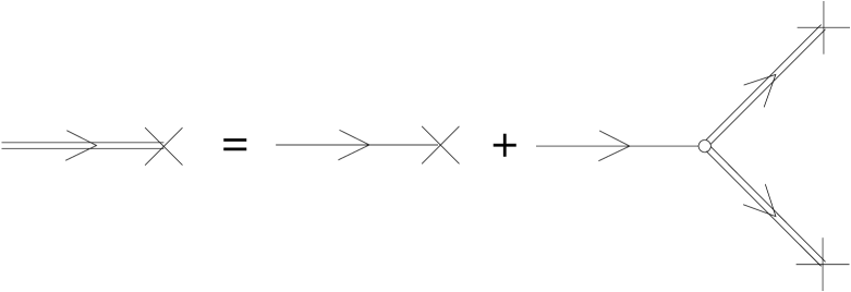
FIG. 8.: Diagrammatic representation of Eq. (2.17).

FIG. 9.: Iterated version of Eq. (2.17) to second order in $\lambda$.

We wish to use this perturbation theory to calculate renormalized versions of the parameters $\nu$, $\lambda$, and $\Delta$ (which we will denote by $\tilde{\nu}$, $\tilde{\lambda}$, and $\tilde{\Delta}$ respectively). We define $\tilde{\nu}$ by

$$\lim_{{\bf k}\rightarrow{\bf 0}}G({\bf k},0)=\frac{1}{\tilde{\nu}k^{2}}$$ (2.20)

Upon multiplying Eq. (2.17) (or its diagrammatic equivalent, Fig. 8) by $V(-{\bf k},-\omega)$ and averaging over the noise [35], we obtain the equation for the renormalized propagator represented diagrammatically to one loop order in Fig. 10.

FIG. 10.: Diagrammatic expansion of the renormalized propagator, to the one-loop order.

We define $\tilde{\lambda}$ via a renormalized vertex that contains the effects of the interactions, shown on the left hand side of Fig. 11. The vertex amplitude, in the limit of small ${\bf k}$, ${\bf q}$, $\omega$, and $\Omega$, is given by

$$-\frac{\tilde{\lambda}}{2}{\bf q}\cdot({\bf k}-{\bf q})G_{0}({\bf k},\omega)G_{0}({\bf q},\Omega)G_{0}({\bf k}-{\bf q},\omega-\Omega),$$ (2.21)

and serves as the definition of $\tilde{\lambda}$. Expanding in terms of the bare quantities, we obtain the equation determining $\tilde{\lambda}$ to one loop, shown in Fig. 11.

FIG. 11.: Diagrammatic expansion of the renormalized vertex, to the one-loop order.

We define the renormalized noise correlator $\tilde{\Delta}$ by

$$\overline{\Phi^{*}({\bf k},\omega)\Phi({\bf k},\omega)}\equiv 2\tilde{\Delta}({\bf k})G({\bf k},\omega)G({-\bf k},-\omega)$$ (2.22)

in the limit of ${\bf k}\rightarrow{\bf 0}$ and $\omega\rightarrow 0$, where

$$\tilde{\Delta}({\bf k})=\frac{\tilde{\Delta}}{T^{2}k^{2\rho}}.$$ (2.23)

Expanding in terms of the bare quantities gives rise to Fig. 12.

FIG. 12.: Diagrammatic expansion of the renormalized noise correlator, to the one-loop order.

For the case $\rho=0$, diagrams like these are expressed in integral form and evaluated in detail in Ref. [26] and, e.g., by Barabási and Stanley [36]. The case $\rho\neq 0$ does not produce any new complications, so we simply report the results:

$$\tilde{\nu} = \nu\left[1-\frac{\lambda^{2}\Delta}{T^{2}\nu^{3}}\frac{d-2\rho-3}{4(d-1)}K_{d-1}\int_{0}^{\Lambda}dqq^{d-2\rho-4}\right]$$ (2.24)

$$\tilde{\lambda} = \lambda$$ (2.25)

$$\tilde{\Delta} = \Delta\left[1+\delta_{\rho,0}\frac{\lambda^{2}\Delta}{T^{2}\nu^{3}}\frac{K_{d-1}}{4}\int_{0}^{\Lambda}dqq^{d-4}\right],$$ (2.26)

where $\Lambda$ is a cutoff in momentum space and $K_{d}$ is the surface area of a d-dimensional sphere divided by $(2\pi)^{d}$. The nonlinear coupling $\lambda$ is unrenormalized, as required by Galilean invariance [25, 26]. Moreover, the noise correlator is also unrenormalized for any $\rho>0$; the diagram correcting the vertex produces only white noise (point disorder). This can be seen by noting that the one-loop diagram that renormalizes the noise correlator (shown in Fig. 12) is regular as ${\bf k}\rightarrow{\bf 0}$ because the momenta passing through the disorder correlator remain finite as ${\bf k}\rightarrow{\bf 0}$. Since the other diagrams in Fig. 12 diverge as $1/k^{\rho}$, only white noise, rather than correlated noise, is produced. We will ignore the effect of this white noise for now, since the correlated noise is more singular, and return to discuss its effects in Sec. II C.

3 Renormalization group recursion relations

All corrections from first order perturbation theory in Eqs. (2.24)—(2.26) are well behaved for $d>2\rho+3$, as expected from the earlier scaling argument. In lower dimensions, the renormalization group procedure resums this divergent perturbation series by integrating over modes with high momentum $\Lambda e^{-l}<k\leq\Lambda$ and rescaling the resulting equations by ${\bf k}\rightarrow e^{-l}{\bf k}$. Upon combining the scale transformations Eqs. (2.12)—(2.14) with the diagrammatic results above we can easily obtain the flow equations:

$$\frac{d\nu}{dl} = \nu\left[z-2-\frac{\lambda^{2}\Delta}{T^{2}\nu^{3}}\frac{d-2\rho-3}{4(d-1)}K_{d-1}\right]$$ (2.27)

$$\frac{d\lambda}{dl} = \lambda[\chi+z-2]$$ (2.28)

$$\frac{d\Delta}{dl} = \Delta\left[z-2\chi-d+1+2\rho+\delta_{\rho,0}\frac{\lambda^{2}\Delta}{T^{2}\nu^{3}}\frac{K_{d-1}}{4}\right].$$ (2.29)

We can express these in a single flow equation for the combination $g^{2}=\frac{\lambda^{2}\Delta}{T^{2}\nu^{3}}$:

$$\frac{dg}{dl}=\frac{3+2\rho-d}{2}g+K_{d-1}g^{3}\frac{(3+\delta_{\rho,0})(d-1)-6\rho-6}{8(d-1)}.$$ (2.30)

We look for fixed points of Eq. (2.30). We first review the case $\rho=0$, i.e., point disorder. In $d=2$, the equation reads

$$\frac{dg}{dl}=\frac{1}{2}g-\frac{1}{4}K_{1}g^{3},$$ (2.31)

which has an unstable fixed point (corresponding to no disorder) at $g=0$ and a stable fixed point at $g=\sqrt{\frac{2}{K_{1}}}$. Upon inserting this fixed point value into Eqs. (2.27)—(2.29), we see that the long-wavelength physics is characterized by $z=3/2$ and $\chi=1/2$, giving a wandering exponent of $\zeta=z^{-1}=2/3$, in agreement with other results [26, 25, 28, 29, 30]. In $d=3$, by contrast, Eq. (2.30) reads

$$\frac{dg}{dl}=\frac{1}{8}K_{2}g^{3}.$$ (2.32)

The fixed point at $g=0$ is still unstable, but any small disorder flows off to $g=\infty$, or strong coupling, where our renormalization group is no longer accurate. Thus determination of the wandering exponent for point disorder in three dimensions is beyond the scope of this method [25, 26].

We now turn to the case $\rho>0$. The flow equation for $g$ now reads

$$\frac{dg}{dl}=\frac{2\rho+3-d}{2}g+\frac{3}{8}\frac{d-(2\rho+3)}{(d-1)}K_{d-1}g^{3}.$$ (2.33)

For $d<2\rho+3$, the coefficient of the linear term is positive, while the coefficient of the cubic term is negative, leading to an unstable fixed point at $g=0$ and a stable one at $g=\sqrt{\frac{4(d-1)}{3K_{d-1}}}$. Eqs. (2.27)—(2.29) now lead to $z=(3+d-2\rho)/3$, $\chi=(2\rho+3-d)/3$, yielding a wandering exponent of

$$\zeta=\frac{3}{3+d-2\rho}$$ (2.34)

For splayed columnar disorder, $\rho=1/2$, and so the wandering exponent is $\zeta=3/4$ in two dimensions and $\zeta=3/5$ in three dimensions [28, 29, 30].

C Discussion

One issue that has not been addressed is that of white noise. Recall from Sec. II B 2 that the diagram that renormalizes the disorder correlator $\Delta({\bf k})$ does not produce any correlated disorder; however, it does produce white noise. Thus, even if point disorder were not initially present, it would be produced by the renormalization group. Naively, one would expect that correlated disorder would dominate over white noise for any $\rho>0$ since correlated disorder is more singular than white noise at ${\bf k}={\bf 0}$. This is, in fact the case for $\rho$ sufficiently large; however, for small $\rho$ the white noise will dominate. Frey et al.. [30] have shown that below $d=3+2\rho$, the renormalization group allows two fixed points—one long-ranged (dominated by correlated disorder), and one short-ranged (without correlated disorder). Moreover, they argue that the fixed point with the larger dynamic exponent $z$ will be stable, and that if the long-ranged fixed point is the stable one, its dynamic exponent is characterized by the exact result

$$z_{\mbox{lr}}=\frac{3+d-2\rho}{3},$$ (2.35)

in agreement with the simpler calculation of Sec. II B. In the case $d=2$, we can use the known result for point disorder $z=3/2$ to show that the short-ranged fixed point is stable for $\rho<1/4$, while the long-ranged one is stable for $\rho>1/4$. This establishes that for the case of splayed columnar disorder in 2 dimensions, the results are unaffected by the white noise.

The situation is less clear in 3 dimensions because the dynamic exponent of the short-ranged fixed point, $z_{\mbox{sr}}$, is not known. Nevertheless, based on the above considerations, we expect that there is a curve $\rho_{c}(d)$ such that for $\rho>\rho_{c}(d)$, the long-ranged fixed point is stable, while for $\rho<\rho_{c}(d)$, the short-ranged fixed point is stable. Frey et al.. conjecture that $\rho_{c}(d)=\frac{d-1}{4}$, based on the fact that $\rho_{c}(2)=1/4$, and $\rho_{c}(5)=1$. (The latter is known from the fact that in $d=5,\rho=1$, this equation corresponds to the Burger’s equation with non-conserved noise, previously studied by Forster et al. [26]) This conjecture leads immediately to a result for $z_{\mbox{sr}}$, namely, $z_{\mbox{sr}}=\frac{7+d}{6}$, which is in agreement with the results of Halpin-Healy [29] and with numerical simulations [34] in $d=3$. In three dimensions, this would therefore imply that splayed columnar disorder is at the boundary between the regions of stability between the short- and long-ranged fixed points, and hence that $\zeta=3/5$ for both point and splayed columnar disorder.

III Dilute vortex lines

In this section, we show how the $B$ vs. $H$ constitutive relation, which can be measured experimentally [18], follows from a knowledge of the exponent $\zeta$. Our central result, that

$$B\sim(H-H_{c1})^{\frac{(d-1)\zeta}{2(1-\zeta)}},$$ (3.1)

applies whenever the lines are dilute and $0<\zeta<1$ [37]. However, the prefactor (which is important for comparison with experiment) will depend somewhat on the experimental regime. Here, we first derive the above scaling relation, generalizing results for point disorder [18, 20], and then find expressions for the prefactor in various regimes of temperature and disorder.

Recall that parallel columnar defects localize the vortices, yielding $\zeta=0$. Because the vortices are localized, Eq. (3.1) does not apply to this case. In Sec. III D, we analyze this case with the boson mapping, finding

$$B\sim\exp\left[-\frac{C_{d}}{(H-H_{c1})^{(d-1)/2}}\right].$$ (3.2)

A $B$ vs. $H$ scaling relation with point or splayed columnar disorder

We first review the scaling properties of the free energy. If we rescale the system by scaling the $\tau$ direction by a factor $l$, then the transverse directions rescale by a factor $l^{\zeta}$. According to Eq. (2.1), the elastic term of the free energy then scales by a factor $l^{2\zeta-1}$. Because the physics at low temperatures reflects a balance between the pinning and elastic energies, we expect that the pinning term of the free energy scales the same way. Thus, the pinning energy on a scale $l$ is given by $U_{p}(l)\sim l^{2\zeta-1}$.

The wandering exponent $\Delta r(l)\sim l^{\zeta}$ (where we define $\Delta r(l)=\left\{\overline{[{\bf r}(z+l)-{\bf r}(z)]^{2}}\right\}^{1/2}$) describes the transverse wandering of lines at long scales. At sufficiently high temperatures, thermal wandering describes the physics at shorter length scales. We can then match the small-scale results onto the large-scale results at the length scales at which both should be valid. The exact short length scale mechanism will depend on the experimental conditions, so we keep it general for now. We assume that there is a distance in the $\tau$ direction $l_{c}$, a transverse distance $x_{c}$, and an energy scale $U_{c}$ above which the results from Sec. II are valid. (We will provide expressions for these parameters in Sec III B.) Then, for $l>l_{c}$,

$$\Delta x(l) = x_{c}\left(\frac{l}{l_{c}}\right)^{\zeta},$$ (3.3)

$$U_{p}(l) = U_{c}\left(\frac{l}{l_{c}}\right)^{2\zeta-1},$$ (3.4)

which have the correct long-distance behavior and match with the required values at $l_{c}$.

When a finite concentration of vortices enter the sample, their wandering becomes limited by intervortex collisions at a length scale given by $\Delta x(l^{*})=a_{0}$, where $a_{0}$ is the average spacing between the vortex lines; i.e., at $l^{*}=l_{c}(a_{0}/x_{c})^{1/\zeta}$. To find the optimal density of vortex lines, we can balance the energy gain (per unit length) $g(H-H_{c1})/H_{c1}$ of allowing a vortex line to penetrate with the pinning energy lost (per unit length) $U_{p}(l^{*})/l^{*}$ due to collisions [38]. This yields a vortex spacing

$$a_{0}=x_{c}\left[\frac{gl_{c}(H-H_{c1})}{U_{c}H_{c1}}\right]^{\frac{\zeta}{2(\zeta-1)}}.$$ (3.5)

In this, and subsequent formulae, we neglect dimensionless constants of order unity. The field $B$ which penetrates the superconducting sample is related to $a_{0}$ via $B=\phi_{0}/(a_{0}^{d-1}W^{3-d})$, where for the case of vortex lines confined to a plate-like geometry (as in Figs. 1 and 3), $W$ is the width of the sample in the third dimension. It follows that

$$B=\frac{\phi_{0}}{x_{c}^{d-1}W^{3-d}}\left[\frac{gl_{c}(H-H_{c1})}{U_{c}H_{c1}}\right]^{\frac{(d-1)\zeta}{2(1-\zeta)}}.$$ (3.6)

For flux lines in two dimensions, Eq. (3.6) reduces to

$$B=\left\{\begin{array}[]{ll}\displaystyle\frac{\phi_{0}gl_{c}}{x_{c}WU_{c}}\frac{H-H_{c1}}{H_{c1}}&\mbox{for point disorder ($\zeta=2/3$)}\\ \displaystyle\frac{\phi_{0}g^{3/2}l_{c}^{3/2}}{x_{c}WU_{c}^{3/2}}\left(\frac{H-H_{c1}}{H_{c1}}\right)^{3/2}&\mbox{for splayed columnar disorder ($\zeta=3/4$).}\end{array}\right.$$ (3.7)

while in three dimensions we have

$$B=\frac{\phi_{0}g^{3/2}l_{c}^{3/2}}{x_{c}^{2}U_{c}^{3/2}}\left(\frac{H-H_{c1}}{H_{c1}}\right)^{3/2}$$ (3.8)

for either point disorder [20] or splayed columnar disorder ($\zeta=3/5$).

B Physics at shorter length scales

We now estimate the values $l_{c}$, $x_{c}$, and $U_{c}$ that appear in Sec. III A. The physics at short length scales, before the effects of disorder build up, is given by application of the naive scaling analysis of Sec. II B 1 to Eq. (2.8), which gives $z=2$, or $\zeta=1/2$. The physics is similar to that of a random walk, dominated by thermal disorder, as a function of the time-like paramter $l$: $x^{2}=\nu l$ for $l<l_{c}$, where $\nu=T/2g$. We expect the system to cross over to the large-scale behavior when the corrections to this diffusion term become comparable to the initial value. Upon generalizing Eq. (2.24) so that we only integrate out to a length scale $x_{c}$, we see that the criterion which determines $x_{c}$ is simply

$$\frac{\lambda^{2}\Delta}{T^{2}\nu^{3}}\int_{x_{c}^{-1}}^{\xi^{-1}}dqq^{d-2\rho-4}\approx 1,$$ (3.9)

where we have neglected factors of order unity. This leads to expressions for the crossover parameters

$$x_{c} = \left(\frac{T^{3}}{g\Delta}\right)^{\frac{1}{3+2\rho-d}}$$ (3.10)

$$l_{c} = \frac{g}{T}\left(\frac{T^{3}}{g\Delta}\right)^{\frac{2}{3+2\rho-d}}$$ (3.11)

$$U_{c} = T$$ (3.12)

provided $d<3+2\rho$. The last equality results from noting that $U$ is unrenormalized when $\zeta=1/2$. The inequality $d<3+2\rho$ is satisfied for splayed columnar disorder in two or three dimensions, and for point disorder in two dimensions, but not for point disorder in three dimensions. In the latter case, one finds [14]

$$x_{c} = \xi e^{\frac{2\pi T^{3}}{g\Delta}},$$ (3.13)

$$l_{c} = \frac{g\xi^{2}}{T}e^{\frac{4\pi T^{3}}{g\Delta}},$$ (3.14)

$$U_{c} = T.$$ (3.15)

The above results apply at sufficiently high temperatures. However, as is evident from Eq. (3.10), $x_{c}$ decreases with decreasing temperature. If $x_{c}<\xi$, where $\xi$ is the (transverse) cutoff provided by the superconducting coherence length, then the thermal regime is absent entirely. From Eq. (3.10), we see that this breakdown occurs for temperatures $T<T^{*}$, where

$$T^{*}=\left(g\Delta\xi^{3+2\rho-d}\right)^{1/3}.$$ (3.16)

Below this temperature, we must use a zero-temperature treatment to determine the characteristic scales $x_{c}$, $l_{c}$, and $U_{c}$. Consider the free energy contributions displayed in Eq. (2.1), given that the vortex line has typically wandered a transverse distance $x_{c}=\xi$ in a longitudinal distance $l_{c}$. We assume for simplicity that $\xi\ll l_{c}$. The energy cost of this wandering arising from the first term of Eq. (2.1) is approximately $g\xi^{2}/l_{c}$. This energy is offset by the line’s ability to find a more hospitable pinning environment. Let $V(l_{c})=\int_{0}^{l_{c}}V[{\bf r}(\tau),\tau]d\tau$ describe the pinning energy of the wandering line. The gain in energy due to wandering should be of order the standard deviation of this zero mean random variable, namely $\sqrt{\overline{V^{2}(l_{c})}}$. We have

$$\overline{V^{2}(l_{c})} = \int_{0}^{l_{c}}d\tau\int_{0}^{l_{c}}d\tau^{\prime}\overline{V[{\bf r}(\tau),\tau]V[{\bf r}(\tau^{\prime}),\tau^{\prime}]}$$ (3.17)

$$= l_{c}\Delta\int\frac{d^{d-1}{\bf k}}{(2\pi)^{d-1}}\frac{1}{k^{2\rho}}.$$ (3.18)

The final integral has an infrared cutoff given by $a_{0}^{-1}$ and an ultraviolet cutoff given by $\xi^{-1}$: due to the finite size of the vortex core, the vortex line only sees a different disorder profile when it wanders a distance $\xi$. For $d>1+2\rho$, as is the case for point disorder in two or three dimensions and for splayed columnar disorder in three dimensions, the ultraviolet cutoff dominates and we have

$$\overline{V^{2}(l_{c})}\approx\frac{l_{c}\Delta}{\xi^{d-1-2\rho}}.$$ (3.19)

For splayed columnar disorder in two dimensions, we find a logarithmic correction,

$$\overline{V^{2}(l_{c})}=l_{c}\Delta\ln(a_{0}/\xi).$$ (3.20)

Balancing the energy gain due to disorder with the energy loss due to wandering leads to a characteristic length $l_{c}$

$$l_{c}=\left(\frac{g^{2}\xi^{d+3-2\rho}}{\Delta}\right)^{1/3}$$ (3.21)

for $d>1+2\rho$, and

$$l_{c}=\left(\frac{g^{2}\xi^{4}}{\Delta\ln(a_{0}/\xi)}\right)^{1/3}.$$ (3.22)

for $d=1+2\rho$ (splayed columnar disorder in two dimensions). The corresponding energy scale is

$$U_{c}=\left(g\Delta\xi^{3+2\rho-d}\right)^{1/3},$$ (3.23)

except for splayed columnar disorder in 2 dimensions, where

$$U_{c}=\left(g\Delta\xi^{2}\ln(a_{0}/\xi)\right)^{1/3}$$ (3.24)

Up to logarithmic corrections, these results match smoothly onto the high-temperature formulae of Eqs. (3.10)—(3.12) in the region where they both apply, namely, $T\approx\left(g\Delta\xi^{3+2\rho-d}\right)^{1/3}$.

The above results require $l_{c}\gg\xi$, an assumption that breaks down if $\Delta$ is sufficiently large. In fact, the results observed for point disorder in two dimensions by Bolle et al. [18] indicate that for this experiment, $l_{c}<\xi$. The relevant estimates in this regime are summarized in Appendix A.

Combining the results for the matching parameters from Eqs. (3.10)—(3.12) and (3.21)—(3.24) with the $B$ vs. $H$ constitutive relation of Eq. (3.6) leads to

$$B=\left\{\begin{array}[]{ll}\displaystyle\frac{\phi_{0}gT}{W\Delta}\frac{H-H_{c1}}{H_{c1}}&\mbox{for $T\gg(g\Delta\xi)^{1/3}$}\\ \displaystyle\frac{\phi_{0}}{W}\left(\frac{g^{4}\xi}{\Delta^{2}}\right)^{1/3}\frac{H-H_{c1}}{H_{c1}}&\mbox{for $T\ll(g\Delta\xi)^{1/3}$}\end{array}\right.$$ (3.25)

for point disorder in two dimensions (Fig. 1),

$$B=\left\{\begin{array}[]{ll}\displaystyle\frac{\phi_{0}g^{3}\xi}{T^{3}}e^{\frac{KT^{3}}{g\Delta}}\left(\frac{H-H_{c1}}{H_{c1}}\right)^{3/2}&\mbox{for $T\gg(g\Delta)^{1/3}$}\\ \displaystyle\frac{\phi_{0}g^{2}\xi}{\Delta}\left(\frac{H-H_{c1}}{H_{c1}}\right)^{3/2}&\mbox{for $T\ll(g\Delta)^{1/3}$}\end{array}\right.$$ (3.26)

for point disorder in three dimensions (Fig. 2),

$$B=\left\{\begin{array}[]{ll}\displaystyle\frac{\phi_{0}g^{2}}{W\Delta}\left(\frac{H-H_{c1}}{H_{c1}}\right)^{3/2}&\mbox{for $T\gg(g\Delta\xi^{2})^{1/3}$}\\ \displaystyle\frac{\phi_{0}g^{2}}{W\Delta\ln\left[\frac{\Delta}{\xi g^{2}}\left(\frac{H_{c1}}{H-H_{c1}}\right)^{3/2}\right]}\left(\frac{H-H_{c1}}{H_{c1}}\right)^{3/2}&\mbox{for $T\ll(g\Delta\xi^{2})^{1/3}$}\\ \end{array}\right.$$ (3.27)

for splayed columnar disorder in two dimensions (Fig. 3), and

$$B=\frac{\phi_{0}g^{2}}{\Delta}\left(\frac{H-H_{c1}}{H_{c1}}\right)^{3/2}$$ (3.28)

for splayed columnar disorder in three dimensions (Fig. 4).

C Crossover between splayed columnar and point disorder: finite length columns

Splayed columnar disorder arising from fission fragments often consists of columns with a typical length $l_{\mbox{col}}$ that is much smaller than the sample size $L$ (as seems to be the case in Refs. [7, 8, 9]). We then expect to observe a crossover from the behavior typical of splayed columnar disorder to that of point disorder sufficiently close to $H_{c1}$. On scales $l$ such that $l_{\mbox{col}}\ll l\ll L$, the vortex lines feel the finite size of the columns, and thus the behavior should be closer to that described by point disorder. However, for $l_{c}\ll l\ll l_{\mbox{col}}$, the vortex lines behave as if the columns were infinitely long, and thus the behavior is that of splayed columnar disorder. In other words, in two dimensions, we expect the $B$ vs. $H$ constitutive relation to be $B\sim(H-H_{c1})$ at very weak fields, where the length scale between collisions is above $l_{\mbox{col}}$, and $B\sim(H-H_{c1})^{3/2}$ at somewhat stronger fields. In three dimensions, since the constitutive relation is the same for both point and splayed columnar disorder, the crossover will appear only in the amplitude of the power law.

In the regime $l\gg l_{\mbox{col}}$, we expect that the behavior can be described via the methods of Sec. III A, with splayed columnar disorder playing the role of the small-scale mechanism alluded to near the beginning of Sec. III A. Specifically, let $x_{x}$ and $U_{x}$ be the transverse length scale and energy at which the behavior will cross over from splayed columnar to point disorder. (These will play the role of $x_{c}$ and $U_{c}$ respectively, while $l_{\mbox{col}}$ will play the role of $l_{c}$.) Then, applying Eq. (3.3), we find

$$\Delta x(l)=\left\{\begin{array}[]{ll}\displaystyle x_{c}\left(\frac{l}{l_{c}}\right)^{3/4},&l_{c}\ll l\ll l_{\mbox{col}}\\ \displaystyle x_{x}\left(\frac{l}{l_{\mbox{col}}}\right)^{2/3},&l\gg l_{\mbox{col}}.\end{array}\right.$$ (3.29)

Matching these formulae at $l_{\mbox{col}}$, we see that

$$x_{x}=x_{c}\left(\frac{l_{\mbox{col}}}{l_{c}}\right)^{3/4}.$$ (3.30)

Similarly, by using Eq. (3.4) and matching at $l_{\mbox{col}}$, we obtain

$$U_{x}=U_{c}\left(\frac{l_{\mbox{col}}}{l_{c}}\right)^{1/2}.$$ (3.31)

Eq. (3.7) then leads to

$$B=\left\{\begin{array}[]{ll}\displaystyle\frac{\phi_{0}gl_{\mbox{col}}}{x_{x}WU_{x}}\frac{H-H_{c1}}{H_{c1}}&\mbox{for sufficiently weak fields}\\ \displaystyle\frac{\phi_{0}g^{3/2}l_{c}^{3/2}}{x_{c}WU_{c}^{3/2}}\left(\frac{H-H_{c1}}{H_{c1}}\right)^{3/2}&\mbox{for stronger fields.}\end{array}\right.$$ (3.32)

We need to find what the field strength will be at crossover. Crossover occurs when the distance between vortex lines $a_{0}$ becomes comparable to $x_{x}$. In other words, we cross over to the splayed columnar disorder result at the field at which a vortex line typically collides with another vortex line every $l_{\mbox{col}}$ in the $z$ direction. This yields

$$B=\frac{\phi_{0}}{x_{x}W}=\frac{\phi_{0}}{x_{c}W}\left(\frac{l_{c}}{l_{\mbox{col}}}\right)^{3/4}.$$ (3.33)

To find the $H$ at which this occurs, we use Eq. (3.32). Whichever expression we use, the same result is obtained, which demonstrates the self-consistency of our result,

$$\frac{H-H_{c1}}{H_{c1}}=\frac{U_{c}}{g\sqrt{l_{c}l_{\mbox{col}}}}.$$ (3.34)

In summary, we conclude that

$$B=\left\{\begin{array}[]{ll}\displaystyle\frac{\phi_{0}gl_{c}}{x_{c}WU_{c}}\left(\frac{l_{c}}{l_{\mbox{col}}}\right)^{1/4}\frac{H-H_{c1}}{H_{c1}},&\displaystyle\frac{H-H_{c1}}{H_{c1}}\ll\frac{U_{c}}{g\sqrt{l_{c}l_{\mbox{col}}}}\\ \displaystyle\frac{\phi_{0}g^{3/2}l_{c}^{3/2}}{x_{c}WU_{c}^{3/2}}\left(\frac{H-H_{c1}}{H_{c1}}\right)^{3/2},&\displaystyle\frac{H-H_{c1}}{H_{c1}}\gg\frac{U_{c}}{g\sqrt{l_{c}l_{\mbox{col}}}}.\end{array}\right.$$ (3.35)

The parameters $x_{c}$, $l_{c}$, and $U_{c}$ appearing in these equations are those of two dimensional splayed columnar disorder, which dominates at short length scales. This yields for high temperatures ($T\gg[g\Delta\xi^{2}]^{1/3}$)

$$B=\left\{\begin{array}[]{ll}\displaystyle\frac{\phi_{0}g^{3/2}}{Wl_{\mbox{col}}^{1/4}\Delta^{3/4}}\frac{H-H_{c1}}{H_{c1}},&\displaystyle\frac{H-H_{c1}}{H_{c1}}\ll\frac{\Delta^{1/2}}{gl_{\mbox{col}}^{1/2}}\\ \displaystyle\frac{\phi_{0}g^{2}}{W\Delta}\left(\frac{H-H_{c1}}{H_{c1}}\right)^{3/2},&\displaystyle\frac{H-H_{c1}}{H_{c1}}\gg\frac{\Delta^{1/2}}{gl_{\mbox{col}}^{1/2}}\end{array}\right.$$ (3.36)

and for low temperatures ($T\ll[g\Delta\xi^{2}]^{1/3}$)

$$B=\frac{\phi_{0}g^{3/2}}{Wl_{\mbox{col}}^{1/4}\Delta^{3/4}\left[\ln\left(\frac{\Delta^{3/4}l_{\mbox{col}}^{1/4}}{g^{3/2}\xi}\frac{H_{c1}}{H-H_{c1}}\right)\right]^{3/4}}\frac{H-H_{c1}}{H_{c1}}$$ (3.37)

for

$$\frac{H-H_{c1}}{H_{c1}}\ll\frac{\Delta^{1/2}\left\{\ln\left[\frac{\Delta}{\xi g^{2}}\left(\frac{H_{c1}}{H-H_{c1}}\right)^{3/2}\right]\right\}^{1/2}}{gl_{\mbox{col}}^{1/2}},$$ (3.38)

while

$$B=\frac{\phi_{0}g^{2}}{W\Delta\ln\left[\frac{\Delta}{\xi g^{2}}\left(\frac{H_{c1}}{H-H_{c1}}\right)^{3/2}\right]}\left(\frac{H-H_{c1}}{H_{c1}}\right)^{3/2}$$ (3.39)

for

$$\frac{H-H_{c1}}{H_{c1}}\gg\frac{\Delta^{1/2}\left\{\ln\left[\frac{\Delta}{\xi g^{2}}\left(\frac{H_{c1}}{H-H_{c1}}\right)^{3/2}\right]\right\}^{1/2}}{gl_{\mbox{col}}^{1/2}}.$$ (3.40)

Vortex lines	Bosons
$g$	$m$
$k_{B}T$	$\hbar$
$L_{z}$	$\beta\hbar$
$(H-H_{c1})\phi_{0}/4\pi$	$\mu$
$B/\phi_{0}$	$n$ (boson density)
Vortex lines in three-dimensional samples	Two-dimensional bosons
Vortex lines in two-dimensional samples	One-dimensional bosons
Parallel columnar disorder	Point disorder

TABLE I. Detailed correspondence of the parameters of the vortex line system with the parameters of the boson system.

D $B(H)$ constitutive relation with parallel columnar disorder

The boson mapping [12, 13, 14, 39] is particularly useful to study vortex lines in the presence of parallel columnar defects. The dimensionality of the fictitious bosons is one lower than that of the superconducting sample, i.e., vortices in three-dimensional superconductors are described by two-dimensional bosons, while those in two-dimensional superconductors correspond to one-dimensional bosons. Parallel columnar disorder plays the role of point disorder, while the temperature $T$ plays the role of Planck’s constant $\hbar$, the bending energy $g$ plays the role of the boson mass $m$, and the sample length $L$ plays the role of $\beta\hbar$ for the bosons. (See Table I for a summary.) Since all eigenstates are localized in one and two dimensional quantum mechanics, $\zeta=0$ for vortex lines in the presence of disordered parallel columnar pins in both two and three dimensions. Thus, Eq. (3.1) does not apply: the physics leading to the $B(H)$ constitutive relation is very different. Rather than restricting vortex wandering, intervortex repulsion will assign an energy cost to two vortex lines that occupy the same localized region. For $B\ll H_{c1}$, this energy cost will be prohibitive, and we approximate the effects of the interaction as prohibiting multiple occupancy of the same state [13, 24]. Thus, the vortex interactions play the role of the Pauli exclusion principle, and, in this approximation, the behavior is the same as for spinless non-interacting fermions.

From Table I, the $n(\mu)$ relationship at $T=0$ for the fictitious bosons yields the $B(H)$ relationship in the thermodynamic limit $L\rightarrow\infty$. But the $n(\mu)$ relationship is simply given by

$$n(\mu)=\int_{-\infty}^{\mu}g(E)dE,$$ (3.41)

where $g(E)$ is the non-interacting density of states per unit energy per unit area. Thus the $B(H)$ relation in the dilute limit is determined by the low energy tail of the density of states.

Larkin and Vinokur [21] determined $B(H)$ in the following fashion: they assumed a Gaussian disorder potential,

$$\langle V({\bf r})V({\bf r}^{\prime})\rangle=\Delta_{1}\delta^{2}({\bf r}-{\bf r}^{\prime}),$$ (3.42)

from which it follows that at low energies [40],

$$g(E)\sim e^{-2.9E/E_{0}},$$ (3.43)

with $E_{0}=\Delta_{1}g/T^{2}$ in the vortex line language. The end result is that

$$B\sim e^{{\mathcal{N}}\phi_{0}(H-H_{c1})/E_{0}},$$ (3.44)

where $\mathcal{N}$ is a numerical factor. However, we do not believe this to be an accurate description of real flux lines. The disorder is taken to be Gaussian, and as such is not bounded below. Therefore, there are states at arbitrarily low energy ($E\rightarrow-\infty$), as Eq. (3.43) shows, leading to vortex penetration at arbitrarily small fields. Indeed, according to Eq. (3.44), we would expect a small density of vortex lines parallel to the $z$-axis to penetrate the sample in the limit $H_{z}=0$, and even for $H_{z}<0$! This unphysical behavior is an artifact of choosing a disorder potential that is not bounded below. To fix this problem, we choose the pinning potential $V(r)$ from a uniform distribution over the range $E_{0}<V<E_{1}$. While the real distribution of the disorder will be bounded, it may not be of this form. Therefore, at the end of this section, we discuss how our results would be altered by choosing a different (bounded) distribution.

Clearly, $g(E)$ is bounded from below by $E=E_{0}$, yielding $H_{c1}=\frac{4\pi E_{0}}{\phi_{0}}$. The form of the density of states as $E\rightarrow E_{0}$ from above is determined by the frequency of large, rare regions where the disorder potential is always near the bottom of the band [41, 42]. To find $g(E)$, we (see, e.g., Ref. [42]) estimate the probability $p(R,\delta)$ of finding a sphere of radius $R$ with all energies within $\delta$ of the bottom of the band as

$$p(R,\delta)\approx\left(\frac{\delta}{E_{1}-E_{0}}\right)^{(R/l_{0})^{d_{B}}}=\exp\left[\left(\frac{R}{l_{0}}\right)^{d-1}\ln\left(\frac{\delta}{E_{1}-E_{0}}\right)\right],$$ (3.45)

where $d_{B}$ is the dimension of the fictitious bosons ($d_{B}=d-1$) and $l_{0}$ is the (microscopic) transverse distance over which the disorder potential is correlated, i.e., the radius of the columnar defects.

Because, in the boson mapping, the kinetic energy takes the form (see Table I) $-\frac{T^{2}}{2g}\nabla^{2}$, the low-energy eigenstate produced by a such an anomalous region will be given approximately by

$$E\approx E_{0}+\delta+\frac{cT^{2}}{gR^{2}},$$ (3.46)

where $c$ is a numerical factor of order unity. Therefore, the probability of finding a state between energy $E$ and $E+dE$ using a sphere of radius $R$ is given by

$$p(R,E)\sim\left.\frac{\partial p(R,\delta)}{\partial\delta}\right|_{\delta=E-E_{0}-\frac{cT^{2}}{gR^{2}}},$$ (3.47)

yielding

$$p(R,E)\sim\exp\left[\left(\frac{R}{l_{0}}\right)^{d-1}\ln\left(\frac{E-E_{0}-\frac{cT^{2}}{gR^{2}}}{E_{1}-E_{0}}\right)\right].$$ (3.48)

Note that from Eq. (3.46), since $\delta\geq 0$,the lower limit $R$ at which it is possible to create a state with energy $E$ is

$$R=\sqrt{\frac{cT^{2}}{g}\frac{1}{E-E_{0}}}.$$ (3.49)

Upon optimizing Eq. (3.48) with respect to $R$, we find that (up to logarithmic corrections) the maximum occurs at the lower limit of $R$ given by Eq. (3.49). Thus, the form of the density of states at low energies is given by

$$g(E)\sim\exp\left[-\left(\frac{c^{\prime}T^{2}}{gl_{0}^{2}}\frac{1}{E-E_{0}}\right)^{(d-1)/2}\right].$$ (3.50)

The logarithmic corrections alluded to above will change the factor of order unity in the exponential, and may introduce pre-exponential terms. We do not, however, calculate these effects, as the results are not independent of the details of the distribution from which the disorder has been drawn. In particular, if the distribution is bounded below and does not vanish too quickly at the lower bound, only the numerical coefficient of order unity $c^{\prime}$ and pre-exponential terms will change; the form of density of states will be the same. However, if the distribution falls off faster than any power law at its lower bound (e.g., where the probability of obtaining an energy $V\sim\exp[-K/(V-E_{0})]$), then the exponent $(d-1)/2$ in Eq. (3.50) may change as well. Thus, presuming the disorder potential does not fall off too fast near the bottom of the band,

$$B(H)\sim\exp\left[-C_{d}\left(\frac{T}{gl_{0}}\right)^{d-1}\left(\frac{H_{c1}}{H-H_{c1}}\right)^{(d-1)/2}\right],$$ (3.51)

where $C_{d}$ is a constant of order unity.

IV Outlook

We expect that the results described above will be valid when the lines are dilute, i.e., when $B\,$$\stackrel{{\scriptstyle<}}{{\sim}}$$\,H_{c1}$. Here we discuss the outlook for an understanding of vortex lines in disordered superconductors when $B\,$$\stackrel{{\scriptstyle>}}{{\sim}}$$\,H_{c1}$, in which case the effects of interactions between the vortex lines must be taken into account more carefully.

At high temperatures, generalizations of “hydrodynamic” models described by Marchetti and Nelson [43] and by Nelson and Le Doussal [14] should describe the lines quite effectively in the presence of point, parallel columnar, and splayed columnar disorder. These models predict a liquid-like state at high temperatures. In the presence of point and parallel columnar disorder, there may be phase transitions to glassy vortex states at low temperatures both in 2 and in 3 dimensions [44, 45, 46, 13]. In the presence of point disorder in 3 dimensions, two types of glassy phases are possible. For sufficiently weak disorder, the vortex lines form a “Bragg glass” in which dislocations do not proliferate [47, 48, 49, 50, 51, 52]. At stronger disorder, dislocations enter the sample. However, it is not yet clear if there is a sharp phase transition separating this “glassy” state with dislocations from a high-temperature flux liquid.

The case of splayed columnar disorder in 2 dimensions with dense lines has been investigated by Devereaux, Scalettar, Zimanyi, and Moon [53]. They conclude that there is a transition to a “splay glass” phase at low temperatures. The situation is less clear in three dimensions. We expect that, in contrast to the case of point disorder, there will be no Bragg glass in the presence of splayed columnar disorder: the pinning produced by columns in random directions attracting the vortex lines is likely to have a much stronger entangling effect on the vortices than point disorder. Since the dislocation-free Bragg glass observed in the presence of point disorder is only marginally stable to dislocations [47, 48, 49], we expect the analogous system with splayed columnar disorder to be unstable to dislocations (especially screw dislocations, which cause entanglement).

A Zero-temperature kink regime

In this Appendix, we adapt the results of Sec. III B to the case where the effective temperature is low, so a zero-temperature approach is applicable, but the effective disorder strength is much stronger than the elastic energy tending to produce straight vortex lines. This appears to be the regime in which the experiments of [18] are performed. This regime is characterized by the inequality $l_{c}<\xi$. It follows that the free energy of Eq. (2.1) no longer applies, because it relies on an expansion of the line tension

$$\sqrt{1+\left(\frac{d{\bf r}}{d\tau}\right)^{2}}\approx 1+\frac{1}{2}\left(\frac{d{\bf r}}{d\tau}\right)^{2}.$$ (A.1)

In this case, however, we can approximate the wandering on short scales as being by nearly transverse kinks of distance $\xi$, with an energy cost of $g\xi$ rather than $gl_{c}^{2}/\xi$. Balancing this against the energy gain of pinning of Eqs. (3.19) and (3.20), we obtain

$$l_{c}=\frac{g^{2}\xi^{d+1-2\rho}}{\Delta}$$ (A.2)

for point disorder in two or three dimensions, and for splayed columnar disorder in three dimensions, while for splayed columnar disorder in two dimensions we obtain

$$l_{c}=\frac{g^{2}\xi^{2}}{\Delta\log(a_{0}/\xi)}.$$ (A.3)

In either case, we find

$$U_{c}=g\xi,$$ (A.4)

in agreement with the results of Ref. [18].

REFERENCES

- [1] For a recent review of vortices in high-temperature superconductors, see G. Blatter, M. V. Feigel’man, V. B. Geshkenbein, A. I. Larkin, and V. M. Vinokur, Rev. Mod. Phys. 66 (1994) 1125.
- [2] V. Hardy, D. Groult, M. Hervieu, J. Provost, B. Raveau, and S. Bouffard, Nucl. Instrum. Methods Phys. Res. B 54 (1991) 472.
- [3] L. Civale, A. D. Marwick, T. K. Worthington, M. A. Kirk, J. R. Thompson, L. Krusin-Elbaum, Y. Sun, J. R. Clem, and F. Holtzberg, Phys. Rev. Lett. 67 (1991) 648.
- [4] M. Konczykowski, F. Rullier-Albenque, E. R. Yacoby, A. Shaulov, Y. Yeshurun, and P. Lejay, Phys. Rev. B 44 (1991) 7167.
- [5] W. Gerhäuser, G. Ries, H. W. Neumüller, W. Schmidt, O. Eibl, G. Saemann-Ischenko, and S. Klaumünzer, Phys. Rev. Lett. 68 (1992) 879.
- [6] R. C. Budhani, M. Suenaga, and S. H. Liou, Phys. Rev. Lett. 69 (1992) 3816.
- [7] L. Civale, L. Krusin-Elbaum, J. R. Thompson, R. Wheeler, A. D. Marwick, M. A. Kirk, Y. R. Sun, F. Holtzberg, and C. Feild, Phys. Rev. B 50 (1994) 4102.
- [8] L. Krusin-Elbaum, A. D. Marwick, R. Wheeler, C. Feild, V. M. Vinokur, G. K. Leaf, and M. Palumbo, Phys. Rev. Lett. 76 (1996) 2563.
- [9] V. Hardy, A. Ruyter, A. Wahl, A. Maignan, D. Groult, J. Provost, Ch. Simon, and H. Noël, Physica C 257 (1996) 16.
- [10] T. Hwa, P. Le Doussal, D. R. Nelson, and V. M. Vinokur, Phys. Rev. Lett. 71 (1993) 3545, and unpublished work.
- [11] P. Le Doussal and D. R. Nelson, Physica C 232 (1994) 69.
- [12] D. R. Nelson, Phys. Rev. Lett. 60 (1988) 1973; D. R. Nelson and H. S. Seung, Phys. Rev. B 39 (1989) 9153.
- [13] D. R. Nelson and V. M. Vinokur, Phys. Rev. B 48 (1993) 13060.
- [14] D. R. Nelson and P. Le Doussal, Phys. Rev. B 42 (1990) 10113.
- [15] U. C. Täuber and D. R. Nelson, Phys. Rep. 289 (1997) 157.
- [16] M. Tinkham, Introduction to Superconductivity (2nd edition, McGraw-Hill, Inc., New York, 1996).
- [17] A. L. Fetter and P. C. Hohenberg, in Superconductivity, edited by R. D. Parks (Marcel Dekker, Inc., New York, 1969).
- [18] C. A. Bolle, V. Aksyuk, F. Pardo, P. L. Gammel, E. Zeldov, E. Bucher, R. Boie, D. J. Bishop, and D. R. Nelson, Nature 399 (1999) 43.
- [19] See also M. Kardar and D. R. Nelson, Phys. Rev. Lett. 55 (1985) 1157, and M. Kardar, Nucl. Phys. B 290 (1987) 582.
- [20] T. Nattermann and R. Lipowsky, Phys. Rev. Lett. 61 (1988) 2508.
- [21] A. I. Larkin and V. M. Vinokur, Phys. Rev. Lett. 75 (1995) 4666.
- [22] B. Serin, in Superconductivity, edited by R. D. Parks (Marcel Dekker, Inc., New York, 1969).
- [23] D. K. Finnemore, T. F. Stromberg, and C. A. Swenson, Phys. Rev. 149 (1966) 231.
- [24] N. Hatano and D. R. Nelson, Phys. Rev. Lett. 77 (1996) 570; N. Hatano and D. R. Nelson, Phys. Rev. B 56 (1997) 8651.
- [25] T. Halpin-Healy and Y.-C. Zhang, Phys. Rep. 254 (1995) 215.
- [26] D. Forster, D. R. Nelson, and M. J. Stephen, Phys. Rev. A 16 (1977) 732.
- [27] M. Kardar, G. Parisi, and Y.-C. Zhang, Phys. Rev. Lett. 56 (1986) 889.
- [28] E. Medina, T. Hwa, M. Kardar, and Y.-C. Zhang, Phys. Rev. A 39 (1989) 3053.
- [29] T. Halpin-Healy, Phys. Rev. A 42 (1990) 711.
- [30] E. Frey, U. C. Täuber, and H. K. Janssen, cond-mat/9807087; H. K. Janssen, U. C. Täuber, and E. Frey, cond-mat/9808325.
- [31] L. Krusin-Elbaum, J. R. Thompson, R. Wheeler, A. D. Marwick, C. Li, S. Patel, D. T. Shaw, P. Lisowski, and J. Ullmann, Appl. Phys. Lett. 64 (1994) 3331.
- [32] In general, the dominant frequency associated with wavevector is , where is the wandering exponent discussed below. We expect that the replacement is possible whenever .
- [33] Throughout this paper, we use the convention that the number of dimensions is appropriate to the superconducting application. In the context of interface growth and surface roughening, the number of dimensions will be one fewer.
- [34] M. S. Li, Phys. Rev. E 55 (1997) 1178.
- [35] Note that it is the logarithm of the partition function, as expected for quenched random disorder, which enters the average.
- [36] A.-L. Barabási and H. E. Stanley, Fractal Concepts in Surface Growth, (Cambridge University Press, Cambridge, England, 1995).
- [37] Our method cannot exlcude logarithmic corrections to this result at special values of , similar to those found for thermal fluctuations in Ref. [12].
- [38] For analytic results and pinning energies for many directed lines with point disorder in 1+1 dimensions using a fermion mapping, see Ref. [19].
- [39] R. A. Lehrer and D. R. Nelson, Phys. Rev. B 58 (1998) 12385.
- [40] J. Zittarz and J. S. Langer, Phys. Rev. 148 (1966) 741; I. M. Lifshits et al., Introduction to the Theory of Disordered Systems, (Wiley, New York, 1988); L. B. Ioffe and A. I. Larkin, Sov. Phys. JETP 54 (1981) 378.
- [41] R. Friedberg and J. M. Luttinger, Phys. Rev. B 12 (1975) 4460.
- [42] D. R. Nelson and N. M. Shnerb, Phys. Rev. E 58 (1998) 1383.
- [43] M. C. Marchetti and D. R. Nelson, Phys. Rev. B 42 (1990) 9938.
- [44] M. P. A. Fisher, Phys. Rev. Lett. 62 (1989) 1415.
- [45] T. Hwa, D. R. Nelson, and V. M. Vinokur, Phys. Rev. B 48 (1993) 1167.
- [46] T. Hwa and D. S. Fisher, Phys. Rev. Lett. 72 (1994) 2466.
- [47] D. Carpentier, P. Le Doussal, and T. Giamarchi, Europhys. Lett. 35 (1996) 379.
- [48] J. Kierfeld, T. Nattermann, and T. Hwa, Phys. Rev. B 55 (1997) 626.
- [49] D. S. Fisher, Phys. Rev. Lett. 78 (1997) 1964.
- [50] B. Khaykovich, E. Zeldov, D. Majer, T. W. Li, P. H. Kes, and M. Konczykowski, Phys. Rev. Lett. 76 (1996) 2555; B. Khaykovich, M. Konczykowski, E. Zeldov, R. A. Doyle, D. Majer, P. H. Kes, and T. W. Li, Phys. Rev. B 56 (1997) R517.
- [51] K. Deligiannis, P. A. J. de Groot, M. Oussena, S. Pinfold, R. Langan, R. Gagnon, and L. Taillefer, Phys. Rev. Lett. 79 (1997) 2121.
- [52] D. T. Fuchs, R. A. Doyle, E. Zeldov, S. F. W. R. Rycroft, T. Tamegai, S. Ooi, M. L. Rappaport, and Y. Myasoedov, Phys. Rev. Lett. 81 (1998) 3944.
- [53] T. P. Devereaux, R. T. Scalettar, G. T. Zimanyi, and K. Moon, Phys. Rev. Lett. 75 (1995) 4768.