Two State Behavior in a Solvable Model of $\beta$-hairpin folding

Understanding the mechanism of protein secondary structure formation is an essential part of protein-folding puzzle. Here we describe a simple model for the formation of the $\beta$-hairpin, motivated by the fact that folding of a $\beta$-hairpin captures much of the basic physics of protein folding. We argue that the coupling of “primary” backbone stiffness and “secondary” contact formation (similar to the coupling between the “secondary” and “tertiary” structure in globular proteins), caused for example by side-chain packing regularities, is responsible for producing an all-or-none 2-state $\beta$-hairpin formation. We also develop a recursive relation to compute the phase diagram and single exponential folding/unfolding rate arising via a dominant transition state.

I Introduction

Recent years have seen an intense effort aimed at elucidating the physics underlying protein folding [1]. One crucial question concerns the nature of the transition from the random coil to the native conformation. Essentially, we wish to discover the critical parameters governing whether this transition is first-order (“all or none”) or continuous and furthermore we wish to characterize the transition kinetics. In this paper, we focus on these issues in a very simple context, the formation of a $\beta$-hairpin.

For the past forty years, the $\alpha$ helix-coil transition has been extensively studied [2]. Here, the transition is in general continuous rather than abrupt; hence there is no 2-state behavior. In comparison, however, a recent experiment [3] has shown that $\beta$-hairpin formation can exhibit a 2-state collective behavior between the random coil (unfolded) and native hairpin (folded) states. Recent computational studies [4, 5] have concluded that hydrogen-bond formation between the two sides of the hairpin is insufficient to produce an all-or-none 2-state behavior. Instead, one must also take into account the hydrophobic side chain packing regularities. Translated into the language of simple models, one would therefore expect that a simple pairwise $\rm G\bar{o}$-like interaction would not give rise to an all-or-none transition; instead, one must add additional terms corresponding to coupling the “secondary” structure (the contact formation between residues on the opposite sides of the hairpin) with the “primary” structure (the stiffness of the backbone).

The purpose of this paper is to introduce a simple, exactly solvable model which allows one to calculate the equilibrium states and the transition kinetics of a model with this type of coupling. We describe the hairpin by two Gaussian chains (attached at the turn of the hairpin) whose interaction is described by two types of terms. There is a pairwise $\rm G\bar{o}$-like interaction mimicking the hydrogen-bond formation and a short ranged many-body interaction approximating the side chain packing regularities. To simplify our model, we assume that the hydrogen bond formation and side chain packing regularities are uniformly distributed among the residues. This allows us to develop a set of recursion relations for the exact determination of the partition function, and show the range of parameters for which the hairpin has 2-state behavior. Finally, we can estimate the (single exponential) folding/unfolding rate via calculating the thermodynamic weight of the “critical” droplet/bubble.

II The Model Hamiltonian

We consider a hairpin polymer composed of two interacting Gaussian chains (labeled as branch 1 and 2) connected by a $\beta$ turn at the proximal end, labeled as sequence index $i=0$ in fig.1(a). To have a unique native structure, we impose $N$-pairwise $\rm G\bar{o}$ interactions on this polymer, which mimic the hydrogen bonds formed by the 2$N$ residues. Our approach assumes that one can write down an effective Hamiltonian in terms of the spatial coordinates $\vec{x}_{i}^{(k)}$ ($i$ is residue index counted away from the $\beta$ turn and the superscript $k=1,2$ stands for branch labeling) of these $\rm G\bar{o}$ interacting residues. The non-interacting part of this Hamiltonian is simply $\sum_{k=1,2}H_{\rm Gau}^{(k)}+H_{0}$ with $H_{0}=\kappa|\vec{x}_{0}^{(1)}-\vec{x}_{0}^{(2)}|^{2}$ and

$$H_{\rm Gau}^{(k)}=\kappa\sum_{i=1}^{N}|\nabla\vec{x}_{i}^{(k)}|^{2}$$

Here $\nabla\vec{x}_{i}^{(k)}=\vec{x}_{i}^{(k)}-\vec{x}_{i-1}^{(k)}$ is the vector connected nearest-neighbor residues on each chain, and $\kappa$ is backbone stiffness.

The second ingredient of the Hamiltonian is the inter-chain interaction. As already discussed, we use the $\rm G\bar{o}$ interaction to mimic the hydrogen bond formation. These bonds result from a short-distance proximity between the donor and acceptor residues (such that the water or ion molecule serving as counter-ion shielding can be squeezed out). Having a solvable model requires us to assume that the binding strength is uniformly distributed along the chain. This leads to the form $V_{\rm Hb}(|\vec{x}_{i}|)=-V_{1}\Delta(|\vec{x}_{i}|)\equiv-V_{1}\Delta_{i}$ with $V_{1}\geq 0$, where $\Delta_{i}=1$ if the inter-residue distance $|\vec{x}_{i}|\equiv|\vec{x}^{(1)}-\vec{x}^{(2)}|$ falls into an effective attraction window $|\vec{x}_{i}|\leq r_{0}$ and 0 otherwise. This ”box” approximation to the potential has also been used by other groups [6, 7, 8].

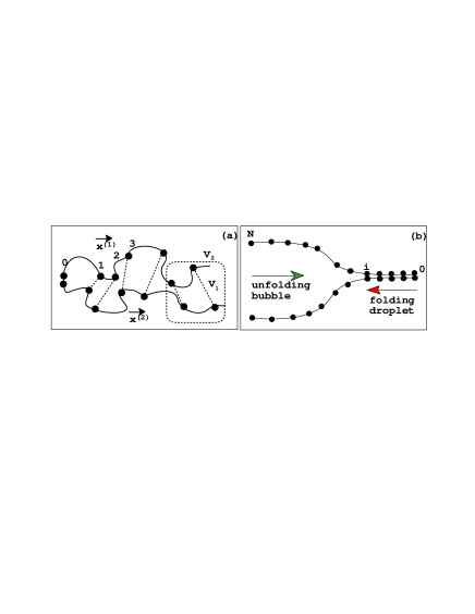
FIG. 1.: (a) A $\beta$ hairpin polymer with two interacting branches. Each branch contains $N$ residues with $\rm G\bar{o}$-like inter-chain hydrogen bond interactions ($V_{1}$, the dashed line) and with cooperative side chain packing terms ($V_{2}$, the dashed box). Here only the $\rm G\bar{o}$-interacting residues are shown. The degrees of freedom of those non-$\rm G\bar{o}$-interacting residues are assumed to be “renormalized” into those $\rm G\bar{o}$-interacting ones. (b) The hairpin zippered from the $\beta$ turn. In the folding (unfolding) regime, the droplet (bubble) will expand.

The final effects we consider arise from the (hydrophobic) side chain packing effect. This interaction depends both on the formation of inter-chain contacts and on the alignment of the local backbone [5, 9]. In principle, there are two separate pieces that one can add to our model to mimic this interaction. First, the presence of one hydrogen bond might, via the local structural dynamics (such as squeezing out water molecules), cooperatively help other neighboring residues form contacts. Such a collective term has the form $H_{\rm Sc}=-V_{2}\sum_{ij}\Delta_{i}\Delta_{j}J_{ij}$; as always, $\Delta_{i}$ indicates the contact formation of residue pair $i$, and in addition $J_{ij}$ is a coupling function indicating the range of cooperativity. The simplest short-range assumption is that $J_{ij}$ is 1 when $i,j$ are nearest-neighbors and 0 otherwise; one might also imagine a longer-ranged hierarchical side packing scheme such as that considered by Hansen et al.[10]; here we stick to the simplest possibility. This new term reflects a coupling from the primary structure to the secondary one. In addition, forming a contact limits the conformations available to the chain; in our Gaussian model, this corresponds to an increase in the chain stiffness between $i$ and $i+1$ via a term $\kappa\gamma(\Delta_{i}+\Delta_{i+1})$.

It is straightforward to integrate out the mean coordinate $\vec{X}_{i}=[\vec{x}^{(1)}+\vec{x}^{(2)}]/2$ and express the Hamiltonian in terms of the inter-residue distances only. The remaining Gaussian component will be

$$H_{\rm Gau}={\kappa\over 2}\left[\sum_{k=1}^{N}|\nabla\vec{x}_{k}|^{2}+2|\vec{x}_{0}^{(1)}-\vec{x}_{0}^{(2)}|^{2}\right]$$ (1)

Without loss of the generality, we assume that the $\beta$ turn is fixed at $\vec{x}_{0}=0$ and drop the Gaussian component $|\vec{x}_{0}^{(1)}-\vec{x}_{0}^{(2)}|^{2}$. This should not affect our result significantly if the system size is large enough. The interaction component is

$$H_{\rm int} = {\gamma\kappa\over 2}\sum_{k=2}^{N}|\nabla\vec{x}_{k}|^{2}(\Delta_{k}+\Delta_{k-1})$$ (3)

$$\hskip 2.84544pt-\sum_{k=1}^{N}\Delta_{k}\left[V_{1}+V_{2}\Delta_{k-1}\right]$$

We now proceed to find the partition function for this model. Since we are interested in the case of short-ranged $\rm G\bar{o}$ interaction, (i.e., the effective contact distance $r_{0}$ is far smaller than the thermodynamic mean inter-residue distance $1/\sqrt{\beta\kappa}$), it is reasonable to replace the Gaussian connectivity term ${\kappa\over 2}|\nabla\vec{x}_{k}|^{2}$ by ${\kappa\over 2}|\vec{x}_{k}|^{2}$ if $\vec{x}_{k-1}$ is in a contact position. This approximation will greatly simplify the calculation.

III The phase diagram

Given the above simplification, our model can be exactly solved in terms of a set of recursion relations. We are eventually interested in the full partition function, which reads

$$Z_{N}\ =\ \prod_{k=1}^{N}\int\left[{\beta\kappa\over 2\pi}\right]^{d\over 2}d^{d}x_{k}e^{-\beta H(\{\vec{x}\})}\Biggr{|}_{\vec{x}_{0}=0}$$ (4)

where $d$ is the dimensionality which we will take as 3. It will also be convenient to consider several “restricted” partition functions, corresponding to summing over all the states consistent with some extra constraints. First, we define $Z_{N,n_{f}}$ as the restricted partition function of an ensemble that contains all configurations specified by a particular number of contacts number $n_{f}$. The full partition function is just a sum of $Z_{N,n_{f}}$ over this contact number. Second, we define $Z_{N,n_{f}}^{c}$ as the restricted partition function of an ensemble specified by contact number $n_{f}$ with the polymer distal end $i=N$ being in a contact position (as indicated by the superscript “$c$”).

Finally, we introduce the partition function for a completely unfolded polymer segment running from sequence index $j$ to sequence index $i$, weighted by additional terms on the two end residues. Explicitly, the path integral of the unfolded segment takes the form

$$M_{i,j}(\mu_{1},\mu_{2}) = \prod_{k=j}^{i}\int\left[\sqrt{{\beta\kappa\over 2\pi}}\right]^{d}d^{d}x_{k}\left[1-\Delta_{k}\right]$$ (6)

$$\hskip 2.84544pt\times e^{-{\beta\kappa\over 2}\sum_{s=j+1}^{i}|\nabla\vec{x}_{s}|^{2}-{\beta\kappa\over 2\mu_{1}}|\vec{x}_{i}|^{2}-{\beta\kappa\over 2\mu_{2}}|\vec{x}_{j}|^{2}}$$

In Fig.2, we show how a variety of path integrals, which form the building blocks for the entire partition function, can be represented in terms of $M_{i,j}(\mu_{1},\mu_{2})$. This notion allows to break up the partition function into a sum of partition functions for smaller subsystems. Specifically, we have for $n_{f}>0$,

$$Z_{N,n_{f}}=Z_{N,n_{f}}^{c}+\sum_{k=n_{f}}^{N-1}M_{N,k+1}(\infty,{1\over 1+\gamma})Z_{k,n_{f}}^{c}$$ (7)

and for $n_{f}>1$,

$$Z_{N,n_{f}}^{c} = qe^{\beta V_{1}}\Biggl{\{}e^{\beta V_{2}}Z_{N-1,n_{f}-1}^{c}$$ (9)

$$\hskip 2.84544pt+\sum_{k=n_{f}-1}^{N-2}M_{N-1,k+1}({1\over 1+\gamma},{1\over 1+\gamma})Z_{k,n_{f}-1}^{c}\Biggr{\}}$$

with $q={4\pi\over 3}r_{0}^{3}\left[\sqrt{{\beta\kappa\over 2\pi}}\right]^{3}\ll 1$. These are supplemented by the boundary conditions $M_{i,j}(\mu_{1},\mu_{2})=0$ if $j>i$, $Z_{N,0}=M_{N,1}(\infty,1)$ (the coil state with $n_{f}=0$), and $Z_{N,1}^{c}=qe^{\beta V_{1}}\left[M_{N-1,1}({1\over 1+\gamma},1)+e^{\beta V_{2}}\delta_{N,1}\right]$. Note that it is straightforward to obtain $Z_{N,N}=[qe^{\beta(V_{1}+V_{2})}]^{N}$; also, $Z_{N,0}$ is always less than unity. These will be used later.

FIG. 2.: Using the $M_{i,j}(\mu_{1},\mu_{2})$ functional to represent the path integral of several diagrams. (a) For a polymer segment starting from an “open” distal end $N$ and ended at a “contact” residue $i>0$, without any residue between $N$ and $i$ being in contact position, the path integral is equal to $M_{N,i+1}(\infty,{1\over 1+\gamma})$. Here the contact energy gain from residue $i$ is not included. (b) For a polymer segment staring from the proximal end $0$ and ended at a “contact” residue $i$, without any residue between $N$ and $0$ being in contact position, the path integral reads $M_{i-1,1}({1\over 1+\gamma},1)$. (c) For polymer segment starting from one contact residue $i$ to another one $j<(i-1)$, without any residue between $i$ and $j$ being in contact position, the path integral is $M_{i-1,j+1}({1\over 1+\gamma},{1\over 1+\gamma})$. (d) For a polymer segment only containing two contiguous contact residues, the path integral reduces to 1. (e) If the entire polymer is “open”, i.e., none of the residues are in contact position, the path integral equals $M_{N,1}(\infty,1)$.

The final step of our solution involves finding a recursive formula for $M_{i,j}(\mu_{1},\mu_{2})$. Recall that we have assumed that the contact distance $r_{0}$ is far smaller than the thermodynamic inter-residue distance $1/\sqrt{\beta\kappa}$ and that therefore we can replace the Gaussian connectivity ${\beta\kappa\over 2}|\nabla\vec{x}_{k}|^{2}$ by ${\beta\kappa\over 2}|\vec{x}_{k}|^{2}$ if $\vec{x}_{k-1}$ is in contact position. If we consider a particular $i,j$ pair, we can integrate out the coordinate of the $i^{\mbox{th}}$ residue; this will yield the two terms

$$M_{i,j}(\mu_{1},\mu_{2})$$ (10)

$$\hskip 2.84544pt=\left[{\mu_{1}\over 1+\mu_{1}}\right]^{3\over 2}M_{i-1,j}(\mu_{1}+1,\mu_{2})-qM_{i-1,j}(1,\mu_{2})$$ (11)

The terms correspond to whether this residue is not or is in contact. Again, this must be supplemented by the boundary condition

$$M_{j,j}(\mu_{1},\mu_{2})=[\mu_{1}\mu_{2}/(\mu_{1}+\mu_{2})]^{3\over 2}-q$$ (12)

Using these recursion relations, we now can compute the thermodynamic probability of the native ($n_{f}=N$), unfolded coil ($n_{f}=0$), and partially folded ensembles. The partition function is dominated by the highest probability state. An all-or-none transition will occur if this dominant state changes from coil to native (as the temperature is lowered) without passing through an extended region of parameter space in which intermediate states dominate; otherwise, the transition will be continuous. Our results indicate that at a fixed value of the (cooperative stiffness increase) $\gamma$ the transition between coil and native states is 2-state-like as long as ${V_{2}\over V_{1}}$ is above some point $\rm C_{E}$. Here $\rm C_{E}$ is the triple phase coexisting point (the coil, native, and one partially folded ensembles). This is shown in fig.3(a) for the case of $\nu_{0}={4\pi\over 3}\left[{r_{0}\sqrt{\kappa}\over\sqrt{2\pi V_{1}}}\right]^{3}=.01$.

As $\gamma$ increases, the intermediate regime shrinks and eventually disappears. In other words, in order to obtain an all-or-none transition, we must have a minimal side chain packing strength $V_{2,min}$ with respect to a particular set of $V_{1}$ and $\gamma$; for large enough $\gamma$, $V_{2,min}=0$. This behavior is plotted in fig.3(b).

Although it is not relevant for the biological system, it is interesting from the general statistical physics perspective to consider what happens to the minimal $V_{2}$ as $N$ gets large. If we define the folding temperature at the point $\rm C_{E}$ as $T_{c}=1/k_{B}\beta_{c}$, then $V_{2,min}$ and $\beta_{c}$ satisfy

$$Z_{N,0}\bigr{|}_{\beta_{c}}=Z_{N,N}\bigr{|}_{\beta_{c}}=\mbox{max}\left\{Z_{N,1},Z_{N,2},\dots,Z_{N,N-1}\right\}\bigr{|}_{\beta_{c}}$$

where “$\mbox{max}\left\{x_{1},x_{2},\dots,\right\}$” picks up the maximal one in the set $\{x_{1},x_{2}\dots\}$. This leads to $Z_{N,0}|_{\beta_{c}}=Z_{N,N}|_{\beta_{c}}\geq Z_{N,N-1}|_{\beta_{c}}$. From the recursion relation (7), (9), we find that the “large $N$” components in $Z_{N,N-1}$ is $(N-2)[qe^{\beta V_{1}}]^{N-1}e^{(N-2)\beta V_{2}}M_{k,k}({1\over 1+\gamma},{1\over 1+\gamma})$ with the one-residue loop entropy $M_{k,k}$ described by eqn.(10). Combining this with the previous formula for $Z_{N,N}$, the above inequality requires

$$1 \geq q_{c}e^{\beta_{c}[V_{1}+V_{2,min}]}$$ (13)

$$\gtrsim (N-2)M_{k,k}({1\over 1+\gamma},{1\over 1+\gamma})e^{-\beta_{c}V_{2,min}}$$ (14)

with $q_{c}\approx{4\pi\over 3}r_{0}^{3}\left[\beta_{c}\kappa/2\pi\right]^{3\over 2}\ll 1$. Clearly, this implies that at large $N$ limit, the surface tension penalty (arising from $\gamma$ and $V_{2}$) must be large enough to compete with the combinatory entropy effect. At small $\gamma$, the only possible behavior consistent with the above inequality is $T_{c}\sim N^{2/3}$ and $V_{2,min}\sim N^{2/3}\ln N$. If $\gamma$ is large, it appears that there is another choice, namely the vanishing of the one-residue entropy, $M_{k,k}({1\over 1+\gamma},{1\over 1+\gamma})\sim O(1/N)$. In this case, we find that $T_{c}$ approaches a constant $k_{B}T_{c}\approx 0.83r_{0}^{2}(1+\gamma)\kappa+O(1/N)$ and $V_{2,min}\approx k_{B}T_{c}\ln[(1+\gamma)^{3/2}-1]]-V_{1}+O(1/N)$. One should note however, that in this limit our original assumption that one can approximate factors of the form $\exp{\gamma\kappa r_{0}^{2}}$ as unity is no longer accurate, and the model crosses back to the requirement of an $N$ dependent cooperative interaction.

FIG. 3.: (a): The phase diagram for a $N=100$, $\gamma=1$ $\beta$-hairpin. Here the side chain packing energy $V_{2}$ and temperature $k_{B}T$ is scaled in the unit of the hydrogen bond energy $V_{1}$. Above the point $\rm C_{E}$, the polymer has a 2-state all-or-not transition. Below $\rm C_{E}$ is the “intermediate” regime (the shadow enclosed by the dashed line) where transition might be continuous. As $\gamma$ increases, $\rm C_{E}$ decreases toward zero and the intermediate regime eventually vanishes. (b): The minimal side chain packing energy $V_{2,min}$ required for an all-or-none 2-state folding transition, on the variation of backbone stiffness modulation $\gamma$ and hairpin size $N$ ($T_{c}$ at $\rm C_{E}$ is also computed).

To summarize, we find that 2-state behavior arising from short-ranged interactions can only exist in finite size hairpin systems. For such a finite system, increasing the stiffness of the bound parts of the chain will lead to this behavior at biologically relevant values of the chain length $N$. These results are consistent with those obtained in other two-chain models [6, 11].

IV The Folding/Unfolding Rate

We now compute the unfold/folding rate for side chain packing strength $V_{2}\geq V_{2,min}$ (i.e., the parameter regime above the triple-phase point $\rm C_{E}$). The transition is 2-state-like, and the transition rate is of the Arrhenius form $k_{tx}\sim k_{0}e^{-\beta\Delta F}$, where $k_{0}$ is a kinetic prefactor (which might be different for folding versus unfolding transitions), and the exponent $\Delta F$ is the free energy difference between the saddle point configuration (the transition state structure) and the metastable state. In our system, the Arrhenius form is just the thermodynamic probability ratio between the transition ($tx$) and metastable ensembles, $Z_{tx}/Z_{meta}$; here, $Z_{meta}=Z_{N,N}$ if $T>T_{f}$, $Z_{meta}=Z_{N,0}$ if $T<T_{f}$ and $T_{f}$ is the folding temperature defined by $Z_{N,0}\bigr{|}_{T_{f}}=Z_{N,N}\bigr{|}_{T_{f}}$.

Since there are $3N$ degree of freedom in our model, in general one can expect the existence of multiple saddle point configurations. Each configuration specifies a particular “pathway” towards folding/unfolding. The saddle point configurations must be partially folded states and their contact residues could be inhomogeneously distributed. This inhomogeneity and the number of contacts in turn determine the thermodynamic probabilities of these configurations. Among them, the most likely pathway is mediated by the configuration that has the maximal thermodynamic probability. Due to the surface tension effect (arising via nonzero $\gamma$), only two particular structures need be considered, i.e., the polymer zipping from either the $\beta$ turn or the distal end. As suggested by experiment [3, 9] and by the simple logic that $\vec{x}_{0}=0$ biases the polymer towards folding, the configuration that the “folding” droplet emerges from the $\beta$ turn is the most likely one (fig.1(b)). If we define the restricted partition for this droplet (i.e., the polymer zipping from $\beta$ turn to sequence index $i$, $0<i<N$) as $Y_{i}$, from the recursive relation, we have

$$Y_{k}=\left[qe^{\beta[V_{1}+V_{2}]}\right]^{k}M_{N,k+1}(\infty,{1\over 1+\gamma})$$ (15)

The transition state, therefore, is defined as the particular state $Z_{tx}=Y_{k}$, with $Y_{k}$ satisfying $Y_{k}\leq Y_{k\pm 1}$.

FIG. 4.: (a): The Arrhenius component $\ln[Z_{tx}/Z_{meta}]$ for folding/unfolding transition and the corresponding critical droplet/bubble size on the variation of temperature. Note the “crossover” regime ($T>T_{cx}^{unfold}$ and $T<T_{cx}^{fold}$). (b): The appearance of crossover temperature $T_{cx}$ and end temperature $T_{E}$ is determined by the critical droplet/bubble size. When $T=T_{E}^{unfold}$ (the top one), $Z_{N,N}=Y_{99}$. When $T=T_{cx}^{unfold}$ (the second top one), $Y_{99}=Y_{98}$. Likewise, when $T=T_{cx}^{fold}$ (the second lowest one), $Y_{2}=Y_{1}$, and when $T=T_{E}^{fold}$ (the lowest one), $Y_{1}=Z_{N,0}$. The transition state is the lowest $\{\ln Y_{k}\}$ on every curve.

While computing the transition state, we find that for a particular set of the parameters ($V_{2}$, $V_{1}$, $\gamma$, $r_{0}$), the behavior of the folding droplet or the unfolding bubble is characterized by several temperatures: $T_{E}^{unfold/fold}$, $T_{cx}^{unfold/fold}$, and $T_{f}$ (fig.4). For $T>T_{E}^{unfold}$ (or $T<T_{E}^{fold}$), there is no transition state and the transition from native (coil) to coil (native) state is purely relaxational. Here the “end” temperature $T_{E}^{unfold}$ is defined by $Z_{N,N}\bigr{|}_{T_{E}^{unfold}}=Y_{N-1}\bigr{|}_{T_{E}^{unfold}}$, and $T_{E}^{fold}$ is defined by $Z_{N,0}\bigr{|}_{T_{E}^{fold}}=Y_{1}\bigr{|}_{T_{E}^{fold}}$. For $T_{cx}^{unfold}<T<T_{E}^{unfold}$ (or $T_{cx}^{fold}>T>T_{E}^{fold}$), on the other hand, the size of the “critical” unfolding bubble (folding droplet) is one. Here the “crossover” temperature $T_{cx}^{unfold}$ is defined by $Y_{N-2}\bigr{|}_{T_{cx}^{unfold}}=Y_{N-1}\bigr{|}_{T_{cx}^{unfold}}$, and $T_{cx}^{fold}$ is defined by $Y_{2}\bigr{|}_{T_{cx}^{fold}}=Y_{1}\bigr{|}_{T_{cx}^{fold}}$. Finally, for $T_{cx}^{fold}<T<T_{cx}^{unfold}$, the critical unfolding bubble (if $T>T_{f}$) or folding droplet (if $T<T_{f}$) has a size $k$ between 1 and $N-1$, determined by variational method, $Y_{k}\leq Y_{k\pm 1}$.

For completeness, we also computed the folding and unfolding rates based on the configuration that the droplet is initiated from the distal end instead of the $\beta$ turn. It turns out that its folding/unfolding rate is $10^{3}$-fold lower than the previous configuration. This confirms our assumption and is consistent with the experimental observation that additional inter-chain interaction near the $\beta$ turn enhances the folding rate [3, 9]. Thus we conclude that the dominant pathway for polymer folding is zippered from the $\beta$ turn; whereas the pathway for unfolding is un-zippered from the distal end.

V Discussion

We have analyzed a simple $\beta$ hairpin model and discussed the significance of side chain packing regularities. We found that side-chain packing regularities are necessary to generate 2-state transitions between coil and native structures. There will be an upper limit to the hairpin size $N$ for which this behavior persists but this does not affect its applicability to biologically relevant finite-sized chains. Since it has been shown that folding of a $\beta$-hairpin captures much of the basic physics of protein folding[3] (imagine the folding of two $\alpha$-helices connected by a $\beta$ turn; the coupling between the “secondary” and “tertiary” structure there is similar to the coupling between “primary” backbone stiffness and “secondary” contact formation here), our model can provide a fundamental understanding of how a protein can fold.

Why is the coupling induced by side chain packing important? The reason is as follows. In general, the ensemble space of a hairpin polymer contains two entropic components: one is configurational regarding local loop entropy and another is combinatory indicating the total possible arrangement of the hydrogen bonds in a partially folded state. The combinatory part grows exponentially as the system size increases, for states which have a finite fraction of the possible hydrogen bonds. This might compensate the configurational entropy loss compared to the coil state and the relatively lower hydrogen-bond energy gain compared to the native hairpin state. The partially folded state then becomes thermodynamically predominant, and the 2-state transition between coil and native states will be destroyed. To avoid this situation, a collective effect must be imposed. For the on-lattice model, this needed effect can come from the restricted arrangement of the polymer residues, since the alignment of one part of the polymer will affect the others and the influence ultimately reach the whole length of the chain [12]. On the contrary, there is no such effect in off-lattice models; instead, one has to design the Hamiltonian carefully to obtain the desired 2-state behavior.

It appears that the “side-chain packing” regularity is the essential ingredient to allow the all-or-none folding transition [3, 9, 12]; this is perhaps similar to the ideas of “hydrophobic collapse” and “non-additive” force put forth by other groups [4, 13]. The side-chain packing is essentially dependent on the “matching” of the local peptide backbone conformation and the hydrogen-bond formation [9]. We have argued that this fact leads to new cooperative terms in the Hamiltonian, as having some residues hydrogen-bonded will bias other residues to form their native contacts and also locally restrict conformational entropy. One critical consequence of this is the creation of an effective “surface tension” between the folded and unfolded regimes. This energy cost will compete with the combinatory entropy gain of a partially folded state, and the all-or-none transition can be restored. This side-chain effect is not present in systems undergoing the $\alpha$ helix-coil transition, manifesting the essential difference between $\alpha$-helix and $\beta$-hairpin formation.

Our model is, of course, greatly simplified compared to the actual $\beta$-hairpin system. One immediate criticism is that we have neglected non-native hydrogen bond formation by using the $\rm G\bar{o}$ interaction. To date, NMR evidence suggests [9] that states with non-native bonds have minimal thermodynamic weight, lending support to the adequacy of this approach. These neglected effects, however, might produce local minima in the energy landscape and trap misfolded structures, leading to a glassy molten globule.

Another problem is our use of uniform strengths for all interactions. This was necessary because of our desire to develop a recursion relationship which enables us to do calculations for reasonably high values of $N$. One can extend the model to heterogeneous couplings, but then one will have to resort to exact evaluation of each of the $2^{N}$ different states of the $\rm G\bar{o}$ contacts. This would limit us to small polymers; also, the cooperative “zippering” behavior in folding transition might be altered to start from the center of a hydrophobic cluster instead of the $\beta$ turn [4]. In any case, we do not believe that modest heterogeneity will lead to any significant changes in our results regarding the source of the cooperativity in this class of systems.

C. Guo gratefully thanks Margaret Cheung, Ralf Bundschuh $\&$ Terence Hwa for useful discussions. H. Levine acknowledges the support of the US NSF under grant DMR98-5735.

REFERENCES

- [1] Dill, K. A. Chan, HS. (1997) Nature Struct. Biol. 4, 10-19. Du, R., Pande, V. S., Grosberg, A. Yu., Tanaka, T. Shakhnovich E. S. (1998) J. Chem. Phys. 108, 334-350. Onuchic, J. N., Luthey-Schulten, Z. Wolynes, P. G. (1997) Ann. Rev. Phys. Chem. 48, 545-600. Pande. V. S., Grosberg, A. Yu., Tanaka, T. Rokhsar D. S. (1998) Curr. Opin. Struct. Biol. 8, 68-79. Wolynes, P. G., Onuchic, J. N. Thirumalai, D. (1995) Science 267, 1619-1620.
- [2] Poland, D. Scheraga, H. A. (1970) in Theory of Helix-Coil Transition in Biopolymers (Academic, New York).
- [3] Muñoz, V., Thompson, P. A., Hofrichter, J. Eaton, W. A. (1997) Nature 390, 196-199.
- [4] Klimov D. K. Thirumalai, D. (1997) Folding Design 273, 7-13. Pande, V.S. Rokhsar, D.S. (1999) Proc. Natl. Acad. Sci. USA 96, 9062-9067. Dinner, A.R., Lazaridis, T. Karplus, M. (1999) Proc. Natl. Acad. Sci. USA 96, 9068-9073.
- [5] Kilonski, A., Galazka, W. Skolnick, J. (1998) J. Chem. Phys. 108, 2608-2617.
- [6] Cule, D., Hwa, T. (1997) Phys. Rev. Lett. 79, 2375-2378.
- [7] Pande, V.S., Grosberg, A. Y. Tanaka, T. (1999) Rev. Modern Phys. (to appear).
- [8] Takada, S. Wolynes, P. G. (1997) J. Chem. Phys. 107, 9585-9598.
- [9] Muñoz, V., Henry, E. R., Hofrichter, J. Eaton, W. A. (1998) Proc. Natl. Acad. Sci. USA 95, 5872-5879.
- [10] Hansen, A., Jensen, M.H., Sneppen, K. Zocchi, G. (1998) Physica A 250, 355-361.
- [11] Dauxois, T. Peyrard, M. (1993) Phys. Rev. E 47, R44-R47; (1995) Phys. Rev. E 51, 4027-4040.
- [12] Chen, S-J. Dill, K. A. (1998) J. Chem. Phys. 109, 4602-4616.
- [13] Shoemakeer, B.A. Wolynes, P.G. (1999) J. Mol. Biol. 287, 657-656. Shoemakeer, B.A., Wang, J. Wolynes, P.G. (1999) J. Mol. Biol. 287, 675-694.