A Thermodynamic Model for Receptor Clustering

Abstract

Intracellular signaling often arises from ligand-induced oligomerization of cell surface receptors. This oligomerization or clustering process is fundamentally a cooperative behavior between near-neighbor receptor molecules; the properties of this cooperative process clearly affects the signal transduction. Recent investigations have revealed the molecular basis of receptor-receptor interactions, but a simple theoretical framework for using this data to predict cluster formation has been lacking. Here, we propose a simple, coarse-grained, phenomenological model for ligand-modulated receptor interactions and discuss its equilibrium properties via mean-field theory. The existence of a first-order transition for this model has immediate implications regarding the robustness of the cellular signaling response.

I Introduction

Cell growth, differentiation, migration, and apoptosis are in part regulated by extracellular polypeptide growth factors or cytokines (Heldin, 1995; Stuart and Jones, 1995). As these molecules are unable to pass through the hydrophobic cell membrane, they have to bind to the extracellular domains of specific surface receptors in order to exert their effects. Much effort has gone into investigating the fundamental question of how the ligand-receptor interaction can trigger the proper intracellular signals. One popular hypothesis is that ligand-induced ”clustering” of ligand-receptor complexes can be a key element in the proper activation of downstream signals. (Ashkenazi and Dixit, 1998; Bray and Levin, 1998; Heldin, 1995; Germain, 1997; Lemmon and Schlessinger, 1994, 1998; Reich et al., 1997; Sakihama et al., 1995).

As an example of this line of reasoning, we consider the signaling cascade mediated by the binding of tumor necrosis factor (TNF) to the receptor TNF-R1. Internally, the cytoplasmic domain of TNF-R1 is “sensed” by a variety of adaptor proteins, namely TRADD, FADD, TRAF2, and RIP; this sensing leads eventually to NF$-\kappa$B/JNK/SAPK activation and apoptosis. To accomplish the downstream signaling, an oligomerization of these adaptor proteins is required (Ashkenazi and Dixit, 1998). One way to facilitate oligomerization is via construction of a molecular scaffolding via TNF-induced TNF-R1 clustering. It is known that TNF-R1 will not aggregate in the absence of TNF; this is due to the association of an inhibitor, ”silencer of death domain” (SODD), which normally attaches to TNF-R1 cytoplasmic domains and prevents receptor aggregation (Jiang et al., 1999), or alternatively due to the receptor extracellular domains since spontaneous association of TNF-R1 has been observed in cells that express truncated receptors (Boldin et al., 1995; Vandevoorde et al., 1997). TNF treatment, however, can bring two or more receptors into proximity via its multiple binding capacity (Jones et al., 1990, 1992)]. This “proximity” might “squeeze” out SODD (Jiang et al., 1999), expose the cytoplasmic “death” domains to adaptor proteins, and thereby stabilize receptor clusters. Thus, a molecular scaffold/nuclei is generated to initiate signaling.

Over a longer time scale, the signaling messages can provide feedback to modify the capability of surface receptor clustering (Humphries, 1996; Wyszynski et al., 1997). This leads to a complex dynamical process involving both the intracellular signaling cascades as well as the surface receptor clustering. The self-organization made possible by these feedbacks has been intensively discussed for signaling cascades (see, e.g., Jafri and Keizer, 1995; Barkai and Leibler, 1997). Much less is understood, however, regarding the role of receptor clustering. It is clear, though, that given the hypothesis that cellular signaling relies on the formation of receptor clusters, the temporal and spatial characteristics of clustering would certainly affect the process of signaling transduction. Thus, modeling the physical properties of receptor clustering is as important as modeling signaling cascades.

Since clustering is due to an interaction between nearest-neighbor receptors, it is obviously a cooperative process. From a physics perspective a system with this type of cooperativity can exhibit a first order phase transition, corresponding to a jump in the surface density of ligand-receptor complexes. In the coexistence region of this transition, the surface will spontaneously segregate into two phases, dilute and dense. This first order phase transition endows the signal transduction process with the ability to produce a digital signal in an analog world; this is independent of the details of intracellular cascades, instead, arising from the intrinsic cooperativity in ligand-receptor interaction. This has not been adequately addressed in the few models studied to date (Goldstein and Wiegel, 1983; Goldstein and Perelson, 1984; Riley et al., 1995; Coutsias et al., 1997; Shea et al., 1997).

The purpose of this work is to introduce a phenomenological model for the TNF-TNFR1 system to describe the onset of receptor clustering (phase separation). Specifically, we assume that clustering can be described by the statistical mechanics of a simple lattice Hamiltonian, incorporating the fundamental mechanism of a multimeric binding capacity for the ligand. We will calculate (via mean-field theory) a phase diagram and show that clustering will be thermodynamically favored for some range of ligand and receptor densities. Finally, we will do a simple Monte Carlo simulation of this system, showing that receptor diffusion will lead rapidly to cluster formation in the relevant parameter range. We neglect the possibility that there exist long-time feedbacks to modify the clustering capacity, and we ignore some inessential details of the receptor-ligand interaction. More detailed models including these effects, as well as applications to other signaling systems, will be presented in the future.

II The Lattice Hamiltonian

In our model, we treat the cell surface as a lattice with a spacing of the order of a few $nm$; this is the closest that neighboring receptors can get to each other. Each lattice site $i$ has either one or zero receptor molecules, denoted as $n_{i}=$ 1 or 0. Our receptor has only two states: liganded or unliganded, and the interaction between receptor molecules is determined by their states. This ”two-state” model is over-simplified, yet we will see that it gives reasonable predictions for the phase diagram. A “state” label, $t_{i}=$ 1 or 2, to represent unliganded or liganded, then, can be assigned to each occupied receptor. We will further assume that the only ligands on the surface are those bound to receptors. If we let the chemical potential of the ligand be $\mu_{L}$ and that of the receptor be $\mu_{R}$, we then get a contribution to the effective Hamiltonian of the system

$$H_{1}(\{n,t\})=-\sum_{i}\mu(t_{i})n_{i}$$ (1)

where $\mu(1)=\mu_{R}$ and $\mu(2)=\mu_{R}+\mu_{L}+g_{L}$ and $-g_{L}$ is the binding energy between ligand and receptor.

We should clarify the relationship between the parameters used here and those in real experiments. Using standard ideas (Changeux et al., 1967), we notice that with only this term, the partition function can be factorized and reduced to a single site problem,

$$Z=\prod_{i}Z_{i}=\prod_{i}\left[1+\sum_{k=1}^{2}e^{\beta\mu(k)}\right]$$ (2)

From this, we can immediately obtain the expectation values of the TNF-R1 concentration in the liganded and unliganded states. These are assumed to correspond to the equilibrium condition of the following reaction (Corti et al., 1994; Grell et al., 1998): $\mbox{TNF-R1${}^{\rm(m)}$+TNF}\rightleftharpoons\mbox{TNF}\bullet\mbox{TNF-R1${}^{\rm(m)}$}$, with a corresponding equilibrium dissociation constant: $\frac{[{\rm TNF-R1}^{\rm(m)}]_{eq}[{\rm TNF}]}{[{\rm TNF}\bullet{\rm TNF-R1}^{\rm(m)}]_{eq}}=K_{d}^{tnf}\approx 0.59$ nM, where the notation ”TNF-R1^(m)” means TNF-R1 molecule distributed on the artificial membrane, and where the brackets [$\dots$]_eq indicates the equilibrium concentration of the respective molecule. From this, we have $e^{\beta(\mu_{L}+g_{L})}=\frac{\rm[TNF]}{K_{d}^{tnf}}$. To obtain the parameters individually, we might employ an ”ideal gas law” for the ligand. This yields $e^{\beta\mu_{L}}$=[TNF]$\left({h^{2}\over 2\pi m_{tnf}k_{B}T}\right)^{3/2}$, and $g_{L}=k_{B}T\ln\left[({2\pi m_{tnf}k_{B}T\over h^{2}})^{3/2}/K_{d}^{tnf}\right]\approx 60k_{B}T$, with $h$ as Planck constant and $m_{tnf}$ as the mass of TNF.

We next add a receptor-receptor interaction term. This takes the general form

$$H_{2}(\{n,t\})=-{1\over 2}\sum_{ij}J_{ij}a(t_{i},t_{j})n_{i}n_{j}$$ (3)

Here, $J_{ij}=1$ only when $i,j$ are nearest-neighbors and is otherwise 0 (fig.1). The function $a(t_{i},t_{j})$ indicates a “state”-dependent interaction energy between nearest-neighbor receptors, namely, $a(1,1)$ is the energy between two unliganded receptors, $a(1,2)=a(2,1)$ is the energy between one liganded and one unliganded receptors, and $a(2,2)$ is the energy between two liganded receptors. We note that in general, higher order terms might exist, especially considering the “trimeric” nature of the TNF ligand in our model problem. We have similarly neglected the details of the interactions of the ctyoplasmic domains, as per our earlier discussion. Our goal is to elucidate the basic idea regarding clustering in the simplest possible model, assured that adding more details will not change the basic notion that there exists a first-order transition due to the cooperativity.

$a(1,2)$ and $a(2,1)$ are the interaction energies, for which we will use an effective binding strength $g_{E}$ of the order of $g_{L}/10$, arising via one or two hydrogen bonds between receptors. It is important to realize that our simplified model does not treat explicitly the formation of multimers via the multimeric binding. Instead, it arbitrarily assigns the one ligand (binding two receptors into a dimer, e.g.) to one of the receptors and describes the dimeric binding as an attraction between a bound and an unbound receptor. Because of this, the model cannot distinguish between this relatively strong interaction and the subsequent much weaker interaction between the dimers. In future work, we will show that this complication does not alter the basic picture presented here.

As discussed above, in the TNF system there is probably a short-range and non-specific ”excluding” interaction between two unliganded or two liganded (with different ligand molecules) receptors. For the sake of simplicity, we will assume that the repulsive energy is of the same order of the associative one, i.e., $a(1,1)\approx a(2,2)\approx-g_{E}$. This assumption is not necessary, yet it greatly simplifies the mathematical task for analysis.

The symmetry of $a(t_{i},t_{j})$ allows us to introduce a simple matrix notation for the total Hamiltonian $H_{1}+H_{2}$. If we use two-component vectors for the state-labeling: $\tau_{i}=\left[\begin{array}[]{c}1\\ 0\end{array}\right]$ for $t_{i}=1$, and $\tau_{i}=\left[\begin{array}[]{c}0\\ 1\end{array}\right]$ for $t_{i}=2$, then the Hamiltonian can be rewritten as

$$H(\{n_{i},\tau_{i}\})=-\sum_{i}n_{i}[\mu(1),\;\mu(2)]\tau_{i}-{1\over 2}g_{E}\sum_{ij}J_{ij}n_{i}n_{j}\tau_{i}^{+}\left[\begin{array}[]{cc}-1&1\\ 1&-1\end{array}\right]\tau_{j}$$ (4)

Here $[\mu(1),\;\mu(2)]$ is an $1\times 2$ matrix. The simplicity of using this form of the matrix $a(t_{i},t_{j})$ can immediately be seen if we make a transformation $\tau_{i}={1\over 2}\left[\begin{array}[]{c}1+\sigma_{i}\\ 1-\sigma_{i}\end{array}\right]$, with $\sigma_{i}=\pm 1$. Then

$$H(\{n_{i},\sigma_{i}\})=-x\sum_{i}n_{i}-y\sum_{i}n_{i}\sigma_{i}+{1\over 2}g_{E}\sum_{ij}J_{ij}n_{i}n_{j}\sigma_{i}\sigma_{j}$$ (5)

where $x=[\mu(1)+\mu(2)]/2$ is the ”averaged” receptor chemical potential, and $y=[\mu(1)-\mu(2)]/2$ is directly related to the ligand concentration, $e^{-\beta y}=\sqrt{{[{\rm TNF}]\over K_{d}^{tnf}}}$. The partition function then reads

$$Z=\sum_{\{n_{i},\sigma_{i}\}}\exp[-\beta H(\{n,\sigma\})]$$ (6)

where $\sum_{\{n_{i};\sigma_{i}\}}$ means ensemble summation over the three different configurations $\{n_{i}=0;n_{i}=1,\sigma_{i}=\pm 1\}$ on each lattice site, $\beta=1/k_{B}T$ with $k_{B}$ as Boltzmann factor and $T$ as temperature.

If we define a new notation $u_{i}=n_{i}\sigma_{i}$, our model would be very similar to a spin-1 antiferromagnetic (AFM) BEG model (Blume et al., 1971),

$$H(\{u_{i}\})=-x\sum_{i}u_{i}^{2}-y\sum_{i}u_{i}+{1\over 2}g_{E}\sum_{ij}J_{ij}u_{i}u_{j}$$ (7)

The origin of this AFM behavior is the “negative cooperation” between nearest-neighbor receptors, as we have imposed that a “proximity” of two unliganded or two liganded receptors will cost energy. Similar behavior might occur in the erythropoietin receptor (EPO-R) and the human Growth hormone receptor (hGH-R) systems (Heldin, 1995). This negative cooperation will give rise to an absence of clustering in extreme high/low ligand concentration (i.e., $y\rightarrow\pm\infty$), and thereby result in a “bell”-shape or window-like signaling response (Elliott et al., 1996).

We should point out that this negative cooperation is not universal. In the case of EGF-R (epidermal growth factor receptor) system, a ferromagnetic (FM) behavior (“positive cooperation”) is more likely, since there clustering requires two or more liganded receptors (Lemmon et al., 1997). Thus the higher the ligand concentration, the more the EGF-R cluster can be formed, and the EGF-EGFR signaling response behaves in a sigmoidal rather than a window-like pattern. It is clear that in both EGF-R and TNF-R (and hGH-R, EPO-R) systems, the ligand multiple binding capacity is the essential ingredient to induce clustering (of course one should consider the effect from receptor cytoplasmic domain as well). Which kind of cooperation (negative or positive) one should one consider depends on the details of the receptor-receptor interaction (also including the chemical modifications on receptor cytoplasmic domains), and needs to be be established experimentally. But, the essential feature of a first-order-transition-like behavior in receptor clustering is not dependent on the sign of this additional cooperativity.

III Numerical Simulation

To see if our model can generate clustering, we perform a Monte Carlo simulation on a square lattice with the standard Metropolis scheme. For simplicity, we fix the number liganded and unliganded receptors and do not allowed these to fluctuate. Given the rather strong binding, this is not an important constraint. Furthermore, we allow motion only for individual recpetors and do not explicitly allow a clusters to move as a whole; this might not be the case in reality. The “jumping” probability for a receptor to move to another lattice site is determined by the Hamiltonian and obeys the detailed balance law. In detail, we pick a receptor at random and try to move it in a randomly chosen direction. The move is accepted if it lowers the energy and the move is accepted with probability $e^{-\beta\Delta H}$ if the energy increases.

From fig.2, we immediately see that for a given receptor density, changing the ligand concentration moves the system from a non-clustering to a clustering phase. In this figure, the open, filled circles indicate liganded, unliganded receptor molecules, respectively. Note that the open and filled circles are arranged in an alternative way to form the cluster (i.e., inside a cluster, the nearest neighbors of the open circles must be filled circles, and vice versa). This implies that the equilibrium state (which must be translationally invariant), can be described via dividing the system into two interleaved sub-lattice systems: one sub-lattice is occupied by one species of receptor molecule (liganded or unliganded), and all its nearest neighbors belong to the alternative sub-lattice which is occupied by another species.

To obtain more insight into the conditions where receptor clustering can take place, we next analyze the partition function via the mean-field approximation.

IV Mean field approximation

To proceed, we decouple the quadratic term in the Hamiltonian by introducing an auxiliary Gaussian field and employing the standard Hubbard-Stratonovich/Gaussian transformation (see, e.g., Amit, 1993; Parisi, 1988), eqn.(A3). The benefit of this transformation is to decouple the quadratic terms into linear terms such that we can sum over the ensemble configuration ($\{n_{i},\sigma_{i}\}$) at each lattice site $i$ independently. This yields (see Appendix for details)

$$Z = C\int{\cal D}\phi e^{{\beta g_{E}\over 2}\sum_{ij}J_{ij}\phi_{i}\phi_{j}+\sum_{i}S_{i}(\{\phi\})}$$ (8)

$$\mbox{with}\hskip 14.45377ptS_{i}(\{\phi\}) = \ln\left[1+2z\cosh(\beta[g_{E}\sum_{j}J_{ij}\phi_{j}+y])\right]$$ (9)

where ${\cal D}\phi=\prod_{i}d\phi_{i}$, and $C$ is a normalization constant which does not affect the thermodynamic properties of the partition function. The new field $\phi$ ranges from $-\infty$ to $+\infty$, $y=-(\mu_{L}+g_{L})/2$, and $z=e^{\beta x}=e^{\beta[\mu_{R}+(\mu_{L}+g_{L})/2]}$ is related to the receptor chemical potential which remains to be determined (in terms of the receptor density). The first term in eqn.(8) is related to the interaction energy between nearest-neighbor lattice points, whereas the second term is related to the entropy arising due to the available configurations on an individual lattice site.

In mean-field theory, we try to determine a “homogeneous” saddle point approximation for the partition function. For our system, the negative cooperation (i.e. the AFM nature) suggests that the system might prefer having neighboring sites in oppositely liganded states. Thus, we separate the lattice into two interleaved sub-lattice systems: all nearest-neighbors of a lattice site belong to the alternate sub-lattice (fig.1). We then assign two “uniform” order parameters, $\phi_{\pm}$ to each sublattice. After this assumption, the exponent of the Boltzmann factor in the partition function [eqn.(8)] now becomes $\rightarrow{\rm{N\over 2}}\left[\beta g_{E}D\phi_{+}\phi_{-}+S(\phi_{+},\phi_{-})\right]$, where N is the number of total lattice sites, $S(\phi_{+},\phi_{-})=\sum_{k=\pm}\ln[1+2z\cosh(\beta[g_{E}D\phi_{k}+y])]$, and $D$ is the number of nearest neighbors, which depends on the structure of lattice. For instance, a square lattice yields $D=4$, whereas a honeycomb lattice yields $D=3$.

Next, we minimize the free energy by varying $\phi_{\pm}$. The variation yields the “saddle point” equation

$$\left\{{\partial\over\partial\phi_{\pm}}\Bigl{[}\beta g_{E}D\phi_{+}\phi_{-}+S(\phi_{+},\phi_{-})\Bigr{]}\Bigl{|}_{\phi_{\pm}=\widetilde{\phi}_{\pm}}\right\}=0$$

. Working this out explicitly, we find a self-consistent equation for $\widetilde{\phi}_{\pm}$

$$\widetilde{\phi}_{\pm}=-\frac{2z\sinh[\beta(g_{E}D\phi_{\mp}+y)]}{1+2z\cosh[\beta(g_{E}D\phi_{\mp}+y)]}$$ (10)

with the free energy density

$$f(\widetilde{\phi}_{+},\widetilde{\phi}_{-},z)=-{g_{E}D\over 2}\widetilde{\phi}_{+}\widetilde{\phi}_{-}-{k_{B}T\over 2}\sum_{k=\pm}\ln[1+2z\cosh(\beta[g_{E}D\widetilde{\phi}_{k}+y])]$$ (11)

Finally, the mean-field receptor density is given by $\langle n\rangle=-\partial f(\widetilde{\phi}_{+},\widetilde{\phi}_{-},z)/\partial\mu_{R}$. Explicitly, we have

$$\langle n\rangle\ =\ \sum_{k=\pm}\frac{z\cosh(\beta[g_{E}D\widetilde{\phi}_{k}+y])}{1+2z\cosh(\beta[g_{E}D\widetilde{\phi}_{k}+y])}$$ (12)

We can therefore determine the receptor chemical potential, $x$ (or equivalently $z$) in terms of $\langle n\rangle$. Thereafter, we can rewrite the free energy density in terms of $\langle n\rangle$, $\widetilde{\phi}_{+}$, and $\widetilde{\phi}_{-}$.

V The onset of clustering

There is no closed form solution for eqn.(10). To get some analytical information, we define $\widetilde{\phi}_{\pm}=m\pm\epsilon$ and, with $U(w)=\frac{2z\sinh[\beta(g_{E}Dw+y)]}{1+2z\cosh[\beta(g_{E}Dw+y)]}$, we have

$$m=-\sum_{k=0}^{\infty}\frac{\epsilon^{2k}}{(2k)!}U^{(2k)}(m)$$ (13)

$$\epsilon=\sum_{k=0}^{\infty}\frac{\epsilon^{2k+1}}{(2k+1)!}U^{(2k+1)}(m)$$ (14)

where $U^{(k)}(w)=d^{k}U(w)/dw^{k}$. The basic idea of separating out the $\epsilon$ dependence is that solutions with non-zero values of $\epsilon$ represent phases in which the proximity of neighboring receptors gives rise to alternating ligand binding. For very small receptor densities, there are few neighboring receptors and hence we expect to find a unique solution of the mean-field equations with $\epsilon=0$. In fact, it is clear from eqn. (14) that there is a solution with $\epsilon=0$ for all values of the parameters, but at larger densities, there may be other more stable phases. The goal of our analysis will be to understand the general structure of the phase diagram and then to obtain more quantitative detail by numerical means.

To proceed, let us assume that $\epsilon$ is small and solve eqns.(13), (14) to order $\epsilon^{2}$;

$$m = m_{0}-m_{1}\epsilon^{2}$$ (15)

$$\mbox{with}\;\;m_{0} = -U^{(0)}(m_{0})$$ (16)

$$m_{1} = \frac{U^{(2)}(m_{0})}{2!\left[1+U^{(1)}(m_{0})\right]}$$ (17)

$$\epsilon^{3}=\frac{\left\{U^{(1)}(m_{0})-1\right\}\epsilon}{m_{1}U^{(2)}(m_{0})-\frac{1}{6}U^{(3)}(m_{0})}$$ (18)

Using the relationship given above for $\langle n\rangle$, It is easy to verify that $U^{(1)}(m_{0})=\beta g_{E}D[\langle n\rangle-m_{0}^{2}]$, $U^{(2)}(m_{0})=-m_{0}(\beta g_{E}D)^{2}[1-3\langle n\rangle+2m_{0}^{2}]$, and

$$U^{(3)}(m_{0})=\left(\left[1-3\langle n\rangle+6m_{0}^{2}\right]\left[\langle n\rangle-m_{0}^{2}\right]-3m_{0}^{2}\left[1-\langle n\rangle\right]\right)\ \left(\beta g_{E}D\right)^{3}$$

We must consider separately the cases where the denominator of eqn. (18) is positive or negative. Let us first imagine it is positive, Then, the existence of a non-trivial solution of eqn. (18) requires that $\left\{\beta g_{E}D[\langle n\rangle-m_{0}^{2}]-1\right\}>0$. At small $\langle n\rangle$ this condition will clearly fail and we will have only the trivial solution. Also, this condition will fail at $\langle n\rangle$ close to 1 for large enough $|y|$. We can see this by comparing the equation for $m_{0}$ with the expression for $\langle n\rangle$. Note that if $y$ is large enough such that the hyperbolic functions can be replaced by exponentials, we have $|m_{0}|=\langle n\rangle$, and the above expression can be replaced by $\left\{\beta g_{E}D[\langle n\rangle-\langle n\rangle^{2}]-1\right\}$; this is negative for the stated condition. As we cross a line in parameter space such that this factor changes sign to positive, there will be new solutions at non-zero $\epsilon^{2}$ and the one at $\epsilon=0$ becomes a local maximum of the free energy. This emergence of a double-well structure, with a continuous growth the non-zero $\epsilon^{2}$ solution indicates that the system exhibits a second-order phase transition.

We must next take into account the possibility that $\left\{m_{1}U^{(2)}(m_{0})-\frac{1}{6}U^{(3)}(m_{0})\right\}<0$. Having the denominator cross zero gives rise in our current approximation to a large value of $\epsilon$ which thus invalidates the neglect of higher-order terms. Typically, the higher-order terms will stabilize the system at some finite value of $\epsilon$, which thus appears “spontaneously” as some parameter threshold is crossed. This is a first-order phase transition, or equivalently a triple-well structure for the free energy. If the local minima (for zero and non-zero $\epsilon^{2}$) have equally low free energy density, the system can exist in a mixture of the two phases. As we will see, the two coexisting phases differ in their receptor density. Finally, the points where both $\left\{\beta g_{E}D[\langle n\rangle-m_{0}^{2}-1]=0\right\}$ and $\left\{m_{1}U^{(2)}(m_{0})-\frac{1}{6}U^{(3)}(m_{0})\right\}=0$, are “critical end-points” points, since they correspond to places where a second-order transition line ends at a first-order line. A diagram of this behavior, generated by the numerical solution of the mean-field equations, is given in fig. 3.

For a given ligand concentration, we can find the phase coexistence lines arising due to the first-order phase transition. This is done by finding two solutions (solved with differing values of $\epsilon^{2}$) of the mean field equations and then fixing $z$ (as a function of $y$) by requiring that they have equal free-energy

$$f(\phi^{(d)},\phi^{(d)},z)=f(\phi_{-}^{(c)},\phi_{+}^{(c)},z)$$ (19)

where $\phi_{\pm}^{(c)}$, are the order parameters for the dense condensed phase and $\phi^{(d)}$ the (equal) ones for the dilute phase. For the condensed phase, the receptor density is close to unity for reasonable values of the cooperativity parameter $\beta g_{E}D$. The workings of this system as far as signaling is concerned is shown in fig. 4. Assume there is some fixed value of the receptor density. As the ligand concentration is increased, we will cross the phase transition boundary and the receptors will segregate into a condensed phase and a dilute one, corresponding to the two co-existing mean-field solutions. Under our basic hypothesis that signaling is effected by having dense clusters, the response will exhibit a sharp jump at a specific threshold ligand concentration. Similarly, as the ligand concentration becomes too high we cross back to the uniform receptor density state and signaling ceases. That is, we have a ligand concentration “window” for receptor clustering.

As can seen from the figure, the “clustering” window will cease to exist below some minimal receptor density, as we never enter the phase coexistence region. By symmetry, this minimal density can be found by solving the mean field equations for $y=0$ where $m=0$. This leads after some algebra to the self-consistent equations

$$\langle n\rangle_{min}^{(d)} = \frac{e^{\beta g_{E}D\epsilon^{2}/2}-1}{\cosh[\beta g_{E}D\epsilon]-1}$$ (20)

$$\mbox{with}\;\epsilon = \langle n\rangle_{min}^{(d)}\tanh[\beta g_{E}D\epsilon]$$ (21)

The numerical solution of these equations is presented in fig.5. As the cooperativity parameter is increased, the minimum density which will support a clustering window goes rapidly to zero. For the TNF-TNFR1 cluster, it has been speculated that the structure of cluster is a honeycomb-like lattice (Bazzoni and Beutler, 1995; Naismith et al., 1995, 1996), which implies the number of nearest-neighbor $D=3$. If we use our rough estimate $g_{E}\simeq g_{L}/10\simeq 6kT$, we find that $\langle n\rangle_{min}^{(d)}\lesssim 10^{-6}/a_{0}^{2}$. Here $a_{0}$ is length scale of the lattice spacing. If we take $a_{0}\approx 1$ nm, on a cell with surface area 100$\mu m^{2}$, this estimate yields a requirement for less than $10^{2}$ TNF-R1 molecule distributed on the cell surface. Given that an average number of expressed TNF-R1 on cell surface is $\sim 2000$, we find that the cell operates within the desired part of the phase diagram and hence should exhibit strong sensitivity to the application of TNF. However, we should point out that this estimate is very rough, as we have made a number of simplifying assumptions and this issue needs to be re-visited with a more precise model of the receptor interactions.

VI Discussion

We have presented a simple model for signal transduction via receptor clustering, based loosely on the TNF-TNFR1 system. Our basic idea is simple. The interaction between receptors can lead to a first-order phase transition with a discontinuous jump in the receptor density as a function of the receptor chemical potential and/or the ligand concentration. Turning this around, this implies that the receptor system will spontaneously phase separate for a range of ligand concentrations. This fact about the thermodynamic equilibrium state will lead under reasonable kinetic assumptions to the rapid formation of receptor clusters. Assuming that these clusters are necessary for the signal to proceed downstream has the immediate consequence that the system exhibits a strong robust response independent of any details of the intracellular signaling cascade. This might provide a simple solution to the problem faced by biological evolution of how to get digital response in an analog world.

From a physics perspective, there is nothing very surprising about our phase diagram findings. The idea of a ”lattice” Hamiltonian with intrinsic ”cooperativity” has been proposed before (Changeux et al., 1967), and on general grounds models of this sort can be expected to have first order phase transitions. What is new here is the connection of the transition to signaling via the idea of receptor clustering. This connects nicely with increasing evidence that clustering is “universal” among many types of receptor classes.

In our model, we have ignored more-than-two receptor interaction, and relevant internal chemical degrees of freedom (such as the dissociation of SODD in the TNF-R1 system). We do not expect these detailed considerations to change the overall picture, but a more sophisticated model will be needed to make more quantitative estimates of ligand thresholds, cluster structures and most interestingly, clustering dynamics. We hope to report on these issues in the future, as well as on the extension of our models to other ligand-receptor systems.

Finally, it would be important to extend our work to later-stage dynamics, as that would allow the consideration of processes such as adaptor protein-mediated receptor internalization, cytoskeleton-assisted cluster stabilization, receptor affinity regulation, receptor cross talk, and adaptation (Barkai and Leibler, 1997; Hahn et al., 1993; Humphries et al., 1996; Holsinger et al., 1998; Luo and Lodish, 1997; Stewart et al., 1998; Sundberg and Rubin, 1996; Valitutti et al., 1995; Wyszynski et al., 1997). Other possible extensions might involve the inclusion of spatial fluctuations, the explicit treatment of external perturbations (Shoyab and Todaro, 1981), the local heterogeneity of the micro-environment (Bean et al., 1988; Ward and Hammer, 1992), or fluctuations of ligand concentration; all of these issues have been neglected here.

VII acknowledgment

Chinlin Guo wishes to acknowledge the LJIS Interdisciplinary Training Program and the Burroughs Wellcome Fund for fellowship support. He also acknowledges Margaret Cheung for the help with the numerical simulation. Herbert Levine acknowledges the support of the US NSF under grant DMR98-5735.

A The Gaussian Transformation

The identity

$$\int_{-\infty}^{\infty}dx\exp\left[-{1\over 2g}x^{2}+isx\right]=C\times\exp\left[-{g\over 2}s^{2}\right]$$ (A1)

with $g>0$, $i=\sqrt{-1}$, and $C$ as some constant, can be generalized to

$$\int_{-\infty}^{\infty}\prod_{i}dx_{i}\exp\left[-{g\over 2}\sum_{jk}x_{j}J_{jk}x_{k}+ig\sum_{j}s_{j}\sum_{k}J_{jk}x_{k}\right]=C\times\exp\left[-{g\over 2}\sum_{ij}s_{i}J_{ij}s_{j}\right]$$ (A2)

as long as $J$ is a symmetric positive definite matrix. Thus, eqn.(8) can be obtained by

$$Z = \sum_{\{n_{i},\sigma_{i}\}}\exp\left\{\beta[x\sum_{i}n_{i}+y\sum_{i}n_{i}\sigma_{i}-{g_{E}\over 2}\sum_{ij}J_{ij}n_{i}\sigma_{i}n_{j}\sigma_{j}]\right\}$$ (A3)

$$= \sum_{\{n_{i},\sigma_{i}\}}C_{\theta}\int\prod_{j}\theta_{j}e^{-{\beta g_{E}\over 2}\sum_{jk}J_{jk}\theta_{j}\theta_{k}+\sum_{j}\beta[x+\sigma_{j}(y+ig_{E}\sum_{k}J_{jk}\theta_{k})]n_{j}}$$ (A4)

$$= C_{\phi}\int\prod_{j}\phi_{j}e^{{\beta g_{E}\over 2}\sum_{jk}J_{jk}\phi_{j}\phi_{k}}\times\left\{\sum_{\{n_{j},\sigma_{j}\}}e^{\sum_{j}\beta[x+\sigma_{j}(y+g_{E}\sum_{k}J_{jk}\phi_{k})]n_{j}}\right\}$$ (A5)

$$= C_{\phi}\int\prod_{j}\phi_{j}e^{{\beta g_{E}\over 2}\sum_{jk}J_{jk}\phi_{j}\phi_{k}}\times\prod_{j}\left\{\sum_{n_{j},\sigma_{j}}e^{\beta[x+\sigma_{j}(y+g_{E}\sum_{k}J_{jk}\phi_{k})]n_{j}}\right\}$$ (A6)

$$= C_{\phi}\int\prod_{j}\phi_{j}e^{{\beta g_{E}\over 2}\sum_{jk}J_{jk}\phi_{j}\phi_{k}}\times\prod_{j}\left\{1+2z\cosh\Biggl{[}\beta\Bigl{(}g_{E}\sum_{k}J_{jk}\phi_{k}+y\Bigr{)}\Biggr{]}\right\}$$ (A7)

$$= C_{\phi}\int\prod_{j}\phi_{j}e^{{\beta g_{E}\over 2}\sum_{jk}J_{jk}\phi_{j}\phi_{k}+\sum_{j}S_{j}(\{\phi\})}$$ (A8)

where $i=\sqrt{-1}$, $\phi_{k}=i\theta_{k}$, $S_{j}(\{\phi\})=\ln\left[1+2z\cosh(\beta[g_{E}\sum_{k}J_{jk}\phi_{k}+y])\right]$, and $C_{\theta}$, $C_{\phi}$ are integral constants.

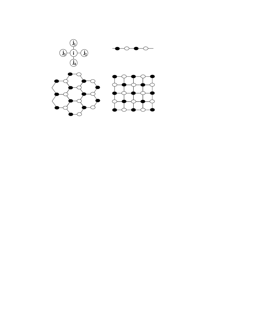
FIG. 1.: Interleaved sublattices labeled as filled/open circles on one dimensional, and two dimensional (square/honeycomb) space. On a square lattice, $j_{1,2,3,4}$ is the nearest neighbors to site $i$.

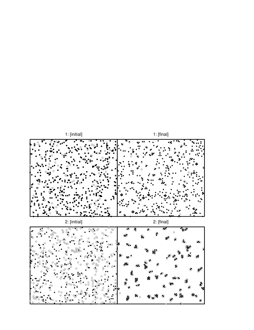
FIG. 2.: Monte Carlo simulation with Metropolis scheme. Here we test the model under a fixed receptor density but different ligand concentrations. In both upper and lower panels, the left figure represent initial conditions and the right are results after $10^{8}$ Monte Carlo steps. The open, filled circles indicate liganded, unliganded receptor molecules, respectively. There is no stable cluster formation in the upper snapshot, whereas the clustering is stable in the lower one. Here we use $g_{E}=6k_{B}T$, density of liganded receptor: upper plane, 0.001, lower plane, 0.03, and density of unliganded receptor: upper plane, 0.059, lower plane, 0.03.

FIG. 3.: Numerically computed phase diagram, showing that there is a pair of second-order lines each of which ends on the first-order transition curve. (C=critical point; $\rm C_{E}$=critical endpoint). The phase to the lower-right has $\epsilon\neq 0$. Here we used $g_{E}=6k_{B}T$ and $D=3$. To show the symmetry, we plot the ligand concentration in logarithm unit, normalized with respect to the dissociation constant $K_{d}^{tnf}=0.59$ nM. Here the chemical potential $\mu_{R}$ is related to receptor density. In fig. 4, we convert the receptor chemical potential into the molecular density.

FIG. 4.: The phase diagram now shown as a function of the receptor density $\langle n\rangle$ related to the ligand concentration. To show the symmetry, we plot the ligand concentration in logarithm unit, normalized with respect to the dissociation constant $K_{d}^{tnf}=0.59$ nM. The region inside the solid lines is the co-existence region where states of high and low density co-exist. As the ligand concentration is altered so as to cross one of these lines, the receptors will spontaneously cluster and thereby allow signaling to occur. $\langle n\rangle_{min}^{(d)}$ is the minimal receptor density for clustering. For this set of parameters, clustering will occur even for very small overall receptor density. Here $a_{0}$ is the length scale for the lattice spacing. For surface receptor molecule such as TNF-R1, we might take $a_{0}\approx 1$ nm.

FIG. 5.: The variation of $\langle n\rangle_{min}^{(d)}$ as a function of the association energy $g_{E}$. We find that $\langle n\rangle_{min}^{(d)}$ rapidly approaches zero once $g_{E}D\geq 15k_{B}T$. If we assign $D=3\sim 4$, this energy scale corresponds to a single hydrogen bond. Here $a_{0}$ is the length scale for the lattice spacing. For a surface receptor molecule such as TNF-R1, we might take $a_{0}\approx 1$ nm.

REFERENCES

- [1] Amit, D. J. 1993. Field theory, the renormalization group, and critical phenomena. World Scientific pub. New Jersey.
- [2] Ashkenazi, A; Dixit, VM. Death receptor: 1998. Signaling and modulation. Science. 281:1305-1308.
- [3] Barkai, N; Leibler, S. 1997. Robustness in simple biochemical networks Nature. 387:913-917.
- [4] Bray, D; Levin, MD; Morton-Firth, CJ. 1998. Receptor clustering as a cellular mechanism to control sensitivity Nature. 393:85-88.
- [5] Bazzoni, F; Beutler, B. 1995. How do tumor necrosis factor receptors work? J. Inflamm.. 45:221-238.
- [6] Bean, JW; Sargent, DF; Schwyzer, R. 1988. Ligand/receptor interactions–the influence of the microenvironment on macroscopic properties. Electrostatic interactions with the membrane phase. J. Recep. Res. 8:375-389.
- [7] Blume, M.; Emery, V.J.; Griffiths, R.B. 1971. Ising model for the transition and phase separation in mixtures. Phys. Rev. A. 4:1071-1077.
- [8] Boldin, MP; Mett, IL; Varfolomeev, EE; Chumakov, I; Shemer-Avni, Y; Camonis, JH; Wallach, D. 1995. Self-association of the ”death domains” of the p55 tumor necrosis factor (TNF) receptor and Fas/APO1 prompts signaling for TNF and Fas/APO1 effects. J. Biol. Chem. 270:387-391.
- [9] Changeux, J-P; Thiery, J; Tung, Y; Kittel C. 1967. On the cooperativity of biological membranes. Proc. Natl. Acad. Sci. USA. 57:335-341.
- [10] Corti, A; Poiesi, C; Merli, S; Cassani, G. 1994. Tumor necrosis factor (TNF)α quantification by ELISA and bioassay: effects of TNFα-soluble TNF receptor (p55) complex dissociation during assay incubations. J. Immunol. Methods. 177:191-198.
- [11] Coutsias, E.A.; Wester, M.J.; Perelson, A.S. 1997. A nucleation theory of cell surface capping. J. Statist. Phys. 87:1179-1203.
- [12] Elliott, S; Lorenzini, T; Yanagihara, D; Chang, D; Elliott, G. 1996. Activation of the erythropoietin (EPO) receptor by bivalent anti-EPO receptor antibodies. J. Biol. Chem. 271:24691-24697.
- [13] Germain, RN. 1997. T-cell signaling: the importance of receptor clustering. Curr. Biol. 7:R640-R644.
- [14] Goldstein, B; Perelson, AS. 1984. Equilibrium theory for the clustering of bivalent cell surface receptors by trivalent ligands. Application to histamine release from basophils. Biophys. J. 45:1109-1123. Goldstein, B; Wiegel, FW. 1983. The effect of receptor clustering on diffusion-limited forward rate constants. Biophys. J. 43:121-125.
- [15] Grell, M; Wajant, H; Zimmermann, G; Scheurich, P. 1998. The type 1 receptor (CD120a) is the high-affinity receptor for soluble tumor necrosis factor. Proc. Natl. Acad. Sci. USA. 95:570-575.
- [16] Hahn, WC; Burakoff, SJ; Bierer, BE. 1993. Signal transduction pathways involved in T cell receptor-induced regulation of CD2 avidity for CD58. J. Immunol. 150:2607-2619.
- [17] Heldin, Carl-Henrik. 1995. Dimerization of cell surface receptors in signal transduction. Cell. 80:213-223.
- [18] Humphries MJ. 1996. Integrin activation: the link between ligand binding and signal transduction. Curr. Opin. Cell. Biol.. 8:632-640.
- [19] Holsinger, LJ; Graef, IA; Swat, W; Chi, T; Bautista, DM; Davidson, L; Lewis, RS; Alt, FW; Crabtree, GR. 1998. Defects in actin-cap formation in Vav-deficient mice implicate an actin requirement for lymphocyte signal transduction. Curr. Biol. 8:563-572.
- [20] Jafri, MS; Keizer, J. 1995. On the roles of diffusion, buffers, and the endoplasmic reticulum in IP3-induced waves. Biophys. J. 69:2139-2153.
- [21] Jiang, Y; Woronicz, JD; Liu, W; Goeddel, DV. 1999. Prevention of constitutive TNF receptor 1 signaling by silencer of death domains. Science. 283:543-546.
- [22] Jones, EY; Stuart, DI; Walker, NP. 1990. The structure of tumour necrosis factor–implications for biological function. J. Cell Sci. 13:11-8. Jones, EY; Stuart, DI; Walker, NP. 1992. Crystal structure of TNF. Immunol. Series. 56:93-127.
- [23] Lemmon, MA; Bu, Z; Ladbury, JE; Zhou, M; Pinchasi, D; Lax, I; Engelman, DM; Schlessinger, J. 1997. Two EGF molecules contribute additively to stabilization of the EGFR dimer. Embo J. 16:281-294. Lemmon, MA; Schlessinger, J. 1994. Regulation of signal transduction and signal diversity by receptor oligomerization. Trends Biochem. Sci. 19:459-463. 1998. Transmembrane signaling by receptor oligomerization. Methods Mol. Biol. 84:49-71.
- [24] Luo, K; Lodish, HF. 1997. Positive and negative regulation of type II TGF-beta receptor signal transduction by autophosphorylation on multiple serine residues. Embo. J. 16:1970-1981.
- [25] Naismith, JH; Brandhuber, BJ; Devine, TQ; Sprang, SR. 1996. Seeing double: crystal structures of the type I TNF receptor. J. Mol. Recogn. 9:113-117. Naismith, JH; Devine, TQ; Brandhuber, BJ; Sprang, SR. 1995. Crystallographic evidence for dimerization of unliganded tumor necrosis factor receptor. J. Biol. Chem. 270:13303-13307.
- [26] Parisi, G. 1988. Statistical Field Theory. Addison Wesley Pub. California.
- [27] Reich, Z; Boniface, JJ; Lyons, DS; Borochov, N; Wachtel, EJ; Davis, MM. 1997. Ligand-specific oligomerization of T-cell receptor molecules. Nature. 387:617-620.
- [28] Riley, M.R.; Buettner, H.M.; Muzzio, F.J.; Reyes, S.C. 1995. Monte Carlo simulation of diffusion and reaction in two-dimensional cell structures. Biophys. J. 68:1716-1726.
- [29] Sakihama, T; Smolyar, A; Reinherz, EL. 1995. Molecular recognition of antigen involves lattice formation between CD4, MHC class II and TCR molecules. Immunol. Today. 16:581-587.
- [30] Shea, L.D.; Omann, G.M.; Linderman, J.J. 1997. Calculation of diffusion-limited kinetics for the reactions in collision coupling and receptor cross-linking. Biophys. J. 73:2949-2959.
- [31] Shoyab, M; Todaro, GJ. 1981. Perturbation of membrane phospholipids alters the interaction between epidermal growth factor and its membrane receptors. Archv. Biochem. Biophys. 206:222-226.
- [32] Stewart, MP; McDowall, A; Hogg, N. 1998. LFA-1-mediated adhesion is regulated by cytoskeletal restraint and by a -dependent protease, calpain. J. Cell Biol. 140:699-707.
- [33] Stuart, DI; Jones, EY. 1995 Recognition at the cell surface: recent structural insights. Curr. Opin. Struct. Biol. 5:735-743.
- [34] Sundberg, C; Rubin, K. 1996. Stimulation of integrins on fibroblasts induces PDGF independent tyrosine phosphorylation of PDGF -receptors. J. Cell Biol. 132:741-752.
- [35] Valitutti, S; Dessing, M; Aktories, K; Gallati, H; Lanzavecchia, A. 1995. Sustained signaling leading to T cell activation results from prolonged T cell receptor occupancy. Role of T cell actin cytoskeleton. J. Exp. Med. 181:577-584.
- [36] Vandevoorde, V; Haegeman, G; Fiers, W. 1997. Induced expression of trimerized intracellular domains of the human tumor necrosis factor (TNF) p55 receptor elicits TNF effects. J. Cell Biol. 137:1627-16238.
- [37] Ward, MD; Hammer, DA. 1992. Morphology of cell-substratum adhesion. Influence of receptor heterogeneity and nonspecific forces. Cell Biophys. 20:177-222.
- [38] Wyszynski, M; Lin, J; Rao, A; Nigh, E; Beggs, AH; Craig, AM; Sheng,M. 1997. Competitive binding of -actinin and calmodulin to the NMDA receptor. Nature. 385:439-442.