[

Inversion Symmetry and Critical Exponents of Dissipating Waves in the Sandpile Model

Abstract

Statistics of waves of topplings in the sandpile model is analyzed both analytically and numerically. It is shown that the probability distribution of dissipating waves of topplings that touch the boundary of the system obeys the power-law with critical exponent $5/8$. This exponent is not independent and is related to the well-known exponent of the probability distribution of last waves $11/8$ by exact inversion symmetry $s\to 1/s$. Probability distribution of those dissipating waves that are also last in an avalanche is invariant under the inversion transformation and has asymptotic behavior $s^{-1}$. Our extensive numerical simulations not only support these predictions, but also indicate that inversion symmetry is also useful for the analysis of the two-wave probability distributions.

]

The concept of self-organized criticality (SOC) introduced by Bak, Tang and Wiesenfeld [1] is considered to be the underlying cause of a variety of critical phenomena involving dissipative, nonlinear transport in open systems. In these phenomena a system with infinite number of degrees of freedom, when driven by external random force, evolves stochastically into a certain critical state on which it exhibits properties similar to that of a second order phase transitions. This critical state is characterized by strong fluctuations of the order parameter with power-law decay of correlation functions and absence of any characteristic length or time scale. However, unlike second order phase transitions, in the SOC phenomena the criticality emerges automatically without fine tuning of any parameters like temperature or pressure. Kolmogorov theory of isotropic and homogeneous turbulence [2] and the theory of fractal growth proposed by Kardar, Parisi and Zhang [3] are probably the most important physical examples of SOC.

To illustrate the basic ideas of SOC Bak, Tang and Wiesenfeld introduced a cellular automaton now commonly known as sandpile model because of the crude analogy between its dynamical rules and the way sand topples when building a real pile of sand. One natural formulation of the sandpile model is given in terms of integer height variables $z_{i}$ at each site of a planar square lattice ${\cal L}$. In a stable configuration the height $z_{i}$ at any site $i\in{\cal L}$ takes values $1,2,3$ or $4$. Particles are added at randomly chosen sites and the addition of a particle increases the height at that site by one. If this height exceeds the critical value $z_{c}=4$, then the site topples, and on toppling its height decreases by $4$ and the heights at each of its neighbors $j$ increases by $1$. These neighboring sites may become unstable in their turn and the toppling process continues causing an avalanche.

Extensive numerical simulations of this simple model verified that it captures all the essential features of SOC [4]. Another reason why a lot of attention has been attracted to this model during last years is that the problem admits a purely analytic treatment. Dhar [5] discovered the Abelian structure of the sandpile dynamics and then Dhar and Majumdar [7] proved that recurrent sandpile configurations are in one-to-one correspondence with the spanning trees on the lattice. This result gave a key to exact calculation of height probabilities in the bulk of the lattice [6, 8] and height-height correlation functions at the boundary [9].

All these advances notwithstanding, the derivation of the probability distribution of avalanches still remains an important open problem. Recent numerical simulations [10] indicate that this probability distribution is actually multi-fractal. The avalanches propagating up to the boundary and, hence, dissipating particles there seem to form very special subclass of avalanches which obey pure scaling. This is the reason why the analysis of dissipating events becomes of especial importance. It is the aim of the Letter to clarify the issue and to study the probability distributions of some classes of dissipating events.

The spanning trees representation turned out to be very useful not only in the study of static height-height correlations but also in the analysis of the avalanche process. Namely, every avalanche may be represented as a sequence of more elementary events, so-called waves of topplings. These can be organized as follows [11]: if the site $i$ to which a grain was added becomes unstable, topple it once and then topple all other sites of the lattice that become unstable, keeping the initial site $i$ from second toppling. The set of sites toppled thus far is called the first wave of topplings. After the first wave is completed the site $i$ is allowed to topple the second time, not permitting it to topple again until the second wave of topplings is finished. The process continues until the site $i$ becomes stable and the avalanche stops.

Waves of topplings being more elementary events than avalanches have also much simpler properties. First, each site involved into a wave topples exactly once in that wave. As a result, the height profile of the system after a wave is exactly the same as before the wave except at sites on the single closed boundary of the wave which separates sites that toppled in that wave from those that did not. Just inside the wave boundary a trough (relative to the previous heights) appears , whereas outside the boundary a hill appears where sand was moved out of the wave boundary. The avalanche can stop only if the site where avalanche was initiated has at least one neighboring site not belonging to the last wave and therefore the very last wave in the avalanche should touch the origin of the avalanche. All the waves are individually compact, so, we shall characterize the waves of topplings only by their area.

The most important of geometrical properties of waves is the one-to-one correspondence between waves and two-component spanning trees where one component corresponds to the wave itself and the other to the rest of the lattice.

The expected number of different waves of topplings is related to the Green function of the Laplacian operator and was found to be [9]

$$W_{all}(s)~{}{\rm d}s\sim\frac{{\rm d}s}{s}.$$ (1)

Note that the distribution function ${\rm Prob}[s>s_{0}]$ of all waves is logarithmically divergent both on the ultraviolet cutoff $a$ (step of the lattice) and infrared cutoff $L$ (lattice size).

This probability distribution is obviously invariant under the inversion transformation $r\to R^{2}/r$, where $R=\sqrt{aL}$ is called an inversion radius. The meaning of this transformation can easily been understood as follows. Let us consider stereographic projection from the plane to the sphere as shown on Fig.1.

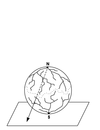
FIG. 1.: Stereographic projection from plane onto sphere transforms the spanning tree so that one its component is attached to the south pole of the sphere, and another to the north.

The boundary of the system in such a projection is mapped to the north pole while the point where a wave of topplings was initiated to the south pole. Two-component spanning tree on the plane that represents the height configuration after a given wave of topplings will be transformed into the similar tree on the sphere. Its one component is attached to north pole of the sphere and the other component to the south pole. Both poles of the sphere are formally equivalent and inversion transformation interchanges them.

Inversion transformation is only one of the family of conformal symmetries. Inversion, however, is of special importance for us since it provide us with information about the distribution of dissipating waves of topplings, i.e. those waves that touch the boundary of the system and dissipate particles there.

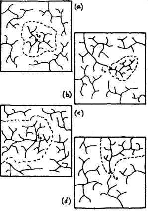
FIG. 2.: Two component spanning trees corresponding to: (a) general, (b) last, (c) dissipating and (d) dissipating last waves.

Indeed, let us consider all waves that, being initiated somewhere in the bulk of the system, propagate to the boundary and dissipate particles there. These are represented by the two-component spanning tress such that one component touches the boundary (Fig.2(c)) or the north pole of the sphere. Then, after inversion transformation this set of dissipating waves will be transformed to the set of waves that touch the south pole of the sphere. This is nothing but characteristic feature of the last wave of topplings. The probability distribution of last waves is known exactly [12]

$$W_{last}(s)~{}{\rm d}s\sim\left(\frac{a^{2}}{s}\right)^{3/8}\frac{{\rm d}s}{s}.$$ (2)

(The ultraviolet cutoff $a$ here appears because the probability is dimensionless.) Now, since the inversion transforms last waves into dissipating ones and vice versa, we conclude that after substitution $r\to R^{2}/r$ the probability distribution of last waves gets the probability distribution of dissipating waves. In this way, we obtain

$$W_{diss}(s)~{}{\rm d}s\sim\left(\frac{s}{L^{2}}\right)^{3/8}\frac{{\rm d}s}{s}.$$ (3)

Then, if we consider only those dissipating waves that are also last in an avalanche then we can notice that such waves touch both the boundary of the system and the site where avalanche was initiated. So, their distribution should be invariant under inversion transformation, $r\to R^{2}/r$. The only such a distribution is

$$W_{diss~{}\!\!\&~{}\!\!last}(s)~{}{\rm d}s\sim\left(\frac{a}{L}\right)^{3/4}\frac{{\rm d}s}{s}.$$ (4)

Eq.(4) coincides with Eq.(1) up to a prefactor $\left(a/L\right)^{3/4}$. The origin of the prefactor is the following. The conformal field theory which underlies the model of dense polymers (spanning trees) has central charge $c=-2$. Saleur and Duplantier [16] proved that the dimension of the operator $\phi_{k}(\bf{r})$ that corresponds to the insertion of the polymer star with $k$ legs into the site $\bf{r}$ of the plane is equal to $\Delta_{k}=(k^{2}-1)/4$. The polymer star is formed by $k$ different branching polymers joined at the site $\bf{r}$ and connecting the site with the boundary of the system. We can note now, that the spanning tree corresponding to a dissipating last wave form a two-leg polymer star and, hence, corresponds to the operator $\phi_{2}$ with dimension $3/4$ i.e. the average of $\phi_{2}$ should vary with the size of the system as $(a/L)^{3/4}$.

The results of our numerical simulations of these probability distributions on the lattices $L=512,1024,2048$ are shown on Fig.3. They confirm the idea of inversion symmetry with quite good accuracy. Namely, the slopes of the linear parts of the curves coincide with our theoretical predictions within the error bars $\pm 0.02$. To verify our predictions about the dependence of the probability distributions on the system size, $L$, we studied finite-size scaling with the universal scaling functions

$$W_{all}(s)~{}{\rm d}s \sim f_{1}\left(\frac{s}{L^{2}}\right)\frac{{\rm d}s}{s},$$ (6)

$$W_{diss}(s)~{}{\rm d}s \sim f_{2}\left(\frac{s}{L^{2}}\right)\frac{{\rm d}s}{s},$$ (7)

$$W_{last}(s)~{}{\rm d}s \sim L^{-3/4}f_{3}\left(\frac{s}{L^{2}}\right)\frac{{\rm d}s}{s},$$ (8)

$$W_{diss~{}\!\!\&~{}\!\!last}(s)~{}{\rm d}s \sim L^{-3/4}f_{4}\left(\frac{s}{L^{2}}\right)\frac{{\rm d}s}{s}.$$ (9)

The collapse of our data for different lattices $L=512,1024,2048$ is shown on Fig.4.

FIG. 3.: This picture shows the distribution of all (solid line), last (dashed line), boundary (dotted line) and last waves that touch the boundary (dash dotted line).

FIG. 4.: This picture shows the collapse of our data in the finite-size analysis.

Up to now we have only been concerned about one-wave probability distributions. These obey relatively simple scaling laws since they reflect rather static than dynamical properties of the sandpile model. The very first step towards understanding of quite nontrivial dynamics of the sandpile model [4, 10] is the analysis of two-wave distributions. This has recently been initiated by Paczuski and Boettcher [15] who studied numerically the transition probability distribution of the size of the next wave $P(s_{t+1}|s_{t})$, given the size of the preceding wave $s_{t}$. They suggested the following scaling form to describe their numerical data $P(s_{t+1}|s_{t})\sim s_{t+1}^{-\beta}~{}f(s_{t+1}/s_{t}),$ with the universal scaling function $f(x)$ such that $f(x\to 0)=1$ and $f(x\gg 1)\sim x^{-r}$ and scaling exponents $\beta\approx 0.75$ and $r\approx 0.5$. They, however, noticed that this scaling function pull together the curves only for the one tail of the probability distribution. The other tail remains loose. Hence, the very existence of such a universal scaling function remains dubious.

The existence of the scaling function would actually mean that wave random process is symmetric under time reversion. To clarify the issue we performed extensive numerical simulations on the lattice $L=2048$. We studied both forward, $P(s_{t+1}|s_{t})$, and backward, $P(s_{t}|s_{t+1})$, probability distributions. Our results are shown on Figs.5 and 6.

FIG. 5.: Forward conditional probability distribution $P(s_{t+1}|s_{t})$.

FIG. 6.: Backward conditional probability distribution $P(s_{t}|s_{t+1})$.

We found that asymptotics of forward probability distribution do obey scaling laws

$$P(s_{t+1}|s_{t})\sim\left\{\begin{minipage}{128.0374pt} $s_{t+1}^{-1+\gamma_{1}}$,~{}~{}{\rm if}~{}~{}$s_{t+1}\ll s_{t}$ \\ $s_{t+1}^{-1-\gamma_{2}}$,~{}~{}{\rm if}~{}~{}$s_{t+1}\gg s_{t}$ \end{minipage}\right.$$ (10)

with scaling exponent $\gamma_{1}\approx\gamma_{2}\approx 1/4$ proposed by Paczuski and Boettcher [15]. However, for backward in time probability distribution we found different asymptotics

$$P(s_{t}|s_{t+1})\sim\left\{\begin{minipage}{128.0374pt} $s_{t}^{-1+\delta_{1}}$,~{}~{}{\rm if}~{}~{}$s_{t}\ll s_{t+1}$ \\ $s_{t}^{-1-\delta_{2}}$,~{}~{}{\rm if}~{}~{}$s_{t}\gg s_{t+1}$ \end{minipage}\right.$$ (11)

with scaling exponent $\delta_{1}\approx\delta_{2}\approx 3/8$. Hence, according to our numerical simulations the wave process is not symmetrical under ”time” reversion.

The explanation of this asymmetry is still the problem for the future. Scaling arguments, however, can be given in favor of the hypothesis that the exponent 3/8 is exact. First of all, in the limit $s_{t+1}\to a^{2}$ the backward conditional probability $P(s_{t}|s_{t+1})$ should coincide with the probability distribution of the very last waves in avalanches. Indeed, in this limit every wave of topplings which is much smaller then the preceding one necessarily touches somewhere the boundary of the preceding wave. Now, if we coarse grain the picture in such a way that the size of the next wave $s_{t+1}$ becomes comparable with the unit cell of new coarse grained lattice, then the geometry of the picture will resemble that of last waves of topplings with the wave $s_{t+1}$ playing the role of the origin of the avalanche on that scale. Hence, the factor $(a^{2}/s)^{3/8}$ in Eq.(2) corresponds to the factor $(s_{t+1}/s_{t})^{3/8}$ in the distribution

$$P(s_{t}|s_{t+1})\sim\left(\frac{s_{t+1}}{s_{t}}\right)^{3/8}\frac{{\rm d}s_{t}}{s_{t}}$$ (12)

in the limit $s_{t}\gg s_{t+1}$ From this it follows that exponent $\delta_{2}=3/8$ should be exact. Also, if we assume that the inversion symmetry is valid not only for one-wave but also for two-wave distributions we get scaling relations $\gamma_{1}=\gamma_{2}$ and $\delta_{1}=\delta_{2}$.

This work was supported by the Russian Foundation for Basic Research through Grants No. 99-01-00882 and National Science Council of the Republic of China (Taiwan) under grant No. NSC 89-2112-M001-005.

REFERENCES

- [1] P. Bak, C. Tang, and K. Wiesenfeld, Phys. Rev. Lett. 59 (1987) 381.
- [2] A.N. Kolmogorov, C. R. Acad. Sci. USSR 30 (1941) 301.
- [3] M. Kardar, G. Parisi and Y.-C. Zhang, Phys. Rev. Lett. 56,889 (1986).
- [4] L.P. Kadanoff, S.R. Nagel, L. Wu and S.M. Zhou, Phys. Rev. A 39 (1989) 6524; S.S. Manna, J. Stat. Phys. 59 (1990) 509; P. Grassberger and S.S. Manna, J. Phys. France 51 (1990) 1077.
- [5] D. Dhar, Phys. Rev. Lett. 64 (1990) 1613.
- [6] S.N. Majumdar and D. Dhar, Physica A 185 (1992) 129.
- [7] S.N. Majumdar and D. Dhar, J. Phys. A 24 (1991) L357.
- [8] V.B. Priezzhev, J. Stat. Phys. 74 (1994) 955.
- [9] E.V. Ivashkevich, J. Phys. A 27 (1994) 3643.
- [10] M. De Menech, A.L. Stella and C. Tebaldi, Phys. Rev. E 58 (1998) R2677;
- [11] E.V. Ivashkevich, D.V. Ktitarev and V.B. Priezzhev, Physica A 209 (1994) 347.
- [12] D. Dhar and S.S. Manna, Phys. Rev. E 49 (1994) 2684.
- [13] E.V. Ivashkevich, D.V. Ktitarev and V.B. Priezzhev, J. Phys. A 27 (1994) L585.
- [14] V.B. Priezzhev, D.V. Ktitarev and E.V. Ivashkevich, Phys. Rev. Lett. 76 (1996) 2093.
- [15] M. Paszuski and S. Boettcher, Phys. Rev. E 56 (1997) R3745.
- [16] H. Saleur and B. Duplantier, Phys.Rev.Lett. 58 (1987) 2325.