Correlated Persistent Tunneling Currents in Glasses

Abstract

Low temperature properties of glasses are derived within a generalized tunneling model, considering the motion of charged particles on a closed path in a double-well potential. The presence of a magnetic induction field $\textstyle B$ violates the time reversal invariance due to the Aharonov-Bohm phase, and leads to flux periodic energy levels. At low temperature, this effect is shown to be strongly enhanced by dipole-dipole and elastic interactions between tunneling systems and becomes measurable. Thus, the recently observed strong sensitivity of the electric permittivity to weak magnetic fields can be explained. In addition, superimposed oscillations as function of the magnetic field are predicted. PACS- numbers: 61.43 Fs, 66.35.+a, 77.22.Ch, 03.65.Bz

At low temperature, glasses exhibit a variety of surprising properties of considerable theoretical interest. They are attributed to the existence of low-energy excitations present in nearly all amorphous solids and disordered crystals [2]. In the standard tunneling model (STM) these excitations are described on a phenomenological basis by noninteracting two-level tunneling systems (TLS’s)[3]. Such a TLS can be approximately treated as a particle moving in a double-well potential. At sufficiently low temperature only the ground states in the two wells are relevant, and the system is effectively restricted to the two-dimensional Hilbert space. Thus, the Hamiltonian of a TLS has the form $H_{0}=(1/2)(\Delta\sigma_{z}-\Delta_{0}\sigma_{x})$, where $\Delta$ and $\Delta_{0}$ are the asymmetry energy and the tunneling matrix element, respectively. Because of the random structure of glasses it is assumed that $\Delta$ and $\Delta_{0}$ exhibit a wide distribution according to $P(\Delta,\Delta_{0})=\bar{P}/\Delta_{0}$, where $\bar{P}$ is a constant. Treating the coupling of TLS’s with external acoustic and electric fields as a weak perturbation of $H_{0}$, the STM has successfully explained many of the anomalous thermal, acoustic and dielectric low-temperature properties of glasses. Deviations from the predictions of the STM [4] have been usually reduced to interaction between TLS’s [5]. Based on the spin-Boson-Hamiltonian, the elastic interaction between TLS’s can be investigated in a nonperturbative manner [6]. In that way it can be demonstrated that the strong TLS-phonon coupling essentially leads to a renormalization of the tunneling parameters, $\bar{P}$ and $\Delta_{\rm 0min}$, and thus to the quasiparticle picture of phonon-dressed TLS’s. It must be asked, however, whether interaction can also lead to an observable action of electromagnetic fields on the quantum-mechanical state of TLS’s. This is motivated by the recently reported strong sensitivity of the electric permittivity (dielectric constant) to weak magnetic fields in multicomponent glasses at ultra-low temperature [7]. The purpose of the present paper is therefore, to investigate the influence of static electromagnetic fields on the energy spectrum of a TLS, and how it is modified by the coupling between them.

In order to estimate electromagnetic field effects upon the electric permittivity of glasses in a classical approach, we can start from general thermodynamic principles, treating glasses as isotropic non-viscous dielectrics devoid of any free charges and free currents. The constitutive quantities of such a material can depend on mass density $\rho$, velocity $\textstyle\dot{x}$, temperature $T$, temperature gradient ${\bf\nabla}T$, electric field $\textstyle E$ and magnetic flux density $\textstyle B$. The general form of the constitutive equation for a constitutive quantity such as the polarization $\mathchoice{{\hbox{\boldmath$\displaystyle P$}}}{{\hbox{\boldmath$\textstyle P$}}}{{\hbox{\boldmath$\scriptstyle P$}}}{{\hbox{\boldmath$\scriptscriptstyle P$}}}=\mathchoice{{\hbox{\boldmath$\displaystyle P$}}}{{\hbox{\boldmath$\textstyle P$}}}{{\hbox{\boldmath$\scriptstyle P$}}}{{\hbox{\boldmath$\scriptscriptstyle P$}}}[\rho,\mathchoice{{\hbox{\boldmath$\displaystyle\dot{x}$}}}{{\hbox{\boldmath$\textstyle\dot{x}$}}}{{\hbox{\boldmath$\scriptstyle\dot{x}$}}}{{\hbox{\boldmath$\scriptscriptstyle\dot{x}$}}},T,\nabla T,\mathchoice{{\hbox{\boldmath$\displaystyle E$}}}{{\hbox{\boldmath$\textstyle E$}}}{{\hbox{\boldmath$\scriptstyle E$}}}{{\hbox{\boldmath$\scriptscriptstyle E$}}},\mathchoice{{\hbox{\boldmath$\displaystyle B$}}}{{\hbox{\boldmath$\textstyle B$}}}{{\hbox{\boldmath$\scriptstyle B$}}}{{\hbox{\boldmath$\scriptscriptstyle B$}}}]$ is restricted by the principle of material frame indifference (or objectivity, PMO) and the entropy principle [8]. With respect to Euclidean transformations, $\mathchoice{{\hbox{\boldmath$\displaystyle x$}}}{{\hbox{\boldmath$\textstyle x$}}}{{\hbox{\boldmath$\scriptstyle x$}}}{{\hbox{\boldmath$\scriptscriptstyle x$}}}^{*}=\mathchoice{{\hbox{\boldmath$\displaystyle O(t)$}}}{{\hbox{\boldmath$\textstyle O(t)$}}}{{\hbox{\boldmath$\scriptstyle O(t)$}}}{{\hbox{\boldmath$\scriptscriptstyle O(t)$}}}\mathchoice{{\hbox{\boldmath$\displaystyle x$}}}{{\hbox{\boldmath$\textstyle x$}}}{{\hbox{\boldmath$\scriptstyle x$}}}{{\hbox{\boldmath$\scriptscriptstyle x$}}}+\mathchoice{{\hbox{\boldmath$\displaystyle b(t)$}}}{{\hbox{\boldmath$\textstyle b(t)$}}}{{\hbox{\boldmath$\scriptstyle b(t)$}}}{{\hbox{\boldmath$\scriptscriptstyle b(t)$}}}$, where $\mathchoice{{\hbox{\boldmath$\displaystyle b$}}}{{\hbox{\boldmath$\textstyle b$}}}{{\hbox{\boldmath$\scriptstyle b$}}}{{\hbox{\boldmath$\scriptscriptstyle b$}}}(t)$ and $\mathchoice{{\hbox{\boldmath$\displaystyle O$}}}{{\hbox{\boldmath$\textstyle O$}}}{{\hbox{\boldmath$\scriptstyle O$}}}{{\hbox{\boldmath$\scriptscriptstyle O$}}}(t)$ determine the translation of two frames and the relative rotation of their axes, respectively, the PMO states that the constitutive equations must be invariant under change of frame. This means that $\textstyle\dot{x}$ and $\textstyle E$ cannot occur separately as variables, but only in combination as electromotive intensity $\mathchoice{{\hbox{\boldmath$\displaystyle\cal E$}}}{{\hbox{\boldmath$\textstyle\cal E$}}}{{\hbox{\boldmath$\scriptstyle\cal E$}}}{{\hbox{\boldmath$\scriptscriptstyle\cal E$}}}=\mathchoice{{\hbox{\boldmath$\displaystyle E$}}}{{\hbox{\boldmath$\textstyle E$}}}{{\hbox{\boldmath$\scriptstyle E$}}}{{\hbox{\boldmath$\scriptscriptstyle E$}}}+\mathchoice{{\hbox{\boldmath$\displaystyle\dot{x}$}}}{{\hbox{\boldmath$\textstyle\dot{x}$}}}{{\hbox{\boldmath$\scriptstyle\dot{x}$}}}{{\hbox{\boldmath$\scriptscriptstyle\dot{x}$}}}\times\mathchoice{{\hbox{\boldmath$\displaystyle B$}}}{{\hbox{\boldmath$\textstyle B$}}}{{\hbox{\boldmath$\scriptstyle B$}}}{{\hbox{\boldmath$\scriptscriptstyle B$}}}$. For the polarization the functional equation $\mathchoice{{\hbox{\boldmath$\displaystyle P$}}}{{\hbox{\boldmath$\textstyle P$}}}{{\hbox{\boldmath$\scriptstyle P$}}}{{\hbox{\boldmath$\scriptscriptstyle P$}}}[\rho,T,\mathchoice{{\hbox{\boldmath$\displaystyle O$}}}{{\hbox{\boldmath$\textstyle O$}}}{{\hbox{\boldmath$\scriptstyle O$}}}{{\hbox{\boldmath$\scriptscriptstyle O$}}}\nabla T,\mathchoice{{\hbox{\boldmath$\displaystyle O$}}}{{\hbox{\boldmath$\textstyle O$}}}{{\hbox{\boldmath$\scriptstyle O$}}}{{\hbox{\boldmath$\scriptscriptstyle O$}}}\mathchoice{{\hbox{\boldmath$\displaystyle\cal E$}}}{{\hbox{\boldmath$\textstyle\cal E$}}}{{\hbox{\boldmath$\scriptstyle\cal E$}}}{{\hbox{\boldmath$\scriptscriptstyle\cal E$}}},(\rm{det}\mathchoice{{\hbox{\boldmath$\displaystyle O$}}}{{\hbox{\boldmath$\textstyle O$}}}{{\hbox{\boldmath$\scriptstyle O$}}}{{\hbox{\boldmath$\scriptscriptstyle O$}}})\mathchoice{{\hbox{\boldmath$\displaystyle O$}}}{{\hbox{\boldmath$\textstyle O$}}}{{\hbox{\boldmath$\scriptstyle O$}}}{{\hbox{\boldmath$\scriptscriptstyle O$}}}\mathchoice{{\hbox{\boldmath$\displaystyle B$}}}{{\hbox{\boldmath$\textstyle B$}}}{{\hbox{\boldmath$\scriptstyle B$}}}{{\hbox{\boldmath$\scriptscriptstyle B$}}}]=\mathchoice{{\hbox{\boldmath$\displaystyle O$}}}{{\hbox{\boldmath$\textstyle O$}}}{{\hbox{\boldmath$\scriptstyle O$}}}{{\hbox{\boldmath$\scriptscriptstyle O$}}}\mathchoice{{\hbox{\boldmath$\displaystyle P$}}}{{\hbox{\boldmath$\textstyle P$}}}{{\hbox{\boldmath$\scriptstyle P$}}}{{\hbox{\boldmath$\scriptscriptstyle P$}}}[\rho,T,\nabla T,\mathchoice{{\hbox{\boldmath$\displaystyle\cal E$}}}{{\hbox{\boldmath$\textstyle\cal E$}}}{{\hbox{\boldmath$\scriptstyle\cal E$}}}{{\hbox{\boldmath$\scriptscriptstyle\cal E$}}},\mathchoice{{\hbox{\boldmath$\displaystyle B$}}}{{\hbox{\boldmath$\textstyle B$}}}{{\hbox{\boldmath$\scriptstyle B$}}}{{\hbox{\boldmath$\scriptscriptstyle B$}}}]$ must be satisfied for all orthogonal matrices $\textstyle O$. Recall that $\textstyle P$ and $\textstyle\cal E$ are polar vectors, while $\textstyle B$ is an axial vector. The general solution of the functional equation leads to the representation for the polarization, whose equilibrium part ($\nabla T=0$) is given by $\mathchoice{{\hbox{\boldmath$\displaystyle P$}}}{{\hbox{\boldmath$\textstyle P$}}}{{\hbox{\boldmath$\scriptstyle P$}}}{{\hbox{\boldmath$\scriptscriptstyle P$}}}/\epsilon_{0}=\chi_{1}\mathchoice{{\hbox{\boldmath$\displaystyle\cal E$}}}{{\hbox{\boldmath$\textstyle\cal E$}}}{{\hbox{\boldmath$\scriptstyle\cal E$}}}{{\hbox{\boldmath$\scriptscriptstyle\cal E$}}}+\chi_{2}(\mathchoice{{\hbox{\boldmath$\displaystyle B$}}}{{\hbox{\boldmath$\textstyle B$}}}{{\hbox{\boldmath$\scriptstyle B$}}}{{\hbox{\boldmath$\scriptscriptstyle B$}}}\cdot\mathchoice{{\hbox{\boldmath$\displaystyle\cal E$}}}{{\hbox{\boldmath$\textstyle\cal E$}}}{{\hbox{\boldmath$\scriptstyle\cal E$}}}{{\hbox{\boldmath$\scriptscriptstyle\cal E$}}})\mathchoice{{\hbox{\boldmath$\displaystyle B$}}}{{\hbox{\boldmath$\textstyle B$}}}{{\hbox{\boldmath$\scriptstyle B$}}}{{\hbox{\boldmath$\scriptscriptstyle B$}}}+\chi_{3}\mathchoice{{\hbox{\boldmath$\displaystyle B$}}}{{\hbox{\boldmath$\textstyle B$}}}{{\hbox{\boldmath$\scriptstyle B$}}}{{\hbox{\boldmath$\scriptscriptstyle B$}}}\times\mathchoice{{\hbox{\boldmath$\displaystyle\cal E$}}}{{\hbox{\boldmath$\textstyle\cal E$}}}{{\hbox{\boldmath$\scriptstyle\cal E$}}}{{\hbox{\boldmath$\scriptscriptstyle\cal E$}}}$. The susceptibilities $\chi_{\alpha}$ can still depend on the scalars $\rho,T,{\cal E}^{2},B^{2}$ and $(\mathchoice{{\hbox{\boldmath$\displaystyle\cal E$}}}{{\hbox{\boldmath$\textstyle\cal E$}}}{{\hbox{\boldmath$\scriptstyle\cal E$}}}{{\hbox{\boldmath$\scriptscriptstyle\cal E$}}}\cdot\mathchoice{{\hbox{\boldmath$\displaystyle B$}}}{{\hbox{\boldmath$\textstyle B$}}}{{\hbox{\boldmath$\scriptstyle B$}}}{{\hbox{\boldmath$\scriptscriptstyle B$}}})^{2}$. As a further restriction, it follows from the entropy principle that $\chi_{3}=0.$ Consequently, the electric permittivity $\epsilon=1+\chi_{1}+\chi_{2}B_{z}^{2}$ of a rigid ($\mathchoice{{\hbox{\boldmath$\displaystyle\dot{x}$}}}{{\hbox{\boldmath$\textstyle\dot{x}$}}}{{\hbox{\boldmath$\scriptstyle\dot{x}$}}}{{\hbox{\boldmath$\scriptscriptstyle\dot{x}$}}}=0$) dielectric and magnetizable glass, determined by capacitance measurement in a plate condenser with $\mathchoice{{\hbox{\boldmath$\displaystyle E$}}}{{\hbox{\boldmath$\textstyle E$}}}{{\hbox{\boldmath$\scriptstyle E$}}}{{\hbox{\boldmath$\scriptscriptstyle E$}}}=(0,0,E_{z})$, is expected to depend on $E_{z}^{2}$ and $B^{2}$ (and besides on $B^{4}$, if $\mathchoice{{\hbox{\boldmath$\displaystyle B$}}}{{\hbox{\boldmath$\textstyle B$}}}{{\hbox{\boldmath$\scriptstyle B$}}}{{\hbox{\boldmath$\scriptscriptstyle B$}}}||\mathchoice{{\hbox{\boldmath$\displaystyle E$}}}{{\hbox{\boldmath$\textstyle E$}}}{{\hbox{\boldmath$\scriptstyle E$}}}{{\hbox{\boldmath$\scriptscriptstyle E$}}}$). The quadratic field dependence of $\epsilon$ was indeed reported to be valid for some glasses [9]. In general, however, glasses are properly assumed to be linear dielectrics, so that $\epsilon(\rho,T)$ does not depend on the electromagnetic field. Several glasses do not show any measurable changes of their electric permittivity up to high magnetic fields and temperatures down to a few mK [10]. The recently observed magnetic field dependence of $\epsilon$ in multicomponent glasses at ultra-low temperature [7], however, is completely different in nature from the magnetoeffect in nonlinear dielectrics, and cannot be derived from thermodynamics assuming glasses as simple magnetizable dielectrics. The knowledge of the local field strengths $\textstyle B$ and $\textstyle E$ only is not sufficient for the consistent description of electromagnetic field effects on the quantum-mechanical state of charged particles [11]. For that reason the influence of a magnetic field on the energy spectrum of a TLS should be investigated from a microscopic point of view. In order to describe a TLS in a magnetic field the three-dimensional motion of a charged particle in an electrostatic double-well potential has to be considered. Imagine a hat like potential with two potential barriers in azimuthal direction along the rim of the hat as shown in Fig. 1.

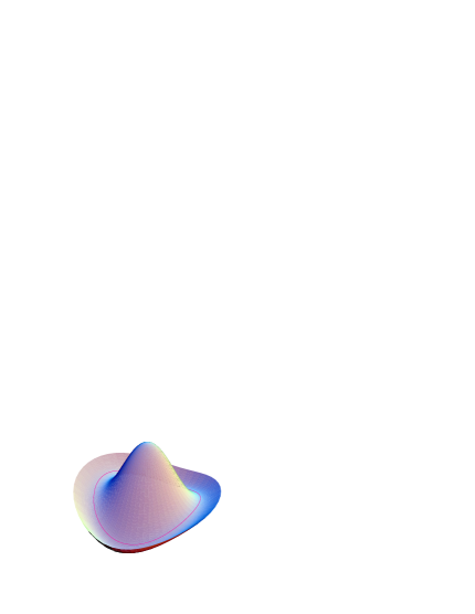
FIG. 1.: Hat potential. The double-well potential for a charged particle confined to a circular path is indicated by the line. The induction field $\textstyle B$ can have an arbitrary angle with the plane of motion

The Hamiltonian for a non-relativistic and spinless charged particle of mass $m$ and charge $q$, which moves in an uniform induction field $\textstyle B$ and in an electrostatic potential $V$, is given by

$$H_{0}=(\mathchoice{{\hbox{\boldmath$\displaystyle p$}}}{{\hbox{\boldmath$\textstyle p$}}}{{\hbox{\boldmath$\scriptstyle p$}}}{{\hbox{\boldmath$\scriptscriptstyle p$}}}-Q\mathchoice{{\hbox{\boldmath$\displaystyle A$}}}{{\hbox{\boldmath$\textstyle A$}}}{{\hbox{\boldmath$\scriptstyle A$}}}{{\hbox{\boldmath$\scriptscriptstyle A$}}})^{2}/(2m)+V.$$ (1)

The symmetric gauge for the vector potential $\mathchoice{{\hbox{\boldmath$\displaystyle A$}}}{{\hbox{\boldmath$\textstyle A$}}}{{\hbox{\boldmath$\scriptstyle A$}}}{{\hbox{\boldmath$\scriptscriptstyle A$}}}=(0,Br/2,0)$ is appropriate to cylindrical co-ordinates $(r,\theta,z)$. An uniform induction field $B$ along the $z$ axis forces the charged particle to circular motion in the perpendicular plane at radii $r_{n}$ with $B\pi r_{n}^{2}=\phi_{0}n$, where $\phi_{0}=h/Q$ is the flux quantum, and $n$ an arbitrary integer. The magnetic length $l_{B}=\sqrt{\hbar/(QB)}$ characterizes the strength of this magnetic confinement and has to be compared with the radius $r_{V}$ at which the particle is restrained by an electrostatic potential $V(r,\theta,z)$ of the form shown in Fig. 1. For weak magnetic fields, $r_{V}\ll l_{B}$, the confinement force due to $V$ exceeds the Lorentz force, and Landau quantization does not appear. In that case, the problem is reduced to that of an one-dimensional ring of radius $r$, with the Hamiltonian

$$H_{0}=\frac{1}{2m}(-i\hbar\frac{1}{r}\frac{\partial}{\partial\theta}-Q{A_{\theta}})^{2}+V(\theta),$$ (2)

where $A_{\theta}=Br/2=\phi/(2\pi r)$. In the more general case that the induction field $B$ has an arbitrary angle $\alpha$ with the plane of motion, the magnetic flux through the circular orbit of a TLS is given by $\phi=B\pi r^{2}$cos$\alpha$.

For a double-well potential $V(\theta)=V\cos(2\theta)$, the Schrödinger equation can be reduced by means of the gauge transformation $\tilde{\varphi}(\theta)=\exp(-i\theta\phi/\phi_{0})\varphi(\theta)$ to the Mathieu equation $\partial^{2}\tilde{\varphi}/\partial\theta^{2}+(E/a-(V/a)\cos(2\theta))\hat{\varphi}=0$, where the energy $E$ and the potential amplitude $V$ enter in units of $a=\hbar^{2}/(2mr^{2})$. Thereby, the magnetic flux is removed from the Hamiltonian, and the periodic boundary conditions $\varphi(\theta+2\pi)=\varphi(\theta)$ are substituted by the magnetic flux twisted boundary conditions $\tilde{\varphi}(\theta+2\pi)=\exp(-i2\pi\phi/\phi_{0})\tilde{\varphi}(\theta)$. Solutions with these boundary conditions do exist for particular values of the ratio $E/a$, which yield the energy eigenvalues. They are periodic in the magnetic flux $\phi/\phi_{0}$ as seen in Fig. 2, where the energies $E_{-}$ and $E_{+}$ of the ground and the first excited state are plotted.

FIG. 2.: The two lowest energy eigenvalues as function of the flux ratio $\phi/\phi_{0}$ through the circular path of a charged particle in a symmetric double-well potential

For non-zero magnetic flux $\phi$ the energy eigenfunctions composed of the odd and even Mathieu functions become complex. Thus, due to the magnetic induction field both the parity and the time reversal invariance of the TLS are broken. Each energy eigenstate does carry a persistent current [12] of opposite direction, given by

$$I_{\pm}(\varphi)=\partial E_{\pm}(\phi)/\partial\phi.$$ (3)

A net persistent tunneling current results in a magnetic moment of the TLS.

For more general double-well potentials, allowing also an asymmetry $\Delta$ in the energy of the two minima, the harmonic approximation of the potential can be done around each minimum, in analogy to the STM. Then, the ground state and the first excited state of the TLS can be well approximated by a superposition of the ground states of each harmonic oscillator, if $V\gg\hbar\Omega>\Delta$, where $\Omega$ is the oscillator frequency and $V\approx(1/8)m\Omega^{2}\pi^{2}r^{2}$ is the potential barrier. The energy eigenvalues are found to be $E_{\pm}=(\hbar\Omega+\Delta\pm E_{\rm g}(\phi))/2$, giving the excitation energy (gap),

$$E_{\rm g}(\phi)=\sqrt{\Delta^{2}+t(\phi)^{2}},$$ (4)

where $t(\phi)=\Delta_{0}\cos(\pi\phi/\phi_{0}),$ with $\Delta_{0}\approx\hbar\Omega\exp(-\lambda)$ and $\lambda=2V/(\hbar\Omega)>1$. This is identical to the STM, when there the tunneling parameter $\Delta_{0}$ is substituted by the magnetic flux dependent tunneling splitting $t(\phi)$.

The low-temperature thermodynamic properties calculated in the generalized model of independent TLS’s, which are determined by the energy spectrum $E_{\rm g}(\phi)$, are consequently periodic functions of the magnetic flux with a period of $\phi_{0}$. Thus, the TLS energy density $e(\phi,T)$ can be obtained by averaging the excitation energy over the parameters $\Delta$ and $\Delta_{0}$, according to

$$e(\phi,T)=\bar{P}\int\frac{\mbox{d}\Delta_{0}}{\Delta_{0}}\int\mbox{d}\Delta\frac{E_{g}}{\exp[E_{g}/(k_{B}T)]+1}.$$ (5)

For temperatures $T\gg\Delta_{\rm 0min}/k_{\rm B}$ the specific heat, $c(\phi,T)=1/\rho\cdot\partial e(\phi,T)/\partial T$, is approximately given by

$$c(\phi,T)=\frac{\pi^{2}}{6\rho}\cdot\bar{P}k_{\rm B}^{2}T\Bigl{[}1+\ln\Bigl{(}\frac{2k_{\rm B}T}{\mid t_{\rm min}(\phi)\mid}\Bigr{)}\Bigr{]},$$ (6)

where $t_{\rm min}(\phi)=\Delta_{\rm 0min}\cdot\cos(\pi\phi/\phi_{0})$ is the flux dependent minimal tunneling splitting. The presence of an external electrical field $\textstyle E$ produces an interaction energy of a TLS with the dipole moment $\textstyle p$ of amount $H_{\rm int}=-\mathchoice{{\hbox{\boldmath$\displaystyle p$}}}{{\hbox{\boldmath$\textstyle p$}}}{{\hbox{\boldmath$\scriptstyle p$}}}{{\hbox{\boldmath$\scriptscriptstyle p$}}}\cdot\mathchoice{{\hbox{\boldmath$\displaystyle E$}}}{{\hbox{\boldmath$\textstyle E$}}}{{\hbox{\boldmath$\scriptstyle E$}}}{{\hbox{\boldmath$\scriptscriptstyle E$}}}$. Due to $\textstyle E$ the asymmetry of the TLS is changed, while the change in the tunneling splitting can be neglected for $\bf p\cdot\bf E\ll V$. The thermodynamic polarization, $\mathchoice{{\hbox{\boldmath$\displaystyle P$}}}{{\hbox{\boldmath$\textstyle P$}}}{{\hbox{\boldmath$\scriptstyle P$}}}{{\hbox{\boldmath$\scriptscriptstyle P$}}}=-\langle\partial\hat{H}/\partial\mathchoice{{\hbox{\boldmath$\displaystyle E$}}}{{\hbox{\boldmath$\textstyle E$}}}{{\hbox{\boldmath$\scriptstyle E$}}}{{\hbox{\boldmath$\scriptscriptstyle E$}}}\rangle$, can be derived from the effective Hamiltonian $\hat{H}=H_{0}+H_{\rm int}$. The ensemble average over the different TLS’s is done by averaging over possible dipole orientations and the parameters $\Delta$ and $\Delta_{0}$ with the measure $\bar{P}\cdot d\Delta d\Delta_{0}/\Delta_{0}$. As a result, the resonant part of the electric permittivity $\epsilon_{\rm res}$ becomes in linear response ($\mathchoice{{\hbox{\boldmath$\displaystyle P$}}}{{\hbox{\boldmath$\textstyle P$}}}{{\hbox{\boldmath$\scriptstyle P$}}}{{\hbox{\boldmath$\scriptscriptstyle P$}}}=\epsilon_{0}(\epsilon-1)\mathchoice{{\hbox{\boldmath$\displaystyle E$}}}{{\hbox{\boldmath$\textstyle E$}}}{{\hbox{\boldmath$\scriptstyle E$}}}{{\hbox{\boldmath$\scriptscriptstyle E$}}}$),

$$\epsilon_{\rm res}-1=\frac{2\bar{P}p^{2}}{3\epsilon_{0}}\int_{\mid t_{\rm min}(\phi)\mid}^{E_{\rm max}}\mbox{d}E_{\rm g}\frac{\sqrt{E_{\rm g}^{2}-t_{\rm min}(\phi)^{2}}}{E_{\rm g}^{2}}\tanh(\frac{E_{\rm g}}{2k_{\rm B}T}).$$ (7)

The electric permittivity depends on temperature as well as magnetic flux through the minimal tunneling splitting. There are maxima in $\epsilon_{\rm res}(\phi,T)$ at $\phi/\phi_{0}=(2n+1)/2$, $n=0,1,2,...,$ where the lower cutoff of the excitation energy vanishes. These maxima become more pronounced as the temperature is lowered. Thus, the resonant part $\epsilon_{\rm res}$ does depend on the magnetic field at low temperature where the relaxational contribution to the permittivity $\epsilon_{\rm rel}$ is negligible. Indeed, the theoretically derived dependence of the electric permittivity, Eq. (7), on magnetic field and temperature explains qualitatively the main feature of the experimental results obtained in multicomponent glasses [13] as shown in Fig. 3.

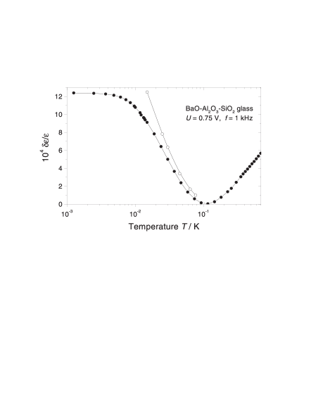
FIG. 3.: Temperature variation of the electric permittivity $\delta\epsilon/\epsilon=[\epsilon(T)-\epsilon(T_{\rm 0})]/\epsilon(T_{\rm 0})$ of a BaO-Al ₂O₃-SiO₂ glass measured at a frequency of 1 kHz and a voltage of 0.75 V (data from Ref. (12)). $T_{\rm 0}$=113 mK was taken as a reference. The solid circles represent the data in zero field, whereas the open circles represent the maximal measured increase of $\epsilon$ due to a magnetic field. As shown by the solid lines, the data can be described by Eq.(7) in the resonant regime below 100 mK with $t_{\rm min}(\phi=0)/{\rm k_{B}}=12.2$ mK (lower line) and $t_{\rm min}(\phi=\phi_{0}/2)=0$ (upper line), respectively. Above 100 mK the relaxational part $\epsilon_{\rm rel}$ in $\epsilon$ is additionally taken into account.

In the low-temperature resonant regime, the measured temperature dependence of $\epsilon(T,\phi=0)$ can be well described by Eq.(7) assuming $\bar{P}p^{2}/\epsilon_{0}=1.03\cdot 10^{-2}$ and $\Delta_{\rm 0min}/k_{\rm B}=12.2$ mK. The deviation from the logarithmic temperature dependence of $\epsilon_{\rm res}$ (dielectric saturation [14]) is lifted at magnetic fields where $\epsilon_{\rm res}(T,\phi=\phi_{0}/2)$ becomes maximal. In that case, the lower cutoff $t_{\rm min}(\phi)$ vanishes, and $\epsilon$ varies logarithmically with temperature. The remarkable result of the experiments consists in the fact that both the calculated logarithmic temperature dependence of $\epsilon_{\rm res}$ and its slope relative to the relaxational part $\epsilon_{\rm rel}$ of (-2):1 at higher temperature is achieved even at weak magnetic fields of about 0.1 T. The experimentally observed maximum in $\epsilon(T,\phi(B))$ at $B\approx 0.1$ T, which slightly depends on temperature, requires to assume for $r\approx 2\cdot 10^{-10}$ m the TLS charge of $Q\approx 4\cdot 10^{5}|\rm{e}|$, where e is the elementary charge. Before we discuss the origin of such a large value of $Q$ resulting apparently from interactions of TLS’s, we want to mention that the experiments described in [13], which were stimulated by our theoretical findings, have confirmed a corresponding flux periodic behaviour of both the specific heat and the electric permittivity. It should be noted that $\phi$ in Eqs. (6) and (7) has to be interpreted as an effective magnetic flux, and an averaging over orientations and charges of TLS’s must be carried out in order to analyze precisely the oscillatory behaviour of $c(T,\phi)$ and $\epsilon(T,\phi)$ in magnetic fields.

In order to explain the large values of $Q$, we have to consider the excitation spectrum of coupled rings. The Hamiltonian is given by

$$H = \sum_{i}H_{0i}+\sum_{i\neq j}g(\theta_{i},\theta_{j})/r_{ij}^{3},$$ (8)

The first term is the sum of the Hamiltonians of the uncoupled rings, Eq. (2). The second term is the (dipole-dipole or elastic) interaction energy decaying with the distance $r_{ij}$ between two TLS’s $i$, $j$, and depends on the orientations of the dipole moments as parametrized by the angles $\theta_{i}$. We find [15] when the interaction energy exceeds the typical kinetic energy scale in each ring, that the excitation spectrum of strongly coupled rings equals that of one ring with an effective charge $Q$, which is the sum of the charges of the rings. This is intuitively clear, since then the motion of the tunneling particles is governed by the interaction between them, making all degrees of freedom massive apart from their center of mass motion. Thus, we have identified a possible origin for large values of Q. Similar situations, where the tiny magetic response of microscopic entities like a molecule is enhanced to a macroscopic magnetic field effect due to correlations between them, are known. One example is the Frederiks transition in nematic liquid crystals[16]. Assuming for the tunneling parameters the feasible values $\bar{P}=10^{45}\rm{J}^{-1}\rm{m}^{-3}$, $E_{\rm{max}}/\rm k_{B}=5$ K, $\Delta_{\rm{0min}}/\rm{k_{B}}=10^{-6}$ K, the average distance between TLS’s can be estimated to be $r_{nn}=10^{-8}$ m. Thus, a number $10^{5}$ of coupled rings implies mesoscopic coherence lengths, on the order of $\mu$m. For an averaged dipole moment $p=2|e|\cdot 10^{-10}$ m, the dipole-dipole interaction energy is then $g/{\rm{k_{B}}}/r_{nn}^{3}\approx 100$ mK. This is exactly the temperature range in which the magnetic flux effects become observable. The obtained energy spectra for strongly coupled rings suggest the introduction of quasiparticles whose orbits are pierced by a flux with flux periodicity $\phi_{0}=h/Q$. They are excitations of strongly coupled TLS’s with renormalized tunneling parameters. Due to interactions the lowest quasiparticle excitation energy can be considerably changed. For example, for two coupled rings with $U>t(\phi)$ the splitting is reduced to $t(\phi)^{2}/U$.

However, there exists another phenomenon which contributes to changes in the energy spectrum and deserves special attention. It can be visualized by investigating in detail the energy levels of two interacting TLS’s[15]. The dipole moment of an asymmetrical TLS increases with decreasing tunneling splitting $t(\phi)$, and changes with variation of the external induction field. This implies that the dipolar coupling between two TLS’s depends also on $B$, and may lead to level crossings. Energy levels of the coupled system may cross when their asymmetry is unfavourable to the interaction, and when the coupling increases sufficiently with magnetic field. This is the case if, e.g., one TLS has a small tunneling splitting and hence a large dipole moment. Imagine two dipole moments, oriented such that the dipolar interaction would flip one of them. When only at higher fields the interaction is strong enough to achieve this, the first excited state and the ground state will cross in energy as function of $B$. Thus, a flip of a large total dipole moment of a coupled ring system is possible. Both level crossing and strong coupling result in quantum interference effects on a mesoscopic scale in glasses. At ultra-low temperature one may even expect a phase transition of coupled TLS’s to occur as suggested in [7]. We also expect an observable action of the electric flux on the low-temperature dielectric response of glasses in alternating electrical fields [14]. In conclusion, we derived magnetic flux effects in glasses by considering low-energy excitations as charged particles moving on closed paths in a double-well potential. Flux periodic energy levels of these tunneling states result in persistent tunneling currents. Due to strong coupling and level crossing magnetic flux effects are strongly enhanced below 100 mK and become measurable.

REFERENCES

• [1] present address.
• [2] W.A. Phillips, Rep. Prog. Phys. 50, 1657 (1987).
• [3] P.W. Anderson, B.I. Halperin, and C.M. Varma, Philos. Mag. 25, 1 (1972); W.A. Phillips, J. Low Temp. Phys. 7, 351 (1972).
• [4] P. Esquinazi ( editor ) Tunneling systems in amorphous and crystalline solids, Springer, Berlin (1998); D. Salvino, S. Rogge, B. Tigner, D. Osheroff, Phys.Rev.Lett. 73, 286 (1994).
• [5] C. C. Yu, A. J. Leggett, Commun. Condens. Mat. Phys. 14, 231 (1988), H. M. Carruzzo, E. R. Grannan, C. C. Yu, Phys. Rev. B 50, 6685 ( 1994).
• [6] K. Kassner, R. Silbey, J.Phys.: Cond. Mat. 1, 4599 (1989).
• [7] P. Strehlow, C. Enss, S. Hunklinger, Phys. Rev. Lett. 80, 5361( 1998 ).
• [8] I. MΓΌller, Thermodynamics, Pitman Advanced Publishing Program, Boston (1985).
• [9] M.J. Naughton, S. Dickinson, R.C. Samaratunga, J.S. Brooks, K.P. Martin, Rev. Sci. Instr. 54,1529 (1983).
• [10] P.J. Reijntjes, W. van Rijswijk, G.A. Vermeulen, G. Frossati, Rev.Sci.Instrum. 57, 141(1986).
• [11] L.P. Gorkov, G.M. Eliashberg, Sov. Phys. JETP 21,940 (1965).
• [12] F. Hund, Ann. Phys. (Leipzig) 32,102 (1938).
• [13] S. Hunklinger, C. Enss, P. Strehlow, Physica B 263-264, 248 (1999); P. Strehlow, M. Wohlfahrt, A. Jansen, R. Haueisen, G. Weiss, C. Enss, S. Hunklinger, to be publ..
• [14] S. Rogge, D. Natelson, B. Tigner, D. Osheroff, Phys. Rev. B 55, 11256(1997).
• [15] S. Kettemann, P. Fulde, P. Strehlow, to be published.
• [16] P. G. de Gennes and J. Prost, The Physics of Liquid Crystals, Oxford Sc. Publ., Oxford( 1993 ).