Matrix Product Approach to Conjugated Polymers

Abstract

The Matrix Product method (MPM) has been used in the past to generate variational ansatzs of the ground state (GS) of spin chains and ladders. In this paper we apply the MPM to study the GS of conjugated polymers in the valence bond basis, exploiting the charge and spin conservation as well as the electron-hole and spin-parity symmetries. We employ the $U-V-\delta$ Hamiltonian which is a simplified version of the PPP Hamiltonian. For several coupling constants $U$ and $V$ and dimerizations $\delta$ we compute the GS energy per monomer which agrees within a $2\%-4\%$ accuracy with the DMRG results. We also show the evolution of the MP-variational parameters in the weak and strong dimerization regimes.

I Introduction

The study of conjugated polymers has been a subject of great interest for over two decades. There are both theoretical and technological reasons for this interest [1]. On the theoretical side, there exists a controversy within the scientific community over how to explain, understand and describe the photophysics/photochemistry of this class of materials. This controversy is of such a fundamental nature that the solution of the problem might be in a unification of the semiconductor and metal physics with the molecular quantum chemistry. On the technological side, pi-conjugated polymers behave as semiconductors and this has prompted several research groups to investigate the physics of these materials in an effort to determine their potential for improving the performance and efficiency and reducing the cost of light-emitting diodes (LEDs). More recently, they are also considered to make an entrance in the field of photovoltaics, where they could be used as solar cells.

Saturated polymers are long chains of molecules, generally made of carbon with hydrogen on the sides, all attached to one another by single bonds. This constitutes the backbone of the macromolecule. The most relevant feature of these structures is the fact that the bonds are all single bonds or, in other words, that all the binding are of $\sigma$– type. Saturated polymers are then all very insulating; they are not electronically interesting but are known for their flexibility although they are also quite mechanically strong materials. The most familiar of these compounds is the polyethylene.

On the contrary, conjugated polymers show very interesting electronic properties together with remarkable mechanical properties; for instance, they can emit light and conduct electricity [1]. In these compounds, two of the three $2p$ orbitals on each carbon atom hybridize with the $2s$ orbital to form three $sp^{2}$ molecular orbitals. These orbitals are responsible for the backbone of the molecular chain; these are the so-called $\sigma$–orbitals. The third carbon orbital is $p_{z}$ and points perpendicular to the chain. There exist a strong overlapping between nearest-neighbours $p_{z}$ orbitals so that the corresponding electrons are fully delocalized on the whole molecule; these are the $\pi$ electrons responsible for all the interesting electronic properties of low-energy. For instance, because of these electrons, the linear chain, the polyacetylene, which is considered in this work, is dimerized: its backbone shows an alternance between double and single bonds. Quite generally , despite a huge amount of works, the electronic properties of these compound stay rather controversial [1].

The delocalization character of the electrons in the $\pi$ molecular orbitals of the conjugate polymer chains led to the introduction of model Hamiltonians to study and predict their electronic properties. The initially simplest possible model is a tight-binding approximation or Hückel model [2] to describe the motion of $\pi$ electrons in a free way. This is a very crude approximation which has been improved in several fashions. One of them is the inclusion of electron-phonon interactions [3, 4]. However, this is not enough as the electronic properties of $\pi$-conjugated polymers derive from a true many-body problem were electron-electron interactions are equally important as the electron-phonon interactions. Then, the PPP (Pariser-Parr-Pople) Hamiltonian [5, 6, 1] is used to model these electron-electron effects in a first approximation without taking into account phonon effects, to make simpler a first analysis of the electronic properties. In the PPP Hamiltonian, the alternating single-double bonds of the backbone polymer structure is realized by means of a dimerization term in the hopping kinetic energy. The most general form of the PPP Hamiltonian reads as follows:

$$H_{PPP} = H_{\rm K}+H_{\rm I},$$ (1)

$$H_{\rm K} = -\sum_{\langle i,j\rangle,\sigma}t(1-\delta(-1)^{i})(c_{i,\sigma}^{\dagger}c_{j,\sigma}+{\rm h.c.})$$ (2)

$$H_{\rm I} = U\sum_{i}(c_{i,\uparrow}^{\dagger}c_{i,\uparrow}-\frac{n_{\rm el}}{2})(c_{i,\downarrow}^{\dagger}c_{i,\downarrow}-\frac{n_{\rm el}}{2})$$ (3)

$$+ \sum_{i,j}V(r_{i,j})(\sum_{\sigma}c_{i,\sigma}^{\dagger}c_{i,\sigma}-n_{\rm el})(\sum_{\tau}c_{j,\tau}^{\dagger}c_{j,\tau}-n_{\rm el})$$ (4)

where $H_{K}$ is the dimerized tight binding kinetic part and $H_{I}$ represents the Coulomb interactions among the electrons. Here the operators $c_{i,\sigma}$, $c_{i,\sigma}^{\dagger}$ are standard creation and annihilation operators for $\pi$ electrons at carbon site $i$ with spin $\sigma$. The parameter $t$ is the hopping overlapping integral between the nearest- neighbour carbon atoms, $\delta$ measures the dimerization of the chain, $n_{\rm el}$, is the average number of electrons per site, $U$ is the on-site Coulomb repulsion between the electrons, $r_{i,j}$ is the distance between sites $i$ and $j$ along the chain and $V(r_{i,j})$ is the long range contribution of the Coulomb repulsion.

The PPP Hamiltonian has been the subject of extensive studies using a great variety of techniques such as Hartree-Fock, CI calculations, small cluster exact diagonalization, Quantum Monte Carlo and so on and so forth [1]. Only recently it has become possible to apply a new numerical technique, the Density Matrix Renormalization Group (DMRG) [7], which allows us to obtain highly accurate results both for small, intermediate and large polymer chains [8, 9, 10, 11, 12]. These DMRG studies have helped to clarify the correct ordering of excited states in the low energy part of the spectrum which are relevant for the nonlinear spectroscopic experiments.

In this paper we will concentrate on the study of the PPP Hamiltonian and leave the effect of interaction with phonons for future studies. The PPP Hamiltonian has been studied using an excitonic method based on a local description of the polymer in terms of monomers [13]. The relevant electronic configurations are built on a small number of pertinent local excitations. This has provided a simple and microscopic physical approximate picture of the model. Recently we have extended this local configuration studies using the Recurrent Variational Approach (RVA) method [14] in order to study larger polymer chains in a systematic way while retaining the previous intuitive physical picture. The RVA [15] is a non-perturbative variational method in which one retains a single state as the best candidate for the ground state of the system. This reduction of degrees of freedom is initially done in order to keep the method manageable analytically. The aim of this analytical approach is to try to understand the relevant physical degrees of freedom so that we can figure out what the underlying physics is in a strongly correlated system. This initial analytical goal has been also developed in order to later acquire more numerical precision. To do this, the method becomes more numerical and somehow stands in between an analytical formulation of the DMRG and a numerical one.

This effort of understanding the relevant electronic configurations in conjugated polymers has been also carried out in exact small cluster calculations using excitonic Valence Bond basis [16] for polymer chains of length up to 10 sites, arranged into diatomic ethylene molecules.

A first comparison of RVA results with DMRG gave us promising perspectives to improve these variational calculations [14] by incorporating more local configurations and variational parameters. In this paper we undertake this project by using a Matrix Product ansatz for the ground state (GS) wave functions [17]. This ansatz is a variational approach based on first order Recursion Relations (RR’s) instead of second order RR’s as in the RVA [18]. With this RR’s we construct the GS of the polymer chain in different symmetry sectors based on the 16 local configurations of the diatomic ethylene molecule within the PPP approximation. Thus, the chain is built up by adding one ethylene at each step of the variational process.

This paper is organized as follows. In Section 2 we introduce a Matrix Product ansatz specially adapted for the PPP Hamiltonian. In Section 3 we set up the Recurrent Relations to compute the GS energies in several sectors according to prescribed symmetries. In Section 4 we present variational and DMRG results and make a comparison obtaining a very good agreement between them. Section 5 is devoted to prospects and conclusions.

II The Matrix Product Ansatz

The main idea of the MP method is to generate the ground state (GS) of a quasi-one dimensional system in terms of a set of states $|\alpha\rangle_{N}$ generated by the following recursion formula [17, 18],

$$|\alpha\rangle_{N}=\sum_{m,\beta}\;A_{\alpha,\beta}[m]\;|m\rangle_{N}\,|\beta\rangle_{N-1}$$ (5)

where $N$ denotes the number of lattice sites and $|m\rangle_{N}$ is a set of states located at the site $N$. For conjugated polymers each lattice site in (5) refers to a monomer unit, and hence $|m\rangle_{N}$ describes the 16 possible states associated to a single monomer. In table 1 we show the basis of local monomer states $|m\rangle_{N}$ used in our construction. We have adopted a valence bond basis which is more convenient to our purposes although it can be easily related to the exciton-valence bond basis of references [14, 16].

The states $|\alpha\rangle_{N}$ have to be regarded as block states made of intricate combinations of $N$ monomeric states whose structure depends of the MP amplitudes $A_{\alpha,\beta}[m]$, which in fact are the variational parameters of the method. The latter parameters can be made to depend on the step $N$ of the RR, but in the thermodynamic limit one expect them to reach a fixed point value. Below we shall assume the thermodynamic limit, i.e. independence of $A_{\alpha,\beta}[m]$ on $N$, although computations can be done for any finite value of $N$. The choice of the block states $|\alpha\rangle_{N}$ is mainly dictated by physical considerations and they are characterized by a set of quantum numbers as spin, charge, etc. In the case of conjugated polymers we shall keep 6 block states which are to be thought as the GS’s in the following sectors of the Hilbert space: i) singlet state at half filling with symmetry ${}^{1}A^{+}_{g}$, ii) singlet state at half filling with symmetry ${}^{1}B^{-}_{u}$, iii) a spin 1/2 doublet corresponding to making a hole to the half filled GS and iv) a spin 1/2 doublet corresponding to the addition of one electron to the half filled GS. The last two cases iii) and iv) describe localized charge transfer excitations between monomers, which play an important role in the GS of the polymer. In table 2 we give the 6 blocks used in the MP-ansatz.

Altogether we have a total of $6\times 16\times 6=576$ possible MP amplitudes, but further constraints greatly reduce this number. First of all and without loose of generality one can impose that the block states $|\alpha\rangle_{N}$ are orthonormal . This is guaranteed, for any value of $N$, by the following normalization conditions on the $A^{\prime}s$,

$$\sum_{m,\beta}A_{\alpha,\beta}[m]\;A_{\alpha^{\prime},\beta}[m]=\delta_{\alpha,\alpha^{\prime}}$$ (6)

Moreover, the RR (5) should preserve the charge and the spin of the states, reflected in the equations,

$$h_{\alpha}=h_{m}+h_{\beta}$$ (7)

$$S^{z}_{\alpha}=S^{z}_{m}+S^{z}_{\beta}$$ (8)

where $h_{\alpha},h_{m},h_{\beta}$ denote the number of holes and $S^{z}_{\alpha},S^{z}_{m},S^{z}_{\beta}$ denote the third component of the spin of the corresponding states.

Finally, we can impose the conservation of the electron-hole and spin-parity symmetries generated by the operators $\hat{J}$ and $\hat{P}$, whose action on a $i^{\rm th}$- monomer is given by [8],

$$\hat{J}_{i}|\circ\rangle=-|\times\rangle,\;\;\hat{P}_{i}|\circ\rangle=-|\circ\rangle$$ (9)

$$\hat{J}_{i}|\times\rangle=|\circ\rangle,\;\;\hat{P}_{i}|\times\rangle=|\times\rangle$$ (10)

$$\hat{J}_{i}|\uparrow\rangle=(-1)^{i+1}|\uparrow\rangle,\;\;\hat{P}_{i}|\uparrow\rangle=-|\downarrow\rangle$$ (11)

$$\hat{J}_{i}|\downarrow\rangle=(-1)^{i+1}|\downarrow\rangle,\;\;\hat{P}_{i}|\downarrow\rangle=-|\uparrow\rangle$$ (12)

The action of $\hat{J}$ and $\hat{P}$ for a polymer with $N$ units is simply the tensor product of their actions on each monomer. In the eqs.(10) we use the convention according to which a state with symmetry ${}^{1}A^{+}_{g}$ has $\hat{J}=\hat{P}=1$, a state with symmetry ${}^{1}B^{-}_{u}$ has $\hat{J}=-\hat{P}=-1$ while a state with symmetry ${}^{3}B^{+}_{u}$ has $\hat{J}=-\hat{P}=1$ ( this differs in an overall sign to that used in [8]). The labels $A$ and $B$ refer to the reflection symmetry of the polymer, which shall not be imposed explicitely.

Both the monomer states $|m\rangle$ and the block states $|\alpha\rangle$ transform as follows under charge-transfer and spin-parity,

$$\hat{J}|\alpha\rangle=\eta^{J}_{\alpha}\;|\alpha_{J}\rangle,\;\;\hat{J}|m\rangle=\eta^{J}_{m}\;|m_{J}\rangle$$ (13)

$$\hat{P}|\alpha\rangle=\eta^{P}_{\alpha}\;|\alpha_{P}\rangle,\;\;\hat{P}|m\rangle=\eta^{P}_{m}\;|m_{P}\rangle$$ (14)

where $\eta^{J}_{m}$ and $\eta^{P}_{m}$ can be derived from eqs.(10), while $\eta^{J}_{\alpha}$ and $\eta^{P}_{\alpha}$ are the appropriated ones corresponding to the type of block chosen. In eq.(13) $\alpha_{J}$ and $m_{J}$ denote the states obtained after the application of $\hat{J}$ on the states $\alpha$ and $m$ respectively. All these quantities are given in tables 1 and 2. The MP equation (5) preserves the electron-hole and spin-parity symmetries provided the MP-amplitudes $A_{\alpha,\beta}[m]$ satisfy the following constraints,

$$A_{\alpha_{J},\beta_{J}}[m_{J}]=\eta^{J}_{\alpha}\eta^{J}_{m}\eta^{J}_{\beta}\;A_{\alpha,\beta}[m]$$ (15)

$$A_{\alpha_{P},\beta_{P}}[m_{P}]=\eta^{P}_{\alpha}\eta^{P}_{m}\eta^{P}_{\beta}\;A_{\alpha,\beta}[m]$$ (16)

Imposing the spin and charge conservation (7), the electron-hole and the spin-parity symmetries (15) we are left with a total of 62 non vanishing MP-amplitudes $A_{\alpha,\beta}[m]$ out of 576 possible ones. Moreover only 20 of these 62 parameters are independent. In table 3 we give a choice for these parameters in terms of the MP-amplitudes, which we shall call hereafter $x_{i}(i=1,\dots,20)$. Finally, the normalization conditions (6) yield three more conditions on the set $x_{i}$ given by,

$$x_{1}^{2}+x_{2}^{2}+x_{3}^{2}+4x_{4}^{2}+4x_{5}^{2}=1$$ (17)

$$x_{6}^{2}+x_{7}^{2}+x_{8}^{2}+4x_{9}^{2}+4x_{10}^{2}=1$$ (18)

$$\sum_{i=11}^{20}x_{i}^{2}=1$$ (19)

Hence altogether we are left with 17 independent variational parameters $y_{j}(j=1,\dots,17)$ which will be determined by minimization of the GS energy. Before we do that it is convenient to parametrized the $x_{i}$ parameters in terms of the $y_{j}$ ones (see below). From physical reasons we expect that the most important MP-amplitudes will be given by $x_{1}=A_{1,1}[{1}],x_{8}=A_{2,1}[{3}]$ and $x_{17}=A_{3,1}[{9}]$. Indeed, $x_{1},x_{8}$ and $x_{17}$ correspond to the addition of a singlet, a local ${}^{1}B_{u}^{-}$ state, and a bonding spin $1/2$ state to the GS block $|1\rangle$ , yielding a block state with the same type of symmetry as the monomeric state added. From this observation the parametrization we are looking for is given by

$$x_{1}=s_{1},x_{2}=y_{1}s_{1},x_{3}=y_{2}s_{1},x_{4}=y_{3}s_{1},x_{5}=y_{4}s_{1}$$ (20)

$$x_{6}=y_{5}s_{2},x_{7}=y_{6}s_{2},x_{8}=s_{2},x_{9}=y_{7}s_{2},x_{10}=y_{8}s_{2}$$ (21)

$$x_{11}=y_{9}s_{3},x_{12}=y_{10}s_{3},x_{13}=y_{11}s_{3},x_{14}=y_{12}s_{3},x_{15}=y_{13}s_{3}$$ (22)

$$x_{16}=y_{14}s_{3},x_{17}=s_{3},x_{18}=y_{15}s_{3},x_{19}=y_{16}s_{3},x_{20}=y_{17}s_{3}$$ (23)

$$s_{1}=1/\sqrt{1+y_{1}^{2}+y_{2}^{2}+4y_{3}^{2}+4y_{4}^{2}}$$ (24)

$$s_{2}=1/\sqrt{1+y_{5}^{2}+y_{6}^{2}+4y_{7}^{2}+4y_{8}^{2}}$$ (25)

$$s_{3}=1/\sqrt{\sum_{j=9}^{17}y_{j}^{2}}$$ (26)

The normalization conditions (18) are automatically satisfied by the parametrization (21), which on the other hand is quite convenient for numerical purposes [18].

If we choose $y_{j}=0(\forall j)$ then the state $|1\rangle_{N}$ generated by (5) consists in the coherent superposition of singlets bonds on each monomer. On the other hand the RR’s (5) also contain the Simpson state [19], which is the coherent superposition

$$|{\rm Simpson}\rangle_{N}=\prod_{n=1}^{N}\;(x_{1}|1\rangle_{n}+x_{2}|2\rangle_{n})$$ (27)

With this state, the dimerized chain is viewed as a simple one-dimensional crystal of ethylene where, moreover, the electron correlations are ignored; this state was the reference state in [14]. It corresponds to $y_{1}=x_{2}/x_{1}\neq 0$ and $y_{j}=0({\rm\mbox{for}}\;\;j>2)$

III Ground state energy

In this section we shall briefly present the method for finding the GS energy of the MP ansatz whose minimization determines the MP parameters ( see references [18] for more details on the method).

Conjugated polymers are customarily described by the Pariser-Parr-Pople (PPP) Hamiltonian, however in our study we shall use a simplified version of it given by the U-V Hamiltonian defined as,

$$H=-t\sum_{i,s}[1+(-1)^{i}\delta](c^{\dagger}_{i,s}c_{i+1,s}+h.c.)$$ (28)

$$+U\sum_{i}\;n_{i,\uparrow}n_{i,\downarrow}+V\sum_{i}(n_{i}-1)(n_{i+1}-1)$$ (29)

where $c_{i,s}^{\dagger}$ and $c_{i,s}$ are fermionic creation and destruction operators at the site $i$ and spin $s$, $n_{i,s}=c^{\dagger}_{i,s}c_{i,s}$ and $n_{i}=n_{i,\uparrow}+n_{i,\downarrow}$. We shall work in units where the hopping amplitude $t$ is set equal to one. The important parameters are therefore the dimerization $\delta$, the on-site Hubbard coupling $U$ and the nearest neighbour Coulomb interaction $V$. Since we are working in the monomer basis it is convenient to write the Hamiltonian (28) as follows,

$$H_{N}=\sum_{j=1}^{N}h^{(1)}_{j}+\sum_{j=1}^{N-1}h^{(2)}_{j,j+1}$$ (30)

$$h^{(1)}_{j}=-t\sum_{s}[1+\delta](c^{\dagger}_{2j-1,s}c_{2j,s}+h.c.)+U(n_{2j-1,\uparrow}n_{2j-1,\downarrow}+n_{2j,\uparrow}n_{2j,\downarrow})$$ (31)

$$+V(n_{2j-1}-1)(n_{2j}-1)$$ (32)

$$h^{(2)}_{j,j-1}=-t\sum_{s}[1-\delta](c^{\dagger}_{2j,s}c_{2j+1,s}+h.c.)+V(n_{2j}-1)(n_{2j+1}-1)$$ (33)

where $h^{(1)}_{j}$ is the intramonomer Hamiltonian of the $j^{\rm th}$ monomer and $h^{(2)}_{j,j+1}$ is the intermonomer Hamiltonian coupling the monomers $j$ and $j+1$. $N$ denotes the total number of monomers.

The block states $|\alpha\rangle_{N}$ belong to different Hilbert spaces of the Hamiltonian (30), therefore the vacuum expectation value of $H_{N}$ will be diagonal with entries,

$$E^{N}_{\alpha}=_{N}\langle\alpha|H_{N}|\alpha\rangle_{N}$$ (34)

The RR (5) yields a RR for these energies given by [18]

$$E^{(N+1)}_{\alpha}=\sum_{\beta}\;T_{\alpha,\beta}E^{(N)}_{\beta}+\widehat{h^{(1)}_{\alpha}}+\widehat{h^{(2)}_{\alpha}}$$ (35)

where

$$T_{\alpha,\beta}=\sum_{m}(A_{\alpha,\beta}[m])^{2}$$ (36)

$$\widehat{h^{(1)}_{\alpha}}=\sum_{m,m^{\prime},\beta}A_{\alpha,\beta}[m]A_{\alpha,\beta}[m^{\prime}]\;\epsilon_{1}(m,m^{\prime})$$ (37)

$$\widehat{h^{(2)}_{\alpha}}=\sum_{m^{\prime}s,\beta,\beta^{\prime},\gamma}A_{\alpha,\beta}[m_{1}]A_{\alpha,\beta^{\prime}}[m^{\prime}_{1}]A_{\beta,\gamma}[m_{2}]A_{\beta^{\prime},\gamma}[m^{\prime}_{2}]\;\epsilon_{2}(m_{1},m_{2};m^{\prime}_{1},m^{\prime}_{2})$$ (38)

$$\epsilon_{1}(m,m^{\prime})=\langle m|h^{(1)}|m^{\prime}\rangle$$ (39)

$$\epsilon_{2}(m_{1},m_{2};m^{\prime}_{1},m_{2})=\langle m_{2},m_{1}|h^{(2)}|m^{\prime}_{1},m^{\prime}_{2}\rangle$$ (40)

The last two expressions are the intramonomer, i.e. $\epsilon_{1}$, and intermonomer, i.e. $\epsilon_{2}$, matrix elements in the monomer basis, which can be computed either analytically or numerically. For the case of the PPP Hamiltonian, the number of these energy matrix elements (39) is huge and it is very lengthy the analytical computations of so many quantities. Instead, we have used numerical exact diagonalization techniques in order to compute them numerically once the PPP coupling constants are specified. This numerical coding is divided into two parts: 1) We construct the Hilbert space of states for the one- and two-monomer basis. This is done in a binary notation using a string of bits of length $4$ for the one-monomers and $8$ for the two-monomers. In the first half of each string of bits we encode the spin-up states and in the second half we encode the spin-downs. This representation we call it the tensorial basis. 2) We represent numerically the action of the PPP Hamiltonian in the tensorial basis. This facilitates the computation of the energy matrix elements (39). Lastly, we perform several change of basis to bring the previous matrix elements to the Valence Bond basis employed in the variational recurrence relations.

The RR (35) can be iterated to give $E^{N}_{\alpha}$ once $E^{1}_{\alpha}$ is known. Actually, the same is true for eq.(5) which gives the MP states $|\alpha\rangle_{N}$ once $|\alpha\rangle_{1}$ is given. We shall choose as initial states $|\alpha\rangle_{1}$ the lowest states of the monomer hamiltonian $h^{(1)}$ in the corresponding Hilbert space sector. Hence the computation of $E^{1}_{\alpha}$ requires the diagonalization of $\epsilon_{1}(m,m^{\prime})$.

Now the procedure goes as follows. Using eq.(35) we find the value of $E^{N}_{1}$ for a given set of variational parameters $y_{j}$ and look for the lowest possible value. This determines the value of these parameters and correspondingly that of the MP-amplitudes. One also finds in this way the value of the GS energy density per monomer in the thermodynamic limit,

$$e_{\infty}=\lim_{N\rightarrow\infty}E^{N}_{1}/N$$ (41)

IV Results

In figure 1 we present the GS energies per monomer obtained with the MP method outlined above and the DMRG for the cases i) $U=4,\;V=1,\;2\delta=0.1,0.3,0.5,1.5$ and ii) $U=3,\;V=1.2,\;2\delta=0.1,0.3,0.5,1.5$. For small dimerizations the relative error of the MP results as compared with the DMRG is around $4\%$, while for strong dimerization it is around $2\%$.

In figure 2 we plot the absolute value of the 20 amplitudes $x_{i}$ described in table 3 for weak dimerization ($\delta=0.05$) and strong dimerization ($\delta=0.75$) and couplings $U=3,V=1.2$ in both cases. It is clear from fig. 2 that for strong dimerization the MP state is very close to the Simpson state for the most important amplitudes are $x_{1},x_{2},x_{8}$ and $x_{17}$. For weak dimerization we observe a transfer of weight from these parameters to the remaining ones which show that the charge transfer excitations begin to play a more important role. This is specially clear in the behaviour of $x_{4}$ which involves the monomer configurations $(\circ\uparrow+\uparrow\circ),(\circ\downarrow+\downarrow\circ),(\times\uparrow-\uparrow\times),(\times\downarrow-\downarrow\times)$, which are the typical local CT configurations appearing in the GS. On the contrary the parameter $x_{5}$ remains very small showing that the monomer configurations $(\circ\uparrow-\uparrow\circ),(\circ\downarrow-\downarrow\circ),(\times\uparrow+\uparrow\times),(\times\downarrow+\downarrow\times)$ are very unlikely in the GS.

These results are encouraging since they show that the MP approach gives a reasonable representation of the GS of the conjugated polymers in terms of a small number of variational parameters. They also show the possible improvements which can be achieved by first rejecting those monomer configurations which have small weight in the GS. One could also include blocks with spin 1 and singlet blocks with degeneracy. The latter type of blocks is needed in order to discuss the interesting crossing between the energy levels $1^{1}B^{-}_{u}$ and $2^{1}A^{+}_{g}$ [20].

V Conclusions

This paper represents the first attempt to generate a MP ansatz of the GS of conjugated polymers. Our results are rather encouraging since they show that we can get new insights and good numerical accuracy by improving the ansatz. Unlike other variational methods the MPM allows for a systematic improvement, becoming eventually exact when keeping a sufficient number of block states. Of course in the latter case the method becomes equivalent to the DMRG one [21]. The usefulness of the MPM thus lies in a certain compromise between the desired numerical accuracy and the physical insight usually associated with the analytic nature of the method. The MPM also demands much less computing effort, an aspect which is certainly non negligible

.

Acknowledgements We would like to thank useful correspondence with S.K. Pati and conversations with S. Ramasesha at the Max Planck Institute for the Physics of Complex Systems in Dresden during the DMRG98 Seminar/Workshop, at which the present work was initiated.

M.A.M.D. and G.S. acknowledge support from the DIGICYT under contract No. PB96/0906, S.P aknowledges support from the European Commission through the TMR network contract ERBFNRX-CT96-0079 (QUCEX) and support from the DIGICYT under contract No. PB96/0906 which permits his stay in Madrid for a short period.

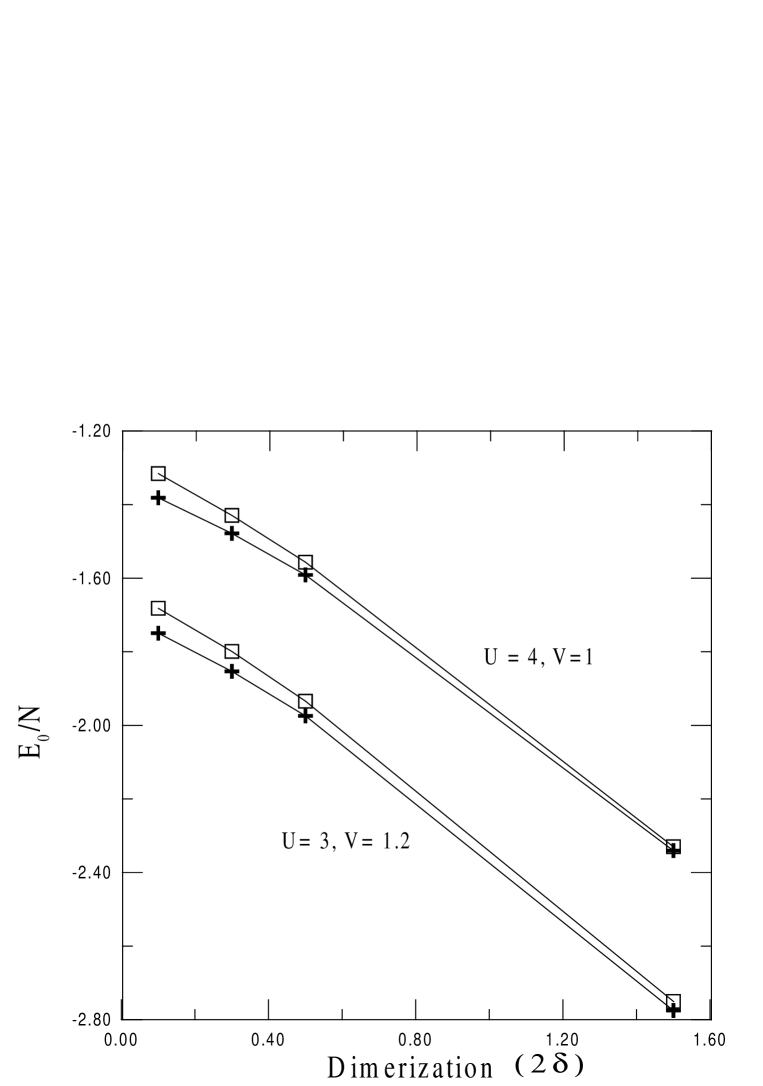
FIG. 1.: Ground state energies per site using the Matrix Product ansatz (blank square) compared with DMRG results (solid crosses) plotted against the degree of dimerization of the polymer chain and for several values of the PPP parameters U and V in equation (28).

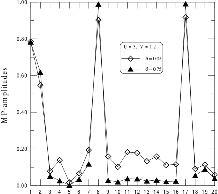
FIG. 2.: Absolute value of the twenty independent variational parameters used in the Matrix Product ansatz using six block bulk states.

State	$m$	$h$	$2S^{z}$	${m}_{J}$	$\eta^{J}_{m}$	$m_{P}$	$\eta^{P}_{m}$
$\bullet-\bullet$	1	0	0	1	1	1	1
$\times\circ+\circ\times$	2	0	0	2	1	2	1
$\times\circ-\circ\times$	3	0	0	3	-1	3	1
$\uparrow\uparrow$	4	0	2	4	1	6	-1
$\uparrow\downarrow+\downarrow\uparrow$	5	0	0	5	1	5	-1
$\downarrow\downarrow$	6	0	-2	6	1	4	-1
$\circ\circ$	7	2	0	8	-1	7	-1
$\times\times$	8	-2	0	7	-1	8	-1
$\circ\uparrow+\uparrow\circ$	9	1	1	15	-1	10	-1
$\circ\downarrow+\downarrow\circ$	10	1	- 1	16	-1	9	-1
$\circ\uparrow-\uparrow\circ$	11	1	1	13	-1	12	-1
$\circ\downarrow-\downarrow\circ$	12	1	- 1	14	-1	11	-1
$\times\uparrow+\uparrow\times$	13	-1	1	11	1	14	1
$\times\downarrow+\downarrow\times$	14	-1	- 1	12	1	13	1
$\times\uparrow-\uparrow\times$	15	-1	1	9	1	16	1
$\times\downarrow-\downarrow\times$	16	-1	- 1	10	1	15	1

Table 1.- States forming the monomer basis of the MP ansatz. The states given in the first column have to be normalized. $\bullet-\bullet$ represents a singlet valence bond state, $\times$ represents a double occupied site, $\circ$ symbolizes an empty site and $\uparrow,\downarrow$ symbolizes singly occupied sites with spin up and down. $h$ denotes the excess or defect of holes as compared to the half filling situation. $2S^{z}$ is twice the third component of the spin. $m_{J}$ and $m_{P}$ are the states obtained upon applying the operators $\hat{J}$ and $\hat{P}$ on the monomer state $m$ defined in eqs. (10). $\eta^{J}_{m}$ and $\eta^{P}_{m}$ are the corresponding signs appearing in eqs.(13).

State	$\alpha$	$h$	$2S^{z}$	${\alpha}_{J}$	$\eta^{J}_{\alpha}$	$\alpha_{P}$	$\eta^{P}_{\alpha}$
$\bullet-\bullet$	1	0	0	1	1	1	1
$\times\circ-\circ\times$	2	0	0	2	-1	2	1
$\circ\uparrow+\uparrow\circ$	3	1	1	5	-1	4	-1
$\circ\downarrow+\downarrow\circ$	4	1	- 1	6	-1	3	-1
$\times\uparrow-\uparrow\times$	5	-1	1	3	1	6	1
$\times\downarrow-\downarrow\times$	6	-1	- 1	4	1	5	1

Table 2. The notations are as in table 1. The states appearing in the first column are for illustration purposes. They simply show the type of symmetry of the block state as compared with the monomer states defined in table 1.

$x_{i}$	$\alpha$	$m$	$\beta$	$x_{i}$	$\alpha$	$m$	$\beta$
$x_{1}$	1	1	1	$x_{11}$	3	1	3
$x_{2}$	1	2	1	$x_{12}$	3	2	3
$x_{3}$	1	3	2	$x_{13}$	3	3	3
$x_{4}$	1	9	6	$x_{14}$	3	4	4
$x_{5}$	1	11	6	$x_{15}$	3	5	3
$x_{6}$	2	1	2	$x_{16}$	3	7	5
$x_{7}$	2	2	2	$x_{17}$	3	9	1
$x_{8}$	2	3	1	$x_{18}$	3	9	2
$x_{9}$	2	9	6	$x_{19}$	3	11	1
$x_{10}$	2	11	6	$x_{20}$	3	11	2

Table 3. List of the variational parameters $x_{i}$ in terms of the MP-amplitudes $A_{\alpha,\beta}[m]$. The total of non vanishing amplitudes $A_{\alpha,\beta}[m]$ is 62. The remaining 42 amplitudes can be computed using eqs.(15).

REFERENCES

- [1] D. Baeriswyl, D.K. Campbell and S. Mazumdar, in Conjugated Conducting Polymers, edited by H. Kiess (Springer-Verlag, Heidelberg, 1992), pp 7-133.
- [2] E. Hückel, Z. Physik 76, 628 (1932).
- [3] W.P. Su, J.R. Schrieffer and A.J. Heeger, Phys. Rev B22, 2099 (1980).
- [4] T. Holstein, Ann. of Phys. 8, 325 (1959).
- [5] R. Pariser and R. G. Parr, J. Chem. Phys. 21 (1953) 446; J. A. Pople, Trans. Faraday Soc. 42 (1953) 1375.
- [6] R.G. Parr, The Quantum Teory of Molecular Electronic Structure, Benjamin, New York, 1958.
- [7] S.R. White, Phys. Rev. Lett. 69, 2863 (1992), Phys. Rev. B 48, 10345 (1993).
- [8] S. Ramashesa, S. K. Pati, H. R. Krishnamurthy, Z. Shuai and J.L. Bredas, Phys. Rev. B 54, 7598 (1996).
- [9] Z. Shuai, S.K. Pati, W.P. Su, J.L. Bredas and S. Ramasesha Phys. Rev. B 55 15368 (1997).
- [10] W. Barford and R.J. Bursill, Chem. Phys. Lett.268 535 (1997); Synth. Met. 85 1155 (1997). R. J. Bursill, C. Castleton and W. Barford, Chem. Phys. Lett. 294 305 (1998). M. Boman and R.J. Bursinll, Phys. Rev. B 57 15167 (1998).
- [11] D. Yaron, E.E. Moore, Z. Shuai, J.J. Bredas, J. Chem. Phys. 108, 7451 (1998).
- [12] G. Fano, F. Ortolani and L. Ziosi, J. Chem. Phys 108, 9246 (1998); J. Chem. Phys 110, 1277 (1999).
- [13] S. Pleutin and J.L. Fave, J. Phys. Cond. Matt. 10, 3941 (1998).
- [14] S. Pleutin, E. Jeckelman, M.A. Martin-Delgado and G. Sierra, preprint July 1999, cond-mat/9908062, to appear in Prog. Theo. Chem. Phys.
- [15] G. Sierra and M.A. Martin-Delgado, Phys. Rev. B 56, 8774 (1997). For a review on the RVA method see M.A. Martin-Delgado and G. Sierra in “Density Matrix Renormalization Group”, eds. I. Peschel et al. LNP vol. 528. Springer-Verlag, 1999.
- [16] M. Chandros, Y. Shimoi and S. Mazumdar, Phys. Rev. B 59, 4822 (1999).
- [17] A. Klumper, A. Schadschneider and Z. Zittartz, Europhys. Lett. 24, 293 (1993); S. Ostlund and S. Rommer, Phys. Rev. Lett. 75, 3537 (1995); S. Rommer and S. Ostlund, Phys. Rev. B 55, 2164 (1997).
- [18] J.M. Roman, G. Sierra, J. Dukelsky and M.A. Martin-Delgado, J. Phys. A: Math. Gen. 31, 9729 (1998).
- [19] W.T. Simpson, J. Am. Chem. Soc. 77, 6164 (1955).
- [20] Z. Shuai, J.L. Bredas, S.K. Pati and S. Ramashesa, Phys. Rev. B 56, 9298 (1997).
- [21] J. Dukelsky, M.A. Martin-Delgado, T. Nishino and G. Sierra, Europhys. Lett. 43, 457 (1998).