Correlation functions in the two-dimensional
random-field Ising model

Abstract

Transfer-matrix methods are used to study the probability distributions of spin-spin correlation functions $G$ in the two-dimensional random-field Ising model, on long strips of width $L=3-15$ sites, for binary field distributions at generic distance $R$, temperature $T$ and field intensity $h_{0}$. For moderately high $T$, and $h_{0}$ of the order of magnitude used in most experiments, the distributions are singly-peaked, though rather asymmetric. For low temperatures the single-peaked shape deteriorates, crossing over towards a double-$\delta$ ground-state structure. A connection is obtained between the probability distribution for correlation functions and the underlying distribution of accumulated field fluctuations. Analytical expressions are in good agreement with numerical results for $R/L\gtrsim 1$, low $T$, $h_{0}$ not too small, and near $G=1$. From a finite-size ansatz at $T=T_{c}(h_{0}=0)$, $h_{0}\to 0$, averaged correlation functions are predicted to scale with $L^{y}h_{0}$, $y=7/8$. From numerical data we estimate $y=0.875\pm 0.025$, in excellent agreement with theory. In the same region, the RMS relative width $W$ of the probability distributions varies for fixed $R/L=1$ as $W\sim h_{0}^{\kappa}\,f(L\,h_{0}^{u})$ with $\kappa\simeq 0.45$, $u\simeq 0.8$ ; $f(x)$ appears to saturate when $x\to\infty$, thus implying $W\sim h_{0}^{\kappa}$ in $d=2$.

]

I Introduction

It is by now well established that the space dimensionality $d=2$ is the lower critical dimension of the random field Ising model (RFIM) [1, 2, 3], in agreement with the early domain-wall picture of Imry and Ma [4]. Thus, as usual for a borderline dimensionality, details of two-dimensional behaviour are rather intricate. The divergence of the low-temperature correlation length as the field intensity approaches zero is apparently anomalously severe [5]. This is at least partly responsible for difficulties encountered in the application of normally very powerful numerical techniques to this problem. In particular, transfer-matrix (TM) methods have been used, either for fully finite [6, 7, 8] or semi-infinite [9] geometries. TM calculations have usually focused upon the structure factor, as obtained from suitable derivatives of the partition function. The correlation length is then derived from the structure factor, under assumption of specific scaling forms [7, 8, 9]; results thus far have been at least in qualitative agreement with theoretical predictions [5].

Many recent studies of the RFIM, both in $d=2$ and 3, have concentrated on zero-temperature properties, as an exact ground-state algorithm first applied some time ago [10] has been revisited [11, 12]. In our earlier work [13, 14], where a domain-wall scaling picture was developed for bar-like systems in general $d$, numerical support for theory was provided in $d=2$, $T=0$ by a version of such algorithm adapted to strip geometries. For $T\neq 0$ we relied on a TM treatment of the free energy, again on strips.

Here we deal directly with probability distributions of spin-spin correlation functions, calculated by TM methods on semi-infinite (strip) systems. Interest in probability distribution functions has increased recently, regarding extensive quantities in critical disordered systems. This is in line with the growing realisation that lack of self-averaging tends to be the rule, rather than the exception, e.g. for susceptibilities and magnetisations in such systems [15], implying that the width of the associated probability distributions is a permanent feature that does not trivially vanish with increasing sample size. In the present case, lack of self-averaging does not come as a surprise, as correlation functions are not extensive [16], so the usual Brout argument [17] is not expected to apply. Also, in $d=2$ the random field moves the second-order transition to $T=0$, so the $d=2$ RFIM is off criticality at any $T\geq 0$; experimental manifestations of microscopic features of the $d=2$ RFIM come indirectly through (sample-averaged) non-critical properties [18, 19, 20]. Indeed, consideration of the crossover behaviour in the vicinity of the zero-field, pure-Ising, critical point provides interesting information, as shown in Section IV .

In what follows, we first discuss the ranges of spin-spin distance $R$, temperature $T$ and random-field intensity $h_{0}$ for which the statistics of correlation functions display the most interesting features, and illustrate our choices with simple examples. We then turn to the connection between field– and correlation-function distributions, and show how, in suitable limits, one can extract the latter from the former. Next we study the line $T=T_{c}(h_{0}=0),h_{0}\to 0$, and use correlation functions to extract information on scaling behaviour corresponding to the destruction of long-range order by the field. A final section summarizes our work.

II Numerical techniques and parameter ranges

We calculate the spin-spin correlation function $G(R)\equiv\langle\sigma_{0}^{1}\sigma_{R}^{1}\rangle$, between spins on the same row (say, row 1), and $R$ columns apart, of strips of a square lattice of ferromagnetic Ising spins with nearest-neighbour interaction $J=1$, of width $3\leq L\leq 15$ sites with periodic boundary conditions across. This is done along the lines of Sec. 1.4 of Ref. [21], with standard adaptations for an inhomogeneous system [22]. The strip widths used are those manageable on standard workstations, without unusually large memory or time requirements; as the main overall advantage of TM calculations (against e.g. those on fully finite, $L\times L$ systems), is that monotonic trends set in for relatively small strip widths [21], the upper bound on $L$ does not significantly constrain our analysis. It does, however, matter for the values of $R$ used, since the interesting range of $R/L$ is around one, where the transition between $d=1$ and $d=2$ behaviour takes place.

Different sorts of averaging are involved in this case. For a given realisation of the site-dependent random fields, one has (for sufficiently low field intensity) a macroscopic ground-state degeneracy [11]. TM methods take into account the Boltzmann weights of all possible spin configurations, so they scan the whole set of available ground states for a given realisation of quenched disorder. One must then promediate over many such realisations, which is done as follows. At each iteration of the TM from one column to the next, the random-field values $h$ are drawn for each site from the binary distribution:

$$P(h)={1\over 2}[\,\delta(h-h_{0})+\delta(h+h_{0})\,]\ \ .$$ (1)

By shifting the origin along the strip and accumulating the respective results, one can produce normalized histograms, $P(G)$, of occurrence of $G(R)$. With typical strip lengths $N=10^{6}$ columns, we generate $10^{4}-10^{5}$ independent estimates of $G(R)$ for $R$ in the range $5-15$ which corresponds to $R/L\sim 1$, as explained above.

In our previous study of the unfrustrated random-bond Ising model [23], the probability distribution function of correlations was expected to be log-normal for strictly one-dimensional systems [16]. This led us to a picture where, for strip width $L$ and spin-spin distance $R$, the distribution would evolve perturbatively away from log-normal with increasing $L/R$. Thus, there we used logarithmic binning for the histograms of occurrence of $G(R)$: a convenient interval of variation of $\ln G(R)$ was divided into, usually, $10^{3}$ bins, each particular realization being assigned to the appropriate bin. As a similar starting point is not available here, and negative values of correlations may occur, we have resorted to a simple linear choice, dividing the whole $[-1,1]$ interval of variation of $G(R)$ into (again, usually $10^{3}$) equal bins.

The temperature and field intervals of interest are broadly circumscribed because spin-spin correlations are induced by the ferromagnetic (unit) interaction. Thus one must keep to values of $T$ and $h_{0}$ that are not sufficient to render the coupling negligible; rough boundaries, to be refined next, are $T_{c}(h_{0}=0)=2.269\dots$ and $h_{0c}(T=0)=4$ (above this latter value each spin always obeys the local field).

We have found $T_{low}=0.6$ to be low enough to display ground-state effects rather prominently. Recall that strictly at $T=0$ correlation-function histograms are trivial double–$\delta$ peaks at $G(R)=\pm 1$; this reflects the frozen-domain structure of the ground state, which is best investigated directly as done by others [11, 12]. Conversely, here we wished to investigate departures from the double-$\delta$ shape, induced by increasing $T$. On the other hand, $T_{high}=2.0$ is high enough so that field fluctuations (in the range of $h_{0}$ spelt out in the next paragraph) have mainly a perturbative effect.

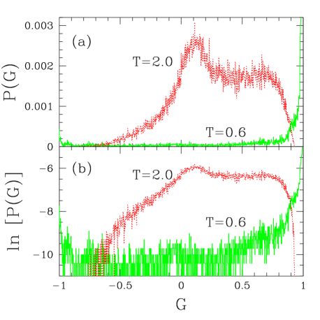
FIG. 1.: Normalized histograms $P(G)$ of occurrence of $G$ for strip width $L=5$, length $N=10^{6}$ columns, $R=15$, $h_{0}=0.5$, and $T=0.6$ and $2.0$. Binwidth $2\times 10^{-3}$. Vertical axis has linear scale in (a) and logarithmic in (b), the latter in order to emphasize values occurring with low frequencies.

Experimental studies [18, 19, 20] of $d=2$ dilute Ising antiferromagnets in a uniform field $H$ (argued by Fishman and Aharony [24] to be equivalent to the RFIM) concentrate on $H$-values corresponding to $h_{0}\lesssim 0.1-0.2$ in Eq. (1), enough to cause significant departures from zero-field behaviour. Higher fields $h_{0}\gtrsim 1$ are convenient to enrich domain statistics in simulations of fully finite systems, as they reduce low-temperature domain sizes and increase degeneracy [11, 12]. However, already for $h_{0}=0.5$ the histograms of correlation functions were found to be utterly distorted (compared to a paradigm of single-peaked structures with reasonably-defined widths), so as to be intractable in terms of a simple description with few parameters. This echoes the experimental observation for Rb₂C_0.7Mg_0.3F₄, that “…applied fields very much less than the Co²⁺ molecular fields … have quite drastic effects” [18]. Fig. 1 illustrates the point.

Nevertheless, for $h_{0}\lesssim 0.1-0.15$ and high $T$, the overall picture stays very close to that depicted in Fig. 2, with the following main features: (i) a clearly-identifiable single peak, below the zero-field value $G_{0}\equiv G(h_{0}=0)$; (ii) a short tail below the peak and a long one above it, such that (iii) all moments of order $\geq 0$ of the distribution are above $G_{0}$. In Figure 2 we show the zeroth ($\exp\langle\ln G\rangle$) and first ($\langle G\rangle$) moments.

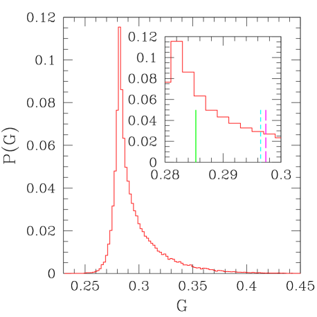
FIG. 2.: Normalized histogram $P(G)$ of occurrence of $G$ for strip width $L=5$, length $N=10^{6}$ columns, $R=15$, $h_{0}=0.05$ and $T=2.0$. Binwidth $2\times 10^{-3}$. Vertical bars in inset located respectively at: $G_{0}$ (full line); $\exp\langle\ln G\rangle$ (short-dashed); $\langle G\rangle$ (long-dashed).

This scenario breaks down for low temperatures, as $G(h_{0}=0)$ becomes close to the upper limit of unity, for $R/L\sim 1$ and the strip widths within reach. However, this latter regime can be understood in terms of a direct connection between field– and correlation-function distributions, described in Section III below.

For fixed $R$, small $h_{0}$ and high $T$, Figure 3 shows the typical evolution of distributions against $L$. Note that, with $h_{0}=0.15$, the single-peak structure shows early signs of fraying.

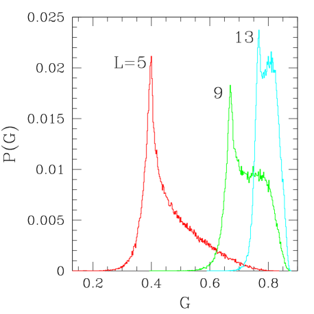
FIG. 3.: Normalized histograms $P(G)$ of occurrence of $G$ for strip widths $L=5$, $9$ and $13$; length $N=10^{6}$ columns, $R=10$, $h_{0}=0.15$ and $T=2.0$. Binwidth $2\times 10^{-3}$.

One can see in Figure 3 a narrowing effect with increasing $L$. This is quantitatively depicted in Figure 4, for which the use of $R/L$ on the horizontal axis is inspired in usual ideas of finite-size scaling, and has proven fruitful in our earlier study of random-bond systems [23].

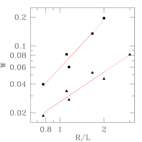
FIG. 4.: Double-logarithmic plot of RMS relative widths $W$ of distributions against $R/L$. Strip widths $L=5$, 9, 13; $R=10$, 15; $h_{0}=0.05$ (triangles) and 0.15 (squares). Straight lines are least-squares fits to each set of data (see text). $T=2.0$.

Though the RMS relative width $W\equiv(\langle G^{2}\rangle-\langle G\rangle^{2})^{1/2}/\langle G\rangle$ appears to approach zero for small $R/L$ (where, as argued in Ref. [23], $d=2$ behaviour should show up), we note that: (i) the data display non-monotonic jumps even for fixed $h_{0}$; and (ii) power-law fits of $W$ against $(R/L)^{x}$ show a rather strong dependence of $x$ on $h_{0}$ (for data in Figure 4 one has $x\simeq 1$ for $h_{0}=0.05$, and $2$ for $h_{0}=0.15)$. These facts indicate that, from consideration of the above data alone, we are not in a position to conclude that $W\to 0$ as the true $d=2$ regime is approached. Indeed, in Section IV below a different analysis, at fixed $R/L$, strongly suggests that the widths do not vanish in the two-dimensional limit.

III Distribution of $G$ from field distribution

An important question is how the field distribution gives rise to the distribution for the correlation function $G(R)\equiv\langle\sigma_{0}\sigma_{R}\rangle$ (at specific separation $R$).

A scenario worth exploring is the following: the probability distribution $P(G)$ for $G(R)$ arises from a distribution of characteristic scales $\xi$, related to $G(R)$ via $G(R)\sim\exp(-R/\xi)$, with $\xi$ distributed according to some distribution. This last probability distribution has then to be related to the field distribution. At low temperatures a domain picture might provide that relationship: a distribution of domain sizes $\xi_{i}$ arises from the distribution of fields aggregated over each domain, e.g. by minimising energy (or free energy) along the lines of Ref. [13], but generalised to consider specific field configurations, with their associated probability (the free energy minimisation may make such an approach applicable up to temperatures of order $T_{c}(h=0)$ ).

The simplest such scheme uses a common domain size $\xi$, over which the total field is $h=xh_{0}\sqrt{\xi L}$ with $p(x)=e^{-x^{2}/2}/\sqrt{2\pi}$ . This is the distribution of aggregated fields on a domain, arising from the independent distributions ${1\over 2}[\delta(h-h_{0})+\delta(h+h_{0})]$ of fields $h_{i}$ at each site $i$.. Then minimising the free energy per unit length (for the $T=0$ problem) gives

$$\xi=\xi(x)={4J^{2}L\over x^{2}h_{0}^{2}}\ \ \ .$$ (2)

Hence, from the probability distribution $p(x)$, there arises a probability distribution for $\xi(x)$, and via that a probability distribution $P(G)$ for $G(R)\sim\exp(-R/\xi)$. The result is

$$P(G,T=0)=\left({2J^{2}L\over h_{0}^{2}R}\right)^{1/2}{1\over\sqrt{2\pi}}{G^{{2J^{2}L\over h_{0}^{2}R}-1}\over(\ln{1/G})^{1/2}}\ \ \ .$$ (3)

The important parameter in this zero-temperature description is $\lambda\equiv{2J^{2}L\over h_{0}^{2}R}$ (which is of order one for $R=15$, $L=5$, $h_{0}=0.5$, for example).

The $T\neq 0$ generalisation of such pictures involves the entropic contribution $-T(S_{0}+S_{1})$ to the free energy $F$, which includes a contribution from positioning of domain walls ($-TS_{0}$) (see Ref. [13], but still allowing for probabilities of specific field configurations) and also one from the random-walk-like wandering of the domain walls ($-TS_{1}$).

These entropies are (using the simplest picture of a single $\xi(x)$) $S_{0}=k_{B}\ln\xi(x)/\xi(x)$ (using reduction valid for $\xi(x)$ large), and $S_{1}=k_{B}\ln\mu^{L}/\xi(x)=k_{B}(L/\xi(x))\ln\mu$, with $\mu\sim z-1$, $z=$ lattice coordination number. Minimisation of $F$ per unit length then gives

$$0={h_{0}x\sqrt{L\xi}\over 2JL}-1+{k_{B}T\over JL}\left(L\ln\mu+\ln\xi-1\right)\ \ \ .$$ (4)

The variable $x$ is again distributed with the domain-aggregated field distribution $p(x)=e^{-x^{2}/2}/\sqrt{2\pi}$ which, via Equation (4) then provides the distribution of $\xi$ and finally the distribution for $G\sim e^{-R/\xi}$ (along the general lines indicated above). Different pairs of terms dominate Equation (4) in different regimes of $h_{0}$, $T$ and $L$. Of special interest to us are the first-order low-temperature corrections. An approximate treatment of Equation (4), valid for $G$ near 1, gives

$$P(G,T)\propto P(G,T=0)(\ln 1/G)^{-4k_{B}T/JL}\ \ \ ,$$ (5)

with $P(G,T=0)$ given by Equation (3). Apart from weakly $L$-dependent normalization factors, one should have

$$P^{\prime}(G)\equiv P(G,T)G^{-\alpha}(\ln(1/G))^{\beta}={\rm const}\ \ \ ,$$ (6)

where $\alpha\equiv(2J^{2}L/h_{0}^{2}R)-1$, $\beta\equiv 1/2+4k_{B}T/JL$ .

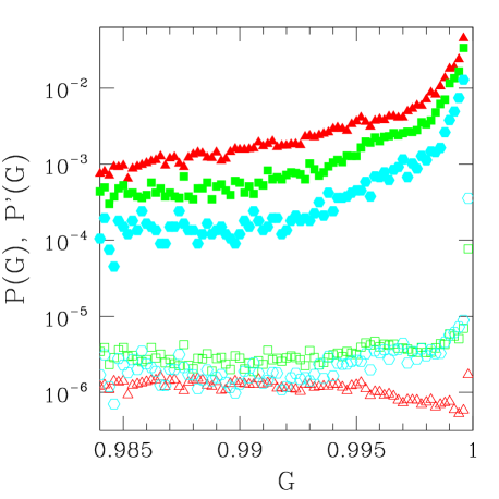
FIG. 5.: Histograms of occurrence of $G$ for $T=0.6$, $h_{0}=0.5$, $R=15$, near $G=1$; $L=3$ (triangles), $5$ (squares) and $7$ (hexagons). Binwidth $2\times 10^{-4}$. Full symbols: normalized histograms, $P(G)$. Empty symbols: $P^{\prime}(G)$, Eq. (6).

In Figure 5 we check Equation (6) for $T=0.6$, $h_{0}=0.5$, $R=15$ and $L=3$, 5 and 7. Use of narrow strips (i.e. $R/L>1$) and high fields is important in order to produce broad distributions in the low-temperature regime concerned. One sees that, indeed, the strong $G$– dependence of $P(G,T)$ near $G=1$ can be essentially accounted for by the factors in Equation (6).

IV Scaling near zero-field critical point

According to theory [5, 19, 20, 24, 25], the scaling behaviour of the RFIM depends on the variable $h_{0}^{2}|t|^{-\phi}$ where $h_{0}$ is the random-field intensity and $t=(T-T_{c}(h_{0}))/T_{c}(h_{0})$ is a reduced temperature. For $d>d_{c}=2$ $T_{c}(h_{0})$ is the field-dependent temperature at which a sharp transition still occurs; it turns out that even in $d=2$ the dominant terms still depend on the same combination, where now [20] “$T_{c}(h_{0})$” denotes a pseudo-critical temperature marking, e.g., the location of the rounded specific-heat peak. This is true except for the $d=2$ specific heat (which does not concern us directly here), where $\ln h_{0}$-dependent terms also play an important role [19, 26]. Further, it is predicted [25] that the crossover exponent $\phi=\gamma$, the pure Ising susceptibility exponent. In $d=2$, specific heat [19] and neutron-scattering [20] data are in good agreement both with the choice of scaling variable as above, and with the exactly known $\gamma=7/4$ .

Here we propose a direct check of scaling, as follows. For $h_{0}\to 0$, near $T_{c\,0}\equiv T_{c}(h_{0}=0)$, one expects [19] “$T_{c}(h_{0})$”$=T_{c\,0}-ch_{0}^{2/\phi}$. Hence, $h_{0}^{-2/\phi}t\simeq h_{0}^{-2/\phi}(T-T_{c\,0})$ apart from a small, finite shift. Setting $T=T_{c\,0}$ and making the usual finite-size scaling ansatz [27] $t\to L^{-1/\nu}$ with the pure Ising value $\nu=1$ (this latter assumption to be verified), one obtains that the (finite-size) scaling variable at $T=T_{c\,0}$ must be

$$x\equiv h_{0}L^{\phi/2\nu}\ ,\ \ \ (T=T_{c\,0},h_{0}\to 0)$$ (7)

with $\phi/2\nu=7/8$ in $d=2$. This implies that the correlation length related to the decay of ferromagnetic spin-spin correlations diverges along this particular line as

$$\xi(T=T_{c\,0},h_{0}\to 0)\sim h_{0}^{-1/y}\ ,\ \ \ y=\phi/2\nu.$$ (8)

From standard finite-size scaling [27], the correlation functions for distance $R$, strip width $L$, $t\equiv T-T_{c\,0}=0$ and random-field intensity $h_{0}$ are then expected to behave as

$$G(R,L,t=0,h_{0})=L^{-\eta}\,\Gamma(R/L,L^{y}h_{0})\ \ \ .$$ (9)

In Figure 6 we show, for fixed $R/L=1$, the scaling plot thus suggested, where $y$ has been adjusted to provide the best data collapse. The same procedures have been used very recently in studies of unfrustrated random-bond Potts models [28].

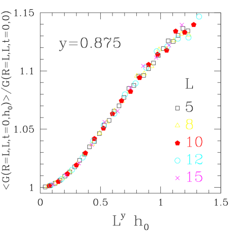
FIG. 6.: Averaged correlation functions (normalised by their zero-field counterparts) against $L^{y}\,h_{0}$ with $y=0.875$. Each point is the central estimate on a strip $N=10^{5}$ sites long. See text and Table I for a discussion of estimated error bars.

Note the use of averaged correlation functions, $\langle G\rangle$. We also performed plots with typical ones [23], $\exp(\langle\ln G\rangle)$, with entirely similar results. As remarked in Section II, one has $\langle G\rangle>G(h_{0}=0)$, on account of the long forward tail of the distribution. This happens for $\exp(\langle\ln G\rangle)$ as well, and is a scenario valid only for low field intensities. Near the end of the region where scaling holds, on the right of Figure 6, one indeed sees the beginning of a trend towards stabilization (which would, for higher fields, presumably turn into a decreasing function of $h_{0}$, were scaling still valid).

The value $y=0.875$ used in Figure 6 gave the best data collapse, which still kept reasonably good over the interval ($0.85,0.90$). The plots using $\exp(\langle\ln G\rangle)$ behaved in the same way. Thus our estimate is: $y=0.875\pm 0.025$ , in very good agreement with the finite-size scaling ansatz described above, with $\gamma=7/4$, $\nu=1$.

TABLE I.: Correlation functions calculated at $T=T_{c\,0}$, distance $R=L$ and random-field intensity $h_{0}=0$ ($G_{0}$) and $h_{0}=0.8L^{-7/8}$ ($\langle G(h_{0})\rangle$). Error bars in parentheses give uncertainties in last quoted digits, from spread among central estimates for five different runs on strips with $N=10^{5}$.

$L$	$G_{0}$	$\langle G(h_{0})\rangle$	$\langle G(h_{0})\rangle/G_{0}$
5	$0.333422277$	$0.36420(31)$	$1.0923(10)$
8	$0.300005458$	$0.32800(30)$	$1.0933(10)$
10	$0.284437852$	$0.31086(40)$	$1.0929(14)$
12	$0.272124932$	$0.29733(48)$	$1.0926(18)$
15	$0.257635774$	$0.28148(59)$	$1.0926(23)$

Each point in Figure 6 represents an average taken from one run on strips $N=10^{5}$ columns long. We now discuss the estimation of error bars, not shown in the Figure. Recalling that the width of the distributions is not expected to vanish in the thermodynamic limit, we follow the lines extensively elaborated elsewhere for similar cases [22, 23, 29], and estimate fluctuations by evaluating the spread among overall averages (i.e. central estimates) from different samples. For values of $L$ and $h_{0}$ such that $L^{7/8}h_{0}=0.8$ (approximately midway along the horizontal axis of Figure 6), we performed series of five runs, each with $N=10^{5}$, for each $L$. Table I shows the results. One sees that Equation (9) is satisfied to within 2 parts in $10^{3}$. Such an agreement is further evidence in suport of the scaling ansatz proposed above; it also suggests that the scaling power is $y=7/8$ exactly.

Incidentally, note that from the constancy against $L$ of the ratio $\langle G(R,L,t=0,h_{0})\rangle/G(R,L,t=0,0)$, as verified in Table I, and the scaling of correlation functions given in Equation (9), one immediately has $\eta=\eta_{Ising}=1/4$ for the decay of ferromagnetic correlations at $T=T_{c\,0}$, $h_{0}\to 0$ .

We now return to scaling of the RMS relative width $W$ of the distribution against field and strip width, restricting ourselves to $T$ near $T_{c\,0}$ and $h_{0}$ not very large. For fixed $R/L$, taking into account that the distribution broadens (a) with increasing random-field intensity (which is elementarily expected), and (b) also with increasing strip width (which we noticed in our numerics at $T=T_{c\,0}$), we propose the following scaling form:

$$W=h_{0}^{\kappa}\,f(L\,h_{0}^{u})\ \ \ ,$$ (10)

where the effective length $L_{h}\equiv h_{0}^{-u}$ plays the role of a saturation distance, such that $f(x)\to{\rm constant},x\gg 1$. In other words, (i) for high temperatures such as $T=T_{c\,0}$ and small $h_{0}$ there must be a regime in which the distribution remains recognizably similar to Figure 2, with the field-induced broadening reaching a relatively small maximum as $R$,$L\gg h_{0}^{-u}$ (at fixed $R/L$). At the other end $x\ll 1$, the only obvious constraint is that (ii) $f(x)$ must not increase faster than $x^{-\kappa/u}$ as $x\to 0$, if it does diverge at all.

From scaling plots of $W\,h_{0}^{-\kappa}$ against $L\,h_{0}^{u}$ (at $T=T_{c\,0}$ and $h_{0}$ not very large) with tentative values of the exponents, we have found the best data collapse to occur for $\kappa\simeq 0.43-0.50$ and $u\simeq 0.8$. Figure 7, where the vertical axis is logarithmic, shows our results for $\kappa=0.45$ and $u=0.8$. For $x>1$, the fitting spline is the function $y=-0.3-5.3\exp(-1.57x)$, implying a limiting scaled width $W\,h_{0}^{-\kappa}=\exp(-0.3)=0.83$ , consistent with (i) above. For $x<1$ the fitting curve is given by $y=1.73\ln x-1.40$, in agreement with requisite (ii).

To our knowledge there is no structural relationship between the width exponents $\kappa$ and $u$, and the standard critical indices, such as the crossover exponent $\phi$ discussed above. Conversely, one would expect widths to behave similarly to the above picture even at $T\neq T_{c\,0}$, provided that one keeps to high temperatures and low field intensities. Most likely, asymptotic scaled widths will depend on $T$; a matter for further investigation is whether or not the numerical values of the exponents will also vary.

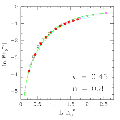
FIG. 7.: Semi-logarithmic scaling plot of RMS relative widths, $W\,h_{0}^{\kappa}$ against $L\,h_{0}^{u}$. Key to symbols is the same as in Figure 6. Curves are fitting splines (see text).

V conclusions

We have studied the probability distributions of occurrence of spin-spin correlation functions $G$ in the $d=2$ RFIM, for binary distributions of the local fields, at generic distance $R$, temperature $T$ and field intensity $h_{0}$, on long strips of width $L=3-15$ sites.

We have shown that for moderately high temperatures, of the order of the zero-field transition point $T_{c\,0}$, and field intensities $h_{0}\lesssim 0.1-0.2$ in units of the nearest-neighbour coupling (the same order of magnitude used in most experiments), the distributions retain a recognizable single-peaked structure, with a well-defined width. However, they display considerable asymmetry, with a short tail below the maximum and a long one above it, the latter owing to the mutual reinforcement between ferromagnetic spin-spin interactions and large accumulated-field fluctuations. For low temperatures the single-peaked shape deteriorates markedly, as crossover takes place towards the double-$\delta$ structure characteristic of the ground state.

We have established a connection between the probability distribution for correlation functions and the underlying distribution of accumulated field fluctuations. Starting from a zero-temperature description based on the distribution of (essentially flat) domain walls across the strip, we have shown how (low-) temperature effects can be incorporated, and proposed analytical expressions for the main dependence of the distribution of correlation functions on $R$, $L$, $T$ and $h_{0}$. In their assumed domain of validity, i.e. $R/L\gtrsim 1$, $T\ll 1$, not very small $h_{0}$, and close to the upper extreme $G=1$, they are in good quantitative agreement with numerically calculated distributions.

At $T=T_{c\,0}$, for $h_{0}\to 0$, we have made contact with scaling theory for bulk systems, and developed a finite-size ansatz to describe the scaling behaviour of averaged correlation functions. The variable that describes such behaviour was found to be $L^{y}h_{0}$, with $y=0.875\pm 0.025$ from numerical data, in excellent agreement with the ansatz’s prediction, $y=7/8$. In the same region, we have also studied the RMS relative width $W$ of the probability distributions, and found that, for fixed $R/L=1$ it varies as $W\sim h_{0}^{\kappa}\,f(L\,h_{0}^{u})$ with $\kappa\simeq 0.45$, $u\simeq 0.8$ . We have shown that $f(x)$ fits well to a saturating form when $x\to\infty$, thus implying $W\sim h_{0}^{\kappa}$ in $d=2$.

Further developments of the present work would include: (i) establishing analytical expressions to connect field fluctuations, domain size distribution and correlation function distributions in regimes such as $R/L\simeq 1$ (relevant to $d=2$ behaviour), $T\sim T_{c\,0}$, and valid for generic $G$; and (ii) a systematic study of the variation of widths and their associated exponents, both against temperature and the ratio $R/L$. We are currently considering such extensions.

Finally, as regards contact with experiment, one may ask how the present results for correlation functions relate e.g. to the wavevector-dependent scattering amplitudes in neutron scattering [18]. Attempts in this direction have been made earlier [9]. Since the scattering function reflects spatial averages over relatively extended regions, a connection to correlation functions must be established via a correlation length which represents the average decay of spin-spin correlations [9, 18]. Furthermore, fitting numerical data from one end to experimental results from the other is a tricky task, which is usually mediated by resorting to heuristically proposed line shapes. Of these, Lorentzian and Lorentzian-squared functions have been among the most popular [9, 18], though in principle there is no reason why one must be restricted to them. A broad range of possible line shapes, compounded with the wide variation exhibited by several properties of correlation functions, as shown in the present work, causes one to anticipate a fairly involved investigation.

- [1] J. Z. Imbrie, Phys. Rev. Lett. 53, 1747 (1984).
- [2] J. Bricmont and A. Kupiainen, Phys. Rev. Lett. 59, 1829 (1987).
- [3] M. Aizenman and J. Wehr, Phys. Rev. Lett. 62, 2503 (1989).
- [4] Y. Imry and S. Ma, Phys. Rev. Lett. 35, 1399 (1975).
- [5] A. Aharony and E. Pytte, Phys. Rev. B 27, 5872 (1983).
- [6] I. Morgenstern, K. Binder and R. M. Hornreich, Phys. Rev. B 23, 287 (1981).
- [7] E. Pytte and J. Fernandez, J. Appl. Phys. 57, 3274 (1985).
- [8] J. Fernandez, Phys. Rev. B 31, 2886 (1985).
- [9] U. Glaus, Phys. Rev. B 34, 3203 (1986).
- [10] A. Ogielski, Phys. Rev. Lett. 57, 1251 (1986).
- [11] J. Esser, U. Nowak and K. D. Usadel, Phys. Rev. B 55, 5866 (1997); S. Bastea and P. M. Duxbury, Phys. Rev. E58, 4261 (1998).
- [12] M. Alava and H. Rieger, Phys. Rev. E58, 4284 (1998); E. T. Seppälä, V. Petäjä, and M. J. Alava, ibid. 58, R5217 (1998); C. Frontera and E. Vives, ibid. 59, R1295 (1999).
- [13] R. B. Stinchcombe, E. D. Moore and S. L. A. de Queiroz, Europhys. Lett. 35, 295 (1996).
- [14] E. D. Moore, R. B. Stinchcombe, and S. L. A. de Queiroz, J. Phys. A 29, 7409 (1996).
- [15] S. Wiseman and E. Domany, Phys. Rev. E52, 3469 (1995); ibid. 58, 2938 (1998); A. Aharony and A. B. Harris, Phys. Rev. Lett.77, 3700 (1996). S. Wiseman and E. Domany, ibid. 81, 22 (1998); A. Aharony, A. B. Harris and S. Wiseman, ibid. 81, 252 (1998).
- [16] B. Derrida and H. Hilhorst, J. Phys. C 14, L539 (1981); B. Derrida, Phys. Rep. 103, 29 (1984).
- [17] R. Brout, Phys. Rev, 115, 824 (1959).
- [18] R. J. Birgeneau, H. Yoshizawa, R. A. Cowley, G. Shirane, and H. Ikeda, Phys. Rev. B28, 1438 (1983).
- [19] I. B. Ferreira, A. R. King, V. Jaccarino, J. L. Cardy, and H. J. Guggenheim, Phys. Rev. B28, 5192 (1983).
- [20] V. Jaccarino, A. R. King, and D. P. Belanger, J. Appl. Phys. 57, 3291 (1985); D. P Belanger, S. M. Rezende, A. R. King, and V. Jaccarino, ibid. 57, 3294 (1985); A. R. King, V. Jaccarino, M. Motokawa, K. Sugiyama, and M. Date, ibid. 57, 3297 (1985).
- [21] M. P. Nightingale, in Finite Size Scaling and Numerical Simulations of Statistical Systems, edited by V. Privman (World Scientific, Singapore, 1990).
- [22] S. L. A. de Queiroz, Phys. Rev. E51, 1030 (1995).
- [23] S. L. A. de Queiroz and R. B. Stinchcombe, Phys. Rev. E54, 190 (1996).
- [24] S. Fishman and A. Aharony, J. Phys. C 12, L729 (1979).
- [25] A. Aharony, Phys. Rev. B18, 3318 (1978).
- [26] T. Niemeijer and J.M.J. van Leeuwen, in Phase Transitions and Critical Phenomena, edited by C. Domb and M. S. Green (Academic, New York, 1976), Vol. 6.
- [27] M. N. Barber, in Phase Transitions and Critical Phenomena, edited by C. Domb and J. L. Lebowitz (Academic, New York, 1983), Vol. 8.
- [28] T. Olson and A. P. Young, cond-mat/9903068 .
- [29] F. D . A. Aarão Reis, S. L. A. de Queiroz and R. R. dos Santos, Phys. Rev. B54, R9616 (1996); ibid. 56, 6013 (1997).