The Recurrent Variational Approach applied to the Electronic Structure of Conjugated Polymers

Abstract

In this note, first the Recurrent Variational Approach (RVA) is introduced by using as example a non–trivial spin–model, the spin–1/2 antiferromagnetic two–leg–ladder. Then, a first application of this scheme to the electronic structure of conjugated polymers is proposed. An analogy between the two–leg ladder and the dimerized chain described by the Extended Peierls–Hubbard Hamiltonian is underlined and comparisons are made with DMRG calculations. The proposed ansatz is useful to get some analytical insight and it is a good starting point for further improvements using the RVA.

guessConjecture

1 Introduction

Conjugated molecules have attracted the attention of chemists and physicists since the early days of quantum mechanics. A remarkable example is given by Hückel who developed in the thirties the first independent–electron theory applicable to polyenes [Hückel (1931)]. In the sixties, J.A. Pople and S.H. Walmsley [Pople and Walmsley (1962)], introduced by using this simple theory in their pioneering work what would become twenty years later the solitonic excitations. Following this line, Su, Schrieffer, Heeger and, independently, Rice, proposed a model specifically devoted to the polyacetylene – known as the SSH model – where the role of the electron–phonon interaction is especially emphasized [Su (1979), Rice (1979)]; here, the polyacetylene is thought of as a Peierls insulator and the solitons, polarons and bipolarons as the major relevant excitations in this system. A very nice review of these early studies is included in the book of L. Salem [Salem (1966)] and a review about the SSH model can be found in the next reference [Heeger (1988)].

As a counterpart to this one–electron theory, the major role of electron correlation was soon recognized. In the fifties, the celebrated Pariser–Parr–Pople (PPP) Hamiltonian was suggested as a possible candidate for the studies of conjugated oligomers [Pariser and Parr (1953), Pople (1953)]. Later, Ovchinnikov et al. suggested to consider conjugated polymers as Mott–Hubbard instead of Peierls insulators [Ovchinnikov (1973)]. Then, one has to face a N–body problem with a strong Coulomb interaction with a non–zero range; it was subject to many numerical works such as exact diagonalizations of very small oligomers [Chandross (1999)], selected CI calculations [Tavan and Schulten (1987)] and, quite recently, Density Matrix Renormalization Group studies [Bendazzoli (1999), Boman and Bursill (1998), Jeckelmann (1998), Shuai (1998)]. The PPP Hamiltonian was also a preferential model to support the development of new methods before applying them to more realistic models; a very good example of such work is given by the Coupled–Cluster method first implemented in quantum chemistry for the PPP Hamiltonian [Cizek and Paldus (1971)].

Today, it is well recognized that both the electron–phonon and electron–electron interactions are equally important [Baeriswyl (1992)]. Moreover, interchain interaction and disorder are also of importance. Therefore, the problems one has to face to fully understand conjugated polymers stay quite challenging as it is the case for most of the recent organic compounds including high Tc superconductors. Despite a large amount of work, from the early thirties to now, the main questions remain awaiting an answer! For instance, a comprehensive picture for the ground state of these systems is still needed; it is the goal of this work to propose a relatively simple and, we believe, promising, way to understand the ground state of conjugated polymers.

More generally, one dimensional correlated electron systems appear over the years as a growing and important field in condensed matter theory. One main reason of that comes from the fact that these systems serve as a theoretical laboratory to explore new methods of solution, analytically or numerically. A second main reason – we would say more physical – comes from the fact that over the years, more and more experimental realisations of these systems appear. New concepts emerge from such studies as the ones included in the phenomenology of Luttinger–liquids [Haldane (1981)].

Among the technical methods proper to the one dimensional geometry, one may cite the Bethe ansatz [Bethe (1931)], the bosonization techniques [Haldane (1981)], and, more recently, the Density–Matrix Renormalization Group (DMRG) method [White (1993), Peschel (1999)] and a closely related scheme which is directly considered in this note, the Recurrent Variational Approach (RVA) [Sierra and Martín-Delgado (1997), Peschel (1999)]. The two first methods are analytical and the third one is numerical; the RVA method is in between.

The RVA, presented here, is a variational method invented recently in the context of spin–ladders [Sierra and Martín-Delgado (1997)]. It is a method very closely related to the DMRG scheme with the main differences coming from the fact that only one state is retained as the best candidate for the ground state in the RVA on the contrary to the DMRG which considered much more states [Peschel (1999)]. Most often, the results obtained with it are less accurate than the DMRG ones, but it is much easier to get a physical insight into the problem; the analysis of the results is simpler and the RVA could provide a ”physical” picture of some phenomena which, we believe, are of utmost importance in the field of conjugated polymers where the most important ingredient are still not fully recognized [Sariciftci (1997)].

This note is organized as follows. In section II, the RVA is presented using the example of the two–leg spin ladders. In section III, the RVA method is applied to the study of the dimerized chain described by the Extended Peierls–Hubbard model. A nice similarity between the two–leg ladder and this system is pointed out and comparisons with DMRG calculations are made. We conclude in section IV and give some reasonable perspectives.

2 RVA method applied to two–leg Spin Ladders

A spin ladder is an array of coupled spin chains. The horizontal chains are called the legs, the vertical ones, rungs. In the case of spin one–half antiferromagnet spin–ladders, these systems show a remarkable behaviour in function of the number of leg: there is a gap in the excitation spectrum of even–leg ladders and, on the contrary, no gap in the excitation spectrum of odd–leg ladders. In terms of correlation lengths, this means that there is short (long) –range spin correlation in even (odd) –leg ladder (see [Dagotto and Rice (1996)] for a review).

The even–leg ladders show a spin-liquid ground state described by a Resonance Valence Bond (RVB) state introduced by P.W. Anderson [Anderson (1987)]; such systems may be efficiently described by using a direct–space method as the DMRG and RVA ones. In this note, we will consider only the simplest even–leg ladder, the two–leg ladder, and we will describe it with the simplest RVB state, the Dimer–RVB state where the elementary singlets are between two nearest–neighbour sites. This problem is easily solved by using the RVA method [Sierra and Martín-Delgado (1997)]. Moreover, with the same scheme, it is possible straightforwardly to go beyond the simple Dimer–RVB state by considering more extended elementary singlets [Sierra and Martín-Delgado (1997)], and to study more complex systems as the four–leg ladders for instance [Roncaglia (1999)]. In principle, this method should be relevant for every one–dimensional system with exponentially decreasing correlation lengths as conjugated polymers [Pleutin (1999)].

In this note we consider the simplest case given by the two–leg ladder (see figure (1)). The corresponding Hamiltonian is the following

$$H=J\sum_{k=1}^{N-1}({\bf S}_{k}\cdot{\bf S}_{\overline{k+1}}+{\bf S}_{k+1}\cdot{\bf S}_{\overline{k}})+J^{\prime}\sum_{k=1}^{N}{\bf S}_{k}\cdot{\bf S}_{\overline{k}}$$ (1)

where $J$ ($J^{\prime}$) are the exchange integral for the leg (rung) with $J>0$ ($J^{\prime}>0$). $N$ denotes the number of rungs of the ladder and open periodic boundary conditions have been assumed.

Figure 1: The two–leg ladder with an AF–Heisenberg model described by two coupling constants: $J$ for the links in the legs, and $J^{\prime}$ for the vertical rungs

In the limit where $J^{\prime}$ is much larger than $J$, the ground state of (1) is simply given by the product of singlets localized along the rungs (see fig. (3)). Starting from this limit, one may include fluctuations around it to treat the general case described by the Hamiltonian (1). A minimal way to do it, is to consider instead of singlet on rungs, pairs of nearest neighbour singlets on the leg; these local fluctuations are called resonon in the rest of the paper. Therefore, the resonance mechanism – in the sense of Pauling [Pauling (1960)] – we will consider in the following are represented in figure (2).

Figure 2: The basic bond resonance mechanism between horizontal and vertical bonds in an elementary plaquette of four sites.

With the two selected local configurations, the singlet localized on a rung and the resonon, we have to generate the corresponding Hilbert space; the configurations are characterized by the number of resonon, $M$, and their positions, $\{x_{i}\}$, as it is shown in the next examples. The Hilbert space is splitted according to the number of resonon; we have then to consider

• the zero–resonon sector with one unique state $|0\rangle$ (Fig. 3),

  

  Figure 3: The zero–resonon state $|0\rangle$ in a two–leg ladder. It is made of all vertical rung singlets. It is the reference state in the strong coupling limit $J^{\prime}\gg J$.

• the one–resonon sector with the states $\{|x_{1}\rangle\}$ (Fig. 4),

  

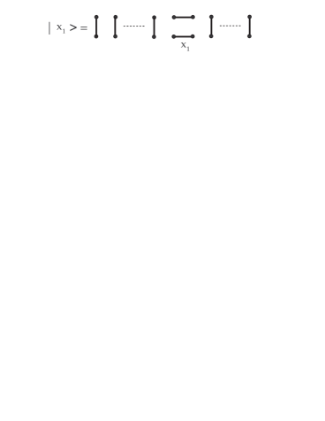
  Figure 4: A generic one–resonon state $|x_{1}\rangle$ in a two–leg ladder.

• the two–resonon sector with the states $\{|x_{1},x_{2}\rangle\}$ (Fig. 5),

  

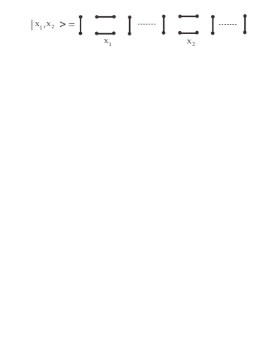
  Figure 5: A generic two–resonon state $|x_{1},x_{2}\rangle$ in a two–leg ladder.

  etc…

• the ${N\over 2}$–resonon sector with one unique state $|x_{1},x_{2},\ldots,x_{M}\rangle$ (Fig. 6).

  

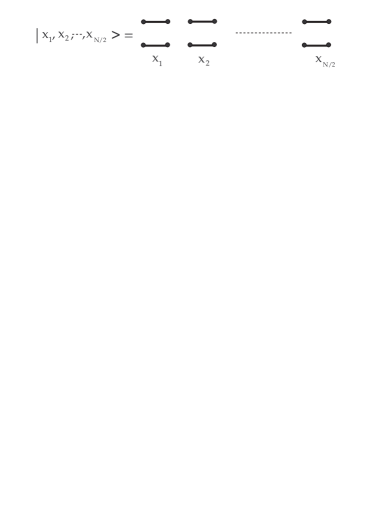
  Figure 6: The all–resonon state $|x_{1},x_{2},\ldots,x_{{N\over 2}}\rangle$ in a two–leg ladder.

With this classification of states we may write the following generalized Dimer–RVB state for a two–leg spin ladder,

$$|\psi(u)\rangle_{RVB}=\sum_{M=0}^{[N/2]}u^{M}\sum_{\{x_{1},x_{2},\ldots,x_{{M}}\}}|x_{1},x_{2},\ldots,x_{M}\rangle$$ (2)

where the sum is taken over all sectors with $M$ resonons and $u$ is the amplitude for a resonon. Here $u$ is a variational parameter to be determined upon minimization of the ground–state energy. As a result, it is a function of the ratio of couplings, namely, $u=u(J/J^{\prime})$.

Since we kept only two very localized building blocks, it is possible to generate the state (2) in a recursive manner which we present now.

2.1 Recurrence relations for the wave function

Denoting by $|N\rangle\equiv|\psi(u)\rangle_{RVB}$ a generic RVB state (2) for a two–leg ladder of $N$ rungs, there are only two possibilities or movements to create generic RVB states of higher length, namely,

• addition of one vertical rung to create the state $|N+1\rangle$,

• addition of one pair of horizontal bonds (resonon) to create $|N+2\rangle$.

From these arguments we can establish that the Dimer–RVB states (2) satisfy a recursion relation given by,

$$|N+2\rangle=|N+1\rangle\otimes|\phi_{1}\rangle_{N+2}+u\;|N\rangle\otimes|\phi_{2}\rangle_{N+1,N+2}$$ (3)

where the state denoted by $|\phi_{1}\rangle_{N+2}$ is a vertical rung at position $N+2$ and $|\phi_{2}\rangle_{N+1,N+2}$ is made up of a pair of horizontal bonds located between the rungs at $(N+1,N+2)$, i.e.,

$$|\phi_{2}\rangle_{N+1,N+2}=(N+1,\overline{N+2})(N+2,\overline{N+1})$$ (4)

where $(N,\overline{M})$ denotes a singlet between the sites $N$ and $\overline{M}$.

Using (3) one can generate recursively the Dimer RVB state $|N\rangle$ from previous states with lower length and estimate variationally the ground–state energy as,

$$e^{(g.s.)}_{N}\equiv{\langle N|H_{AFM}^{{two-leg}}|N\rangle\over(2N)\langle N|N\rangle}=e(N,J^{\prime}/J;u)$$ (5)

The value of $u$ is fixed by minimization of (5).

2.2 Recurrence relation for the norm

To compute the norms of the states (2) let us define

$$Z_{N}=\langle N|N\rangle$$ (6)

The two selected local configurations are not orthogonal, it is then convenient to define an auxiliary function $Y_{N}$ as follows,

$$Y_{N}=\big{(}_{N}\!\langle\phi_{1}|\otimes\langle N-1|\big{)}|N\rangle$$ (7)

The second order RR’s for the states leads (3) to a closed set of RR’s for the overlaps $Z_{N},Y_{N}$ , namely,

$$\begin{array}[]{rl}Z_{N+2}=&Z_{N+1}+uY_{N+1}+u^{2}Z_{N}\\ Y_{N+2}=&Z_{N+1}+{u\over 2}Y_{N+1}\end{array}$$ (8)

where we have made use of the result,

$${}_{N+1}\langle\phi_{1}|\phi_{2}\rangle_{N,N+1}={1\over 2}|\phi_{1}\rangle_{N}$$ (9)

The RR’s (8) together with the initial conditions,

$$\begin{array}[]{ll}Z_{0}=Z_{1}=1&\;,Y_{0}=0,\ Y_{1}=1\end{array}$$ (10)

determine $Z_{N}$ and $Y_{N}$ for arbitrary values of $N$ as functions of $u$.

Note that instead of introducing the function $Y_{N}$, it is also possible to make first linear combination of our building blocks, making used of (9) [Eder (1999)], in order to guaranty the orthogonality between the selected local configurations. The overlap would then be given by only one recurrent relation as it will be the case in the next section.

2.3 Recurrence relation for the expectation value of the Hamiltonian

The expectation values of the Hamiltonian can be determined following the same steps outlined above. To this end, we introduce the quantities,

$$\begin{array}[]{ll}E_{N}=\langle N|H_{N}|N\rangle&\;,D_{N}=\big{(}_{N}\!\langle\phi_{1}|\otimes\langle N-1|\big{)}H_{N}|N\rangle\end{array}$$ (11)

To obtain the RR’s satisfied by $E_{N},D_{N}$, one splits the Hamiltonian $H_{N}$ of a two–leg ladder of length $N$ (1) into two pieces:

$$H_{N}=H_{N-1}+H_{N-1,N}$$ (12)

where $H_{N-1}$ is the Hamiltonian of length $N-1$ and $H_{N-1,N}$ is the rest of the whole $H_{N}$ Hamiltonian, $H_{N-1,N}\equiv H_{N}-H_{N-1}$, which is made of one vertical rung and two horizontal links. With this splitting and using (3) and (6), we obtain,

$$\begin{array}[]{cl}E_{N+2}=&E_{N+1}+J^{\prime}\epsilon_{0}Z_{N+1}+u(D_{N+1}+(2J+J^{\prime})\epsilon_{0}Y_{N+1})\\ &+u^{2}(E_{N}+2J\epsilon_{0}Z_{N})\\ D_{N+2}=&E_{N+1}+J^{\prime}\epsilon_{0}Z_{N+1}+{u\over 2}(D_{N+1}+(2J+J^{\prime})\epsilon_{0}Y_{N+1})\end{array}$$ (13)

where $\epsilon_{0}=-3/4$ is the lowest eigenvalue of the operator ${\bf S}_{1}\cdot{\bf S}_{2}$.

The initial conditions for $E_{N}$ and $D_{N}$ are

$$\begin{array}[]{ll}E_{0}=0,\ E_{1}=J^{\prime}\epsilon_{0}&D_{0}=0,\ D_{1}=J^{\prime}\epsilon_{0}.\end{array}$$ (14)

The RR’s for the energies involve the norms of the states and depend both on $u$ and the coupling constants $J^{\prime},J$.

By working with orthogonal building blocks [Eder (1999)], it is also possible to go back to only one recurrent equation for the expectation value as for the norm; this will be the case in section 3.

2.4 Results for the Variational Ground–State Energy

The ground–state energy for a ladder of length $N$ is estimated. In the thermodynamic limit $N\rightarrow\infty$ one can find a closed expression for the density energy per site [Sierra and Martín-Delgado (1997)],

$$e_{\infty}=\lim_{N\rightarrow\infty}\frac{1}{2N}\frac{E_{N}}{Z_{N}}=\frac{R(\alpha)}{2\alpha Q^{\prime}(\alpha)P(\alpha)}$$ (15)

in terms of three polynomials $P,Q,R$ evaluated at the biggest root $\alpha$ of the cubic polynomial $Q(y)$. Finally one looks for the absolute minimum of $e_{\infty}$ by varying the parameter $u$. In Table 1 we show the ground–state energies per site for different values of the coupling constant ratio $J/J^{\prime}$, varying through strong, intermediate and weak coupling regimes.

Table 1: The values $-e_{\infty}^{{\rm MF}}/J^{\prime}$ are mean field (MF) values taken from [Gopalan (1994)], while $-e_{\infty}^{{\rm Lan}}/J^{\prime}$ are Lanczos values taken from [Barnes (1993)].

$J/J^{\prime}$	$u$	$-e_{\infty}^{{\rm RVA}}/J^{\prime}$	$-e_{\infty}^{{\rm MF}}/J^{\prime}$	$-e_{\infty}^{{\rm Lan}}/J^{\prime}$
$0$	$0$	$0.375$	$0.375000$
$0.2$	$0.128521$	$0.383114$	$0.382548$
$0.4$	$0.323211$	$0.40835$	$0.405430$
$0.6$	$0.578928$	$0.44853$	$0.442424$
$0.8$	$0.87441$	$0.499295$	$0.489552$
$1$	$1.18798$	$0.556958$	$0.542848$	$0.578$
$1.25$	$1.58519$	$0.63518$	$0.614473$	$0.6687$
$1.66$	$2.21853$	$0.772172$	$0.738360$	$0.8333$
$2.5$	$3.39153$	$1.06915$	$1.002856$	$1.18$
$5$	$5.9777$	$1.99285$		$2.265$

In the strong coupling regime $J/J^{\prime}<1$ the RVA states give a slightly better ground–state energy than the mean field result. This latter state produces rather unphysical results for $J/J^{\prime}>1$, which does not occur in our case. The RVA results compare also well with the exact results for $J^{\prime}\sim J$.

The RR’s can also be used to compute the spin correlator $\langle{\bf S}_{i}\cdot{\bf S}_{j}\rangle$ which has an exponential decay behaviour ${\rm exp}(-|i-j|/\xi)$, with $\xi$ the spin correlation length which satisfies the equation

$$u^{3}{\cal L}^{3}-(2+u)u^{2}{\cal L}^{2}-(2+4u)u^{2}{\cal L}+4u^{3}=0$$ (16)

where ${\cal L}={\rm e}^{1/\xi}$. For $J=J^{\prime}$ one finds $\xi=0.737$, which can be compared with its exact value given by 3.2. The latter results imply that at the isotropic point the bonds extended over three rungs are quite important. The simplest improvement of the Dimer–RVB state is to add a bond of length $\sqrt{5}$, analogue to a knight move, shown in figure (7); this first improvement leads to a third order RR. The ground state energy per site of this state is given by -0.5713 while the spin correlation length is 0.959. Hence there is an improvement in both quantities but still one needs longer bonds.

Figure 7: Local configurations extended over three rungs (the knight move)

Table 2: Here $m$ is total the number of multiplets, $N_{A}$ is the number of independent variational parameters, $d_{J}$ is the number of multiplets with spin $J$, $e_{\infty}^{{\rm MP},{\rm DMRG}}$ is the g.s. energy density of the matrix–product state (DMRG), $1-P_{m}$ is the probability of the states truncated out in the DMRG and $\xi^{\rm MP}$ is the spin correlation length of the MP state. The exact results are given by $e_{\infty}=1.4014845$ and $\xi=6.03$ [White and Huse (1993)].

$m$		$N_{A}$	$d_{1/2}$	$d_{3/2}$	$d_{5/2}$	$-e_{\infty}^{\rm MP}$		$-e_{\infty}^{\rm DMRG}$		$1-P_{m}$		$\xi^{\rm MP}$
$1$		$0$	$1$	$0$	$0$	$1.333333$		$1.333333$		$1.6\times 10^{-2}$		0.910
$2$		$2$	$1$	$1$	$0$	$1.399659$		$1.369077$		$1.4\times 10^{-3}$		2.600
$3$		$4$	$2$	$1$	$0$	$1.401093$		$1.392515$		$1.3\times 10^{-5}$		3.338
$4$		$7$	$2$	$2$	$0$	$1.401380$		$1.401380$		$1.6\times 10^{-5}$		3.937
$5$		$10$	$2$	$2$	$1$	$1.401443$		$1.401436$		$7.6\times 10^{-6}$		4.085
$6$		$13$	$2$	$3$	$1$	$1.401474$		$1.401468$		$1.3\times 10^{-6}$		4.453

The RVA method has already been applied to several model systems: to the Heisenberg two–leg ladder as we have seen above [Sierra and Martín-Delgado (1997)] and to two generalizations of it, the t-J [Sierra (1998)] and the Hubbard [Kim (1999)] two–leg ladders where the t-J and the Hubbard Hamiltonian, respectively, are defined on the lattice represented in the figure (1); it has been also applied to other ladders, the four–leg ladder [Roncaglia (1999)] and the diagonal ladders [Sierra (1999)], and to the spin–1 chain [Dukelsky (1998)]. In this latter case, very accurate calculations have been made by considering several local configurations (instead of our two retained here); the results are compared with Density Matrix Renormalization Group (DMRG) calculations [White and Huse (1993)]. We see that, in any case, the comparison are very good and even sometimes the RVA method gives better results than the DMRG (see Table II). A more complete review about RVA can be found in the following reference [Peschel (1999)].

3 RVA method applied to Conjugated Polymers

The low–energy properties of conjugated polymers involve $\pi$–electrons. Usually, they are described by the use of effective models as the well–known Pariser–Parr–Pople Hamiltonian [Pariser and Parr (1953), Pople (1953)]. This model includes both electron–phonon interaction (semi–classically) and a long range Coulomb interaction. The characteristic values for each kind of energetic contribution, kinetic, electron–phonon and electron–electron terms are approximatively of the same order of magnitude [Baeriswyl (1992)]; in this regime, the study of the PPP Hamiltonian – or some other short versions of it – are really not obvious.

Compared to the previous model used in section (2), the spin 1/2 antiferromagnetic Heisenberg model for a two–leg ladder, the PPP – or related – model is much more complicated: the long–range part of the Coulomb interaction is very difficult to treat and the dynamical variable are still not only spin but electron which involves spin and charge degree of freedom. However, due to the alternance between monomers, which can be large, and the link (the single bond) between the monomers, we will underline in this work a remarkable similarity between conjugated polymers and two–leg ladder. A similar wave function than (2) are proposed here for conjugated polymers - the rung of the ladder is played by the monomer and the resonon excitation of the two–leg ladder by a set of intermonomer fluctuations [Pleutin and Fave (1998), Pleutin (1999)]. We believe this wave function a natural and good starting point for further refinements.

We choose as model system the simplest conjugated polymers – the trans–polyacetylene. This compound shows a dimerized structure with an alternance between double bond (1.35Å) and single bond (1.45Å); the monomer is then simply a double bond (see figure (8)). The $\pi$ electrons are assumed to be effectively describe not by the full PPP Hamiltonian but by the Extended Peierls–Hubbard model (EPH) [Baeriswyl (1992), Jeckelmann (1998)], a short version of it, for simplicity

$$H=-\sum_{n,\sigma}(t-(-1)^{n}\frac{\Delta}{2})(c^{\dagger}_{n+1,\sigma}c^{\quad}_{n,\sigma}+c^{\dagger}_{n,\sigma}c^{\quad}_{n+1,\sigma})+U\sum_{n}n_{n\uparrow}n_{n\downarrow}+V\sum_{n}n_{n}n_{n+1}$$ (17)

The operator $c^{\dagger}_{n,\sigma}$ ($c^{\quad}_{n,\sigma}$) creates (annihilates) an electron of spin $\sigma$ at site $n$, $n_{n\sigma}=c^{\dagger}_{n,\sigma}c^{\quad}_{n,\sigma}$ and $n_{n}=n_{n\uparrow}+n_{n\downarrow}$. $t$ is the nearest–neighbour hopping term without dimerization, $\Delta$ is the usual dimerization order parameter, $U$ is the on-site Hubbard repulsion and $V$ is the nearest–neighbour charge density – charge density interaction. We will note in the following for convenience, $t_{d}=t+\frac{\Delta}{2}$ and $t_{s}=t-\frac{\Delta}{2}$, the hopping term for the double and the single bond respectively.

Figure 8: Model for the trans–polyacetylene and the system of bonding – antibonding levels associated with each double–bond

Because of the dimerization, the one electron density is more pronounced on the double bonds than on the single bonds; this is more and more apparent when the dimerization increases. More generally, this is the case for every conjugated polymers where the one–electron density is peaked on the monomer region. In this sense, conjugated polymers are not strictly one dimensional systems but rather intermediate between quasi–zero and quasi–one dimensional systems [Pleutin and Fave (1998), Soos (1997), Mukhopadhyay (1995)]. It seems then convenient to perform a unitary transformation which favours the orbitals localized on the monomers, in our case, on the double bonds. The new operators are then given by

$$B^{({\dagger})}_{n,\sigma}=\frac{1}{\sqrt{2}}(c^{({\dagger})}_{2n,\sigma}+c^{({\dagger})}_{2n+1,\sigma})\quad,\quad A^{({\dagger})}_{n,\sigma}=\frac{1}{\sqrt{2}}(c^{({\dagger})}_{2n,\sigma}-c^{({\dagger})}_{2n+1,\sigma})$$ (18)

These operators create or annihilate $\pi$ electrons in the corresponding bonding or antibonding orbitals of the double bond $n$ (see figure (8)).

As for the case of the two–leg ladder, we select the Local Configurations (LC) which are the much important for the ground state wave function. This selection of the relevant LC is made by combining energetic and symmetry considerations. For that purpose, we use the electron–hole symmetry operator, $\hat{J}$, to classify the LC. On the Fock space of a single site $n$, the action of this operator are summarized as follows [Ramasesha (1996)]

$$\hat{J}_{n}\mid 0>=\mid\uparrow\downarrow>,\quad\hat{J}_{n}\mid\sigma>=(-1)^{n}\mid\sigma>,\quad\hat{J}_{n}\mid\uparrow\downarrow>=-\mid 0>$$ (19)

The electron–hole symmetry operators for several site is just given by the direct product of such single site operator $\hat{J}=\prod_{n}\hat{J}_{n}$.

The electronic configurations can be splitted into two classes of electron–hole symmetry denoted by (+) and (–). The ground state is in the (+) sector, $\hat{J}\mid GS>=\mid GS>$; therefore we select the lowest LC in energy which belong to this class of symmetry. We kept only four of such LC, represented in figure (9) which were shown as the most important ones in finite cluster diagonalizations [Chandross (1999)]. We present briefly now these LC; their associated creation operator and their energy. They are classified in two categories following their extension: the LC localized on one double bond are called Molecular Configurations (MC) – to underline the analogy with molecular crystals; the LC extended over two nearest–neighbour double–bonds are named Nearest–Neighbour–Intermonomer–Fluctuations (NNIF). In such classification, the singlet on the rungs of the previous section enters in the first class and the resonon in the second one.

Figure 9: The set of local configurations considered in this work for the dimerized chain; a) the $F$-LC b) the $D$-LC c) the $Ct_{1}$-LC and d) the $TT$-LC made by combining two localized triplet symbolized by the T on the figure.

3.1 Molecular Configurations (MC)

The MC are the LC completely localized on the monomers. They give an appropriated description of the system in the strong dimerized limit. There is two kinds of MC in the (+) electron–hole symmetry sector [Pleutin and Fave (1998), Pleutin (1999)].

• In the first, the monomer $n$ is in its ground state; it is described by the following creation operator

  $$F^{{\dagger}}_{n}=B^{{\dagger}}_{n,\uparrow}B^{{\dagger}}_{n,\downarrow}$$ (20)

  For a reasonable choice of parameters, this is the lowest LC in energy so that we choose as reference state

  $$\mid 0>=\prod_{n}F^{{\dagger}}_{n}\mid Vacuum>$$ (21)

  where $\mid Vacuum>$ is the state without any $\pi$ electron. With respect to this reference state, the local operator $F^{{\dagger}}_{n}$ is simply given by the Unity $I_{n}$. We have named this LC, $F$-LC. In the following all the creation operators and the energies are defined with respect to $\mid 0>$.

• In the second, the monomer $n$ is doubly excited; this LC is associated with the following local operator

  $$D^{{\dagger}}_{n}=A^{{\dagger}}_{n,\uparrow}A^{{\dagger}}_{n,\downarrow}B_{n,\uparrow}B_{n,\downarrow}$$ (22)

  with energy given by $\epsilon_{d}=4t_{d}$. This LC introduces electronic correlation inside a particular double bond. We have named this LC $D$-LC.

Notes that the LC where a monoexcitation take place in a double bond, let’s call it $S$-LC, lower in energy than the $D$-LC, is in the (–) electron–hole symmetry sector; therefore, it will be a local constituent for excited states [Pleutin and Fave (1998), Pleutin (1999)].

These two LC are the analogue of the singlet along the rung for the two–leg ladder.

3.2 Nearest–Neighbour–Intermonomer–Fluctuations (NNIF)

With the two MC, the electrons are coupled by pairs on the double bonds and the resulting picture is the one of a molecular crystal in its ground state [Pleutin and Fave (1998), Simpson (1955), Mukhopadhyay (1995)]; the analogue for the two–leg ladder is given by the state $\mid 0>$ represented in figure (3) with only singlets along the rungs. This crude picture is obviously not adapted for conjugated polymers where $\pi$ electrons are delocalized on the whole chain. As in the case of the two–leg ladder, fluctuations must be included in our treatment, we talk in this case of intermonomer fluctuations. This will be done in a somehow ’minimal’ way by considering the two following LC, extending over two double bonds only [Pleutin and Fave (1998), Pleutin (1999)].

• In the first, one electron is transfered from one monomer to the nearest–neighbour one; this operation is associated with the local operator written as

  $$Ct^{{\dagger}}_{n}=\frac{1}{2}(A^{{\dagger}}_{n+1,\uparrow}B_{n,\uparrow}+A^{{\dagger}}_{n+1,\downarrow}B_{n,\downarrow}-A^{{\dagger}}_{n,\uparrow}B_{n+1,\uparrow}-A^{{\dagger}}_{n,\downarrow}B_{n+1,\downarrow})$$ (23)

  with energy $\epsilon_{ct}=2t_{d}+\frac{3}{4}V$. This LC introduces some nearest–neighbour intermonomer charge fluctuation reproducing in a minimal way the conjugaison phenomenom. We named this LC, $Ct_{1}$-LC.

• In the second, some intermonomer spin fluctuation is introduced by combining two n.n. triplets into a singlet; the corresponding operator is

  $$\begin{array}[]{c}TT^{{\dagger}}_{n}=\frac{1}{\sqrt{3}}(A^{{\dagger}}_{n,\uparrow}B_{n,\downarrow}A^{{\dagger}}_{n+1,\downarrow}B_{n+1,\uparrow}+A^{{\dagger}}_{n,\downarrow}B_{n,\uparrow}A^{{\dagger}}_{n+1,\uparrow}B_{n+1,\downarrow}+\\ \frac{1}{2}(A^{{\dagger}}_{n,\uparrow}B_{n,\uparrow}A^{{\dagger}}_{n+1,\uparrow}B_{n+1,\uparrow}+A^{{\dagger}}_{n,\uparrow}B_{n,\uparrow}A^{{\dagger}}_{n+1,\downarrow}B_{n+1,\downarrow}+\\ A^{{\dagger}}_{n,\downarrow}B_{n,\downarrow}A^{{\dagger}}_{n+1,\uparrow}B_{n+1,\uparrow}+A^{{\dagger}}_{n,\downarrow}B_{n,\downarrow}A^{{\dagger}}_{n+1,\downarrow}B_{n+1,\downarrow}))\end{array}$$ (24)

  with energy given by $\epsilon_{tt}=4t_{d}-(U-V)$; this LC is named $TT$-LC.

There is more LC extended over two n.n. double–bonds within the (+) electron–hole symmetry class – and, of course, there is much more LC more extended – but we believe the two selected ones are the more important. For instance, we saw that the $S$-LC is in the (–) class of symmetry, however, with the simple product form of the electron-hole symmetry operator, a LC with two $S$-LC – or more generally with an even number of $S$-LC – is in the (+) class of symmetry and should be considered here. However, this kind of LC are sufficiently high in energy to be reasonably neglected.

These two LC are the analogue of the resonon configuration for the two–leg ladder.

3.3 Recurrence relation for the ground state wave function

With our choice of four LC, all possible electronic configurations are then build up. They are characterized by the number of $D$, $Ct_{1}$ and $TT$-LCs, $n_{d}$, $n_{ct}$ and $n_{tt}$ respectively, and by the positions of these different local configurations. The positions of the $D$, $Ct_{1}$ and $TT$-LCs are labelled by the coordinates $z(k)$ ($k=1,..,n_{d}$), $y(j)$ ($j=1,..,n_{ct}$) and $x(i)$ ($i=1,..,n_{tt}$) respectively; implicitly, the necessary non–overlapping condition between LC is supposed to be fulfilled all along the paper. The electronic configurations are then expressed as

$$\begin{array}[]{c}\mid x(1),...,x(n_{tt}),y(1),...,y(n_{ct}),z(1),...,z(n_{d})>=\\ \\ \prod_{i=1}^{n_{tt}}\prod_{j=1}^{n_{ct}}\prod_{k=1}^{n_{d}}TT^{{\dagger}}_{x(i)}Ct^{{\dagger}}_{y(j)}D^{{\dagger}}_{z(k)}\mid 0>\end{array}$$ (25)

We look for a ground state of the following form

$$\mid GS>=\sum_{\{n_{d},n_{ct},n_{tt}\}}u_{f}^{N-n_{d}-2(n_{ct}+n_{tt})}u_{d}^{n_{d}}u_{IF}^{n_{ct}+n_{tt}}u_{ct}^{n_{ct}}u_{tt}^{n_{tt}}\prod_{k=1}^{n_{d}}TT^{{\dagger}}_{x(i)}Ct^{{\dagger}}_{y(j)}D^{{\dagger}}_{z(k)}\mid 0>$$ (26)

where $u_{f}$, $u_{d}$, $u_{IF}$, $u_{ct}$ and $u_{tt}$ are parameters to be determined and where the summation runs over all the possible configurations.

This state is a kind of generalization of the Dimer–RVB state of the two–leg ladder. The singlet on the rung is replaced by a two component MC, which contain $F$-LC and $D$-LC, and the resonon is replaced by a two component NNIF, which contains $Ct_{1}$-LC and $TT$-LC. By analogy with the previous case, we can write a recurrent relation followed by the wave function (26); it is given by

$$\begin{array}[]{c}|N>=u_{f}|N-1>\otimes|F_{N}>+u_{d}|N-1>\otimes|D_{N}>+\\ \\ u_{IF}(u_{ct}|N-2>\otimes|Ct_{N-1,N}>+u_{tt}|N-2>\otimes|TT_{N-1,N}>)\end{array}$$ (27)

where $|F_{N}>$ and $|D_{N}>$ are the MC created by $F^{{\dagger}}_{N}$ and $D^{{\dagger}}_{N}$ respectively and $|Ct_{N-1,N}>$ and $|TT_{N-1,N}>$ are the NNIF created by the $Ct^{{\dagger}}_{N-1}$ and $TT^{{\dagger}}_{N-1}$ respectively. There are two constraints due to normalization to be fulfilled by the coefficients, explicitely $u_{f}^{2}+u_{d}^{2}=1$ and $u_{ct}^{2}+u_{tt}^{2}=1$. Among the five parameters, three remain free and have to be determined variationally by minimalization of the total energy per unit cell.

3.4 Recurrence relations for the energy

The energy per unit cell for a polymer is given again by

$$\epsilon_{\infty}=\lim_{N\rightarrow\infty}\epsilon_{N}=\lim_{N\rightarrow\infty}\frac{1}{N}\frac{E_{N}}{Z_{N}}$$ (28)

where

$$E_{N}=<N|H|N>\quad and\quad Z_{N}=<N|N>$$ (29)

These two quantities, the expectation value and the norm of the wave function, are solutions of a set of coupled recurrent relations, as for the two–leg ladder case. In this case, they are simpler because the selected LC, MC and NNIF, are orthogonal; we don’t have then to consider quantities as $D_{N}$ and $Y_{N}$ and, finally, we get only two coupled recurrent relations instead of four in the previous section

$$Z_{N}=Z_{N-1}+u_{IF}^{2}Z_{N-2}$$ (30)

$$E_{N}=E_{N-1}+u_{IF}^{2}E_{N-2}+\epsilon_{m}(u_{f})Z_{N-1}+W_{2}(u_{f},u_{IF},u_{ct})Z_{N-2}$$ (31)

where $\epsilon_{m}(u_{f})$ is the correlated ground state energy of a double bond given by

$$\epsilon_{m}(u_{f})=-4u_{d}^{2}t_{d}+u_{f}u_{d}(U-V)$$ (32)

and $W(u_{f},u_{IF},u_{ct})$ expressed the energy of the NNIF-LC and their coupling with the MC

$$W_{2}(u_{f},u_{IF},u_{ct})=u_{IF}^{2}u_{ct}^{2}\epsilon_{ct}+u_{IF}^{2}u_{tt}^{2}\epsilon_{tt}+u_{IF}^{2}u_{tt}u_{ct}\sqrt{3}t_{s}+2u_{f}^{2}u_{IF}u_{ct}t_{s}$$ (33)

With the two recurrent relations, we associated the following natural initial conditions $Z_{0}=Z_{1}=1$ and $E_{0}=0$, $E_{1}=\epsilon_{m}(u_{F})$.

The set of equations (30) and (31) together with the definition (32), (33) and the initial conditions aforementioned, can be solved analyticaly and are also really natural to implement on a computer.

In the following, comparisons are made with Density Matrix Renormalization Group results [White (1993), Jeckelmann (1998), Peschel (1999)]. A finite system DMRG algorithm is used to calculate the ground state energy for several chain lengths up to four hundred sites and the energy per site is then extrapolated to the infinite lattice limit. The numerical error in the energy per site of the infinite lattice is estimated to be of the order of $10^{-4}$ or smaller. We compare the RVA results with these extrapolated values.

Table 3: Energies per site from DMRG and RVA calculations, $e_{\infty}^{{\rm DMRG}}$ and $e_{\infty}^{{\rm RVA}}$ respectively, for $U=3t$ and $V=1.2t$

$\Delta$	$e_{\infty}^{{\rm DMRG}}/t$	$e_{\infty}^{{\rm RVA}}/t$
$0.1$	$0.330670$	$0.396849$
$0.3$	$0.284416$	$0.327386$
$0.5$	$0.224344$	$0.254182$
$1.5$	$-0.175762$	$-0.164041$

A reasonable choice of parameters for the polyacetylene is given by $U=3t$ and $V=1.2t$ [Boman and Bursill (1998), Shuai (1998)]. In table III, we show the energy per site obtained from DMRG and RVA calculations for different values of the dimerization parameter $\Delta$. For $\Delta=2$, the chain is fully dimerized; the results given by the ansatz (26) is then very accurate per construction. Next, the accuracy of the RVA results decreases when the dimerization decreases; this appear clearly in the table III. For values relevant for conjugated polymers, $\Delta$ larger than 0.25, the energy approaches 90$\%$ of the DMRG energy; we think these results satisfactory according to the relative simplicity of our proposed trial wave function (26): only four local configurations are retained! This wave function is, in a sense, an extrapolation of the wave function analysed in small cluster calculations [Chandross (1999)], to an infinite lattice. Of course some improvements are suitable and may include more extended LC; by the way, works are currently in progress in that direction by using again the Recurrent Variational Approach. Nevertheless, we believe the wave function (26) sufficient to get a first explanation of some physical phenomena as the very strong linear absorption due to excitonic states observed in polydiacetylenes [Pleutin and Fave (1998)].

Last, it is well known that the ground state of the EPH model shows a Bond Order Wave if $U>2V$ and a Charge Density Wave in the other case [Mazumdar and Campbell (1985)]. In figure (10), we show the relative error of the RVA results compared to the DMRG ones for several choices of Coulombic parameters in function of the dimerization parameter $\Delta$, in the two different regimes. Once again, the results show clearly that our ansatz is better when $\Delta$ increases. Moreover, its behaviour seems different in the two sides of the transition, this is natural since our ansatz is not appropriated to describe properly a Charge Density Wave.

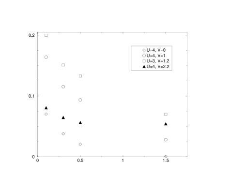
Figure 10: Relative errors of the RVA results compared to the DMRG ones. The unfilled symbols are for calculations where $U>2V$; these choices give a BOW ground state. On the contrary, the filled triangles correspond to calculations where $U<2V$; then a CDW ground state is stabilized.

4 Conclusions and Perspectives

To conclude, we have presented in this note the Recurrent Variational Approach and, more specifically, its first application to the electronic structure of conjugated polymers. The ansatz built here (26), shows some nice similarities with the trial state (3) made for the two–leg ladder.

By comparisons with Density Matrix Renormalization Group calculations, we think this trial wave function encouraging and a good starting point for further improvements. Moreover, we believe such kind of simple wave functions useful to get some analytical insight into physical phenomena [Pleutin and Fave (1998), Pleutin (1999)].

Two natural extensions of this work are currently in progress: first, it is possible, in some extents, to improve the simple ansatz (26) by including more local configurations; second, it is also possible to apply the method to other conjugated polymers of current interests as the poly–paraphenylene and the poly–paraphenylenevinylene.

References

- Anderson (1987) P.W. Anderson Science 235, 1196, 1987
- Baeriswyl (1992) D. Baeriswyl, D.K. Campbell and S. Mazumdar, in Conjugated Conducting Polymers, edited by H. Kiess (Springer-Verlag, Heidelberg, 1992), pp7-133.
- Barnes (1993) T. Barnes, E. Dagotto, J. Riera and E. S. Swanson, Phys. Rev. B 47, 3196 (1993)
- Bendazzoli (1999) G.L. Bendazzoli, S. Evangelisti, G. Fano, F. Ortolani and L. Ziosi, J. Chem. Phys. 110, 1277 (1999)
- Bethe (1931) H. Bethe, Z Physik 71, 205 (1931)
- Boman and Bursill (1998) M. Boman and R.J. Bursill, Phys. Rev. B57, 15167 (1998)
- Chandross (1999) M. Chandross, Y. Shimoi and S. Mazumdar, Phys. Rev. B 59, 4822 (1999).
- Cizek and Paldus (1971) J. Cizek and J. Paldus, J. Intern. J. Quantum Chem. 5, 359 (1971)
- Dagotto and Rice (1996) E. Dagotto and T.M. Rice, Science 271, 619 (1996)
- Dukelsky (1998) J. Dukelsky, M.A. Martín-Delgado, T. Nishino and G. Sierra, Europhysics Lett. 43, 457 (1998)
- Eder (1999) R. Eder, Phys. Rev. B59, 13810 (1999)
- Gopalan (1994) S. Gopalan, T.M. Rice and M. Sigrist, Phys. Rev. B49, 8901 (1994)
- Haldane (1981) F.D.M. Haldane, J. Phys. C 14, 2585 (1981)
- Heeger (1988) A.J. Heeger, S. Kivelson, J.R. Schrieffer and W.P. Su, Rev. Mod. Phys. 60, 781 (1988)
- Hückel (1931) E. Hückel, Z. Phys. 70, 204 (1931)
- Jeckelmann (1998) E. Jeckelmann, Phys. Rev. B57, 11838 (1998).
- Kim (1999) E.H. Kim, G. Sierra and D. Duffy, cond-mat/9902107
- Mazumdar and Campbell (1985) S. Mazumdar and D.K. Campbell, Phys. Rev. Lett. 55, 2067 (1985)
- Mukhopadhyay (1995) D. Mukhopadhyay, G.W. Hayden and Z.G. Soos, Phys. Rev. B51, 9476 (1995).
- Ovchinnikov (1973) A.A. Ovchinnikov, I.I. Ukrainskii and G.V. Kventsel, Sov. Phys.-Usp. 15, 575 (1973)
- Pariser and Parr (1953) R. Pariser and R.G. Parr, J. Chem. Phys. 21, 767 (1953)
- Pauling (1960) L. Pauling, The nature of the chemical bond, Cornell University press (1960)
- Peschel (1999) Density-Matrix Renormalization - A New Numerical Method in Physics, Lecture Notes in Physics, eds I. Peschel, X. Wang, M. Kaulke, and K. Hallberg, Springer-Verlag, 1999.
- Pleutin and Fave (1998) S. Pleutin and J.L. Fave, J. of Phys. : Condens. Matter 10, 3941 (1998)
- Pleutin (1999) S. Pleutin, in preparation, (1999)
- Pople (1953) J.A. Pople, Trans. Faraday Soc. 49, 1375 (1953)
- Pople and Walmsley (1962) J.A. Pople and S.H. Walmsley, Mol. Phys. 5, 15 (1962)
- Ramasesha (1996) S. Ramasesha, S.K. Pati, H.R. Krishnamurthy, Z. Shuai and J.L. Bredas, Phys. Rev. B54, 7598 (1996)
- Rice (1979) M.J. Rice, Phys. Lett. 71A, 152 (1979)
- Roncaglia (1999) M. Roncaglia, G. Sierra and M.A. Martín-Delgado, cond-mat/9904286
- Salem (1966) L. Salem, Molecular Orbital Theory of Conjugated Systems (Benjamin, London 1966).
- Sariciftci (1997) Primary photoexcitations in Conjugated Polymers: Molecular Exciton versus Semiconductor Band Model, edited by N.S. Sariciftci (World Scientific Publishing, Singapore, 1997).
- Shuai (1998) Z. Shuai, J.L. Bredas, A. Saxena and A.R. Bishop, J. Chem. Phys. 109, 2549 (1998)
- Sierra and Martín-Delgado (1997) G. Sierra and M.A. Martín-Delgado, Phys. Rev. B 56, 8774 (1997)
- Sierra (1998) G. Sierra, M.A. Martín-Delgado, J. Dukelsky, S. R. White and D. J. Scalapino, Phys. Rev.B 57, 11666 (1998)
- Sierra (1999) G. Sierra, M.A. Martín-Delgado, S.R. White, D.J. Scalapino, J. Dukelsky, Phys. Rev. B59, 7976 (1999)
- Simpson (1955) W.T. Simpson, J. Am. Chem. Soc. 77, 6164 (1955).
- Soos (1997) Z.G. Soos, M.H. Hennessy and D. Mukhopadhyay, in Primary photoexcitations in Conjugated Polymers: Molecular Exciton versus Semiconductor Band Model, edited by N.S. Sariciftci (World Scientific Publishing, Singapore, 1997).
- Su (1979) W.P. Su, J.R. Schrieffer and A.J. Heeger, Phys. Rev. Lett. 42, 1698 (1979)
- Tavan and Schulten (1987) P. Tavan and K. Schulten, Phys. Rev. B36, 4337 (1987)
- White (1993) S.R. White, Phys. Rev. B48, 10345 (1993).
- White and Huse (1993) S.R. White and D.A. Huse Phys. Rev. B 48, 3844 (1993)