Semiclassical mechanics of a non-integrable spin cluster

Abstract

We study detailed classical-quantum correspondence for a cluster system of three spins with single-axis anisotropic exchange coupling. With autoregressive spectral estimation, we find oscillating terms in the quantum density of states caused by classical periodic orbits: in the slowly varying part of the density of states we see signs of nontrivial topology changes happening to the energy surface as the energy is varied. Also, we can explain the hierarchy of quantum energy levels near the ferromagnetic and antiferromagnetic states with EKB quantization to explain large structures and tunneling to explain small structures.

I Introduction

When $S$ is large, spin systems can be modeled by classical and semiclassical techniques. Here we reserve “semiclassical” to mean not only that the technique works in the limit of large $S$ (as the term is sometimes used) but that it implements the quantum-classical correspondence (relating classical trajectories to quantum-mechanical behavior).

Spin systems (in particular $S=1/2$) are often thought as the antithesis of the classical limit. Notwithstanding that, classical-quantum correspondence has been studied at large values of $S$ in systems such as an autonomous single spin [3], kicked single spin [4], and autonomous two [5] and three [6] spin systems.

When the classical motion has a chaotic regime, for example, the dependence of level statistics on the regularity of classical motion has been studied [5, 6]. In regimes where the motion is predominantly regular, the pattern of quantum levels of a spin cluster can be understood with a combination of EBK (Einstein-Brillouin-Keller, also called Bohr-Sommerfeld) quantization and tunnel splitting (Sec. V is a such a study for the current system.) The latter sort of calculation has potential applications to some problems of current numerical or experimental interest. Numerical diagonalizations for extended spin systems (in ordered phases) on lattices of modest size ($10$ to $36$ spins) may be analyzed by treating the net spin of each sublattice as a single large spin and thereby reducing the system to an autonomous cluster of a few spins; the clustering of low-lying eigenvalues can probe symmetry breakings that are obscured in a system of such size if only ground-state correlations are examined. [7] Nonlinear self-localized modes in spin lattices [8], which typically span several sites, have to date been modeled classically, but seem well suited to semiclassical techniques. Another topic of recent experiments is the molecular magnets [9] such as $\rm Mn_{12}Ac$ and $\rm Fe_{8}$, which are more precisely modeled as clusters of several interacting spins rather than a single large spin; semiclassical analysis may provide an alternative to exact diagonalization techniques [10] for theoretical studies of such models.

In this paper, we will study three aspects of the classical-correspondence of an autonomous cluster of three spins coupled by easy-plane exchange anisotropy, with the Hamiltonian

$${H}=\left[\sum_{i=1}^{3}{\mathbf{S}}_{i}\cdot{\mathbf{S}}_{i+1}-\sigma{\mathbf{S}}_{i}^{z}{\mathbf{S}}_{i+1}^{z}\right],$$ (1)

This model was introduced in Ref. [11], a study of level repulsion in regions of $(E,\sigma)$ space where the classical dynamics is predominantly chaotic [6]. Eq. (1) has only two nontrivial degrees of freedom, since it conserves total angular momentum around the z-axis. As did Ref. [11] we consider only the case of $\sum_{i}{\mathbf{S}}_{i}^{z}=0.$ While studying classical mechanics we set $|{\mathbf{S}}|=1;$ to compare quantum energy levels at different $S$, we we divide energies by by $S(S+1)$ to normalize them. The classical maximum energy, $E=3$, occurs at the ferromagnetic (FM) state – all three spins are coaligned in the equatorial (easy) plane. The classical ground state energy is $E=-1.5$, in the antiferromagnetic (AFM) state, in which the spins lie $120^{\circ}$ apart in the easy plane; there are two such states, differing by a reflection of the spins in a plane containing the $z$ axis. Both the FM and AFM states, as well as all other states of the system, are continuously degenerate with respect to rotations around the $z$-axis. The classical dynamics follows from the fact that $\cos\theta_{i}$ and $\phi_{i}$, are conjugate, where $\theta_{i}$ and $\phi_{i}$ are the polar angles of the unit vector ${\mathbf{S}}_{i}$; then Hamilton’s equations of motion say

$$d\cos\theta_{i}/dt = \hbar^{-1}\partial{H}/\partial\phi_{i};$$ (2)

$$d\phi_{i}/dt = -\hbar^{-1}\partial{H}/\partial\phi_{i}.$$ (3)

In the rest of this paper, we will first introduce the classical dynamics by surveying the fundamental periodic orbits of the three-spin cluster, determined by numerical integration of the equations of motion (Sec II). The heart of the paper is Sec. III: starting from the quantum density of states (DOS) obtained from numerical diagonalization, we apply nonlinear spectral analysis to detect the oscillations in the quantum DOS caused by classical periodic orbits; to our knowledge, this is the first time the DOS has been related to specific orbits in a multi-spin system. Also, in Sec. IV we smooth the DOS and compare it to a lowest-order Thomas-Fermi approximation counted by Monte Carlo integration of the classical energy surface; a flat interval is visible in the quantum DOS between two critical energies where the topology of the classical energy surface changes. Finally, in Sec. V, we use a combination of EBK quantization and tunneling analysis to explain the clustering patterns of the quantum levels in our system.

II Classical periodic orbits

Our subsequent semiclassical analysis will depend on identification of all the fundamental orbits and their qualitative changes as parameters are varied. Examining Poincaré sections and searching along symmetry lines of the system, we found four families of fundamental periodic orbits for the three-spin cluster. Figure 1 is an illustration of their motion, and Figure 2 gives classical energy-time curves. Orbits of types (a)-(c) are always at least threefold degenerate, since one spin is different from the other two; orbits of types (a)-(c) are also time-reversal invariant. Orbit (a), the counterbalanced orbit, exists when $E>-1$ (including the FM limit) and, in the range $0<\sigma<1$ which we’ve studied, is always stable. Orbit (b), the unbalanced orbit, is unstable and exists when $E<E_{p},$ where

$$E_{p}={3\over 4}\sigma-{3\over 2}.$$ (4)

Orbits of type (c), or stationary spin exist at all energies. Type (c) orbits are are unstable in the range, $-1>E>3.$ Below $E=-1$ the stationary spin orbit bifurcates into two branches without breaking the symmetry of the ferromagnetic ground state. At

$$E_{c}(\sigma)={3-3\sigma+\sigma^{2}\over\sigma-2},$$ (5)

one branch vanishes and the other branch bifurcates into two orbits that are distorted spin waves of the two AFM ground states. (Below, in Sections IV and V, we will discuss topology changes of the entire energy surface.) Although they are not related by symmetry, all orbits of type (c) at a particular energy have the same period.

Orbits of type (d), or three-phase orbits are named in analogy to three-phase AC electricity, as spin vectors move along distorted circles, $120^{\circ}$ out of phase. The type (d) orbits break time-reversal symmetry and are hence at least twofold degenerate. A symmetry-breaking pitchfork bifurcation of the (d) family occurs (for $\sigma=0.5$ around $E=-0.75$) at which a single stable orbit, approaching from high energy, bifurcates into an unstable and two stable precessing three-phase orbits without period doubling. [12] (Strictly speaking, the precessing three-phase orbits are not periodic orbits of the three-spin system, since after one “period” the spin configuration is not the same as before, but rather, all three spins are rotated by the same angle around the $z$-axis). The unstable three-phase orbit disappears quickly as we lower energy, but the precessing three-phase orbits persist until $E=-1.5,$ and become intermittently stable and unstable in a heavily chaotic regime near $E_{A},$ but regain stability before $E\rightarrow-1.5$: thus in the AFM limit, orbits (c) are stable while orbits (b) are unstable. [16] More information on the classical mechanics of this system appears in Refs. [13] and [14].

III Orbit spectrum analysis

Gutzwiller’s trace formula, the central result of periodic orbit theory, [15]

$$\rho(E)={\mathrm{Re}}\sum_{p}A_{p}(E)\exp[iS_{p}(E)/\hbar]+\rho_{tf}(E),$$ (6)

decomposes the quantum DOS $\rho(E)$ into a sum of oscillating terms contributed by classical orbits indexed by $p,$ where $S_{p}(E)$ is the classical action, and $A_{p}(E)$ is a slowly varying function of the period, stability and geometric [17] properties of the orbit $p$), plus the zeroth-order Thomas-Fermi term,

$$\rho_{tf}(E)=\int{d^{2N}{\tilde{z}}\over(2\pi\hbar)^{N}}\delta\left(E-H({\tilde{z}})\right),$$ (7)

This integral over phase space ${\tilde{z}}$ is simply proportional to the area of the energy surface. We do not know of any mathematical derivation of (6) in the case of a spin system.

At a fixed H, the orbit spectrum is, as function of $\tau,$ the power spectrum of $\rho(E)$ inside the energy window, $H-\Delta H/2<E<H+\Delta H/2.$ (Figure 3, explained below, is an example of an orbit spectrum.) Since the classical period $\tau_{p}(E)=\partial S_{p}(E)/\partial E,$ Eq. (6) implies that $O(H,\tau)$ is large if there exists a periodic orbit with energy $H$ and period $\tau.$ The orbit spectrum can be estimated by Fourier transform, [18]

$$O(H,\tau)=\left|\int_{H-\Delta H/2}^{H+\Delta H/2}\rho(E)e^{-i\hbar^{-1}E\tau}dE\right|^{2}.$$ (8)

Variants of Eq. (8) have been used to extract information about classical periodic orbits from quantum spectra. [19, 20] Unfortunately, the resolution of the Fourier transform is limited by the uncertainty principle, $\delta E\delta t=\hbar/2.$

Nonlinear spectral estimation techniques, however, can surpass the resolution of the Fourier transform. [21] One such technique, harmonic inversion, has been successfully applied to scaling systems [22] – i.e., systems like billiards or Kepler systems in which the (classical and quantum) dynamics at one energy are identical to those at any other energy, after a rescaling of time and coordinate scales. In a scaling system, windowing is unnecessary because there are no bifurcations and the scaled periods of orbits are constant. In this section, we will apply nonlinear spectral estimation to our system (1), which is nonscaling. [23]

A Diagonalization

To get the quantum level spectrum, we wrote software to diagonalize arbitrary spin Hamiltonians polynomial in (${\mathbf{S}}_{i}^{x},{\mathbf{S}}_{i}^{y},{\mathbf{S}}_{i}^{z}$), where $i$ is an index running over arbitrary $N$ spins of arbitrary (and often large) spin $S$. The program, written in Java, takes advantage of discrete translational and parity symmetries by constructing a basis set in which the Hamiltonian is block diagonal, letting us diagonalize the blocks independently with an optimized version of LAPACK. Picturing the spins in a ring, the Hamiltonian Eq. (1) is invariant to cyclic permutations of the spins, so the eigenstates are states of definite wavenumber [6] $k=0,\pm{2\pi\over 3}$ (matrix blocks for $k=\pm{2\pi\over 3}$ are identical by symmetry). In the largest system we diagonalized (three-spin cluster with $S=65$) , the largest blocks contained $N=4620$ states.

B Autoregressive approach to construct spectrum

The input to an orbit spectrum calculation is the list of discrete eigenenergies with total $S_{z}=0$; no other information on the eigenstates (e.g. the wavenumber quantum number) is necessary. This level spectrum is smoothed by convolving with a Gaussian (width $10^{-3}$ for Figure 3) and discretely sampling over energy (with sample spacing $\delta=4.5\times 10^{-4}$.)

We estimate the power spectrum by the autoregressive (AR) method. AR models a discretely sampled input signal, $y_{i}$ (in our case the density of states) with a process that attempts to predict $y_{i}$ from its previous values,

$$y_{i}=\sum_{j=1}^{N}a_{i}y_{i-j}+x_{i}.$$ (9)

Here $N$ is a free parameter which determines how many spectral peaks that model can fit; Refs. [21] and [24] discuss guidelines for choosing $N$. Fast algorithms exist to implement least-squares, i.e. to choose $N$ coefficients $a_{i}$ to minimize (within constraints) $\sum x_{i}^{2}$; of these we used the Burg algorithm [21].

To estimate the power spectrum, we discard the original $x_{i}$ and model $x_{i}$ with uncorrelated white noise. Thinking of Eq. (9) as a filter acting on $x_{i},$ the power spectrum of $y_{i}$ is computed from the transfer function of Eq. (9) and is

$$P(\nu)={<x_{i}^{2}>\over 1-\sum_{j=1}^{N}a_{j}e^{i\nu\delta}}.$$ (10)

Unlike the discrete Fourier transform, $P(\nu)$ can be evaluated at any value of $\nu.$ In our application, of course, $\delta$ has units of energy, so $\nu$ (more exactly $\nu/\hbar$) actually has units of time and is to be identified with $\tau$ in (8).

C Orbit spectrum results and discussion

Figure 3 shows the orbit spectrum of our system with $S=65$ and $\sigma=0.5.$; it is displayed as a $500\times 390$ array of pixels, colored light where $O(H,\tau)$ is large. Each horizontal row is the power spectrum in an energy window centered at $H;$ we stack rows of varying $H$ vertically. With a window width 250 energy samples long ($\delta H=0.1125,$) we fit $N=150$ coefficients in Eq. (9). To improve visual resolution, we let windows overlap and spaced the centers of successive windows 25 samples apart.

Comparing Figure 3 and Figure 2 we see that our orbit spectrum detects the fundamental periodic orbits as well as multiple transversals of the orbits. Interestingly, we produced Figure 3 before we had identified most of the fundamental orbits; Figure 3 correctly predicted three out of four families of orbits.

We believe that, given the same data, the AR method normally produces a far sharper spectrum. This is not surprising, since the Fourier analysis allows the possibility of orbit-spectrum density at all $\tau$ values, whereas AR takes advantage of our a priori knowledge that there are only a few fundamental periodic orbits and hence only a few peaks. We have compared the Fourier and AR versions of the spectrum in a few cases, but have not systematically tested them against each other.

Unfortunately, the artifacts and limitations of the AR method are less understood than those of the Fourier transform. At high energies, the classical periods are nearly degenerate, so we expect closely spaced spectral peaks in the orbit spectrum. In this situation, the Burg algorithm vacillates between fitting one or two peaks causing the braiding between the (a) and (c) orbits (labeled in Figure 2) in Figure 3. Also, in the range $-1<E<-1.3,$ where classical chaos is widespread, bifurcations increase the number of contributing orbits so that we cannot interpret the orbit spectrum for $\tau>10.$

IV Averaged density of states

The lowest-order Thomas Fermi approximation, Eq. (7) predicts that the area of the classical energy surface is proportional to the DOS. We verify this in Figure 4, a comparison of the heavily smoothed quantum DOS to the area of the energy surface computed by Monte Carlo integration.

An energy interval is visible in which the quantum DOS appears to be constant; we then verified that the classical DOS (which is more precise) is constant to our numerical precision; a similar interval was observed for all values of $\sigma$. We identified this interval as $(E_{p},-1)$, where the endpoints are associated with changes in the topology of the energy surface as the energy varies.

At energies below $E_{c}$ (see Eq. (5)), the energy surface consists of two disconnected pieces, one surrounding each AFM ground state. The two parts coalesce as the energy surface becomes multiply connected at $E_{c}.$ For $E<E_{p},$ (see Eq. (4)) the anisotropic interaction confines the spins to a limited band of latitude away from the poles. At $E_{p}$ it becomes possible for spins to pass over the poles. At $E=-1,$ the holes that appeared in the energy surface at $E_{c}$ close up. A discontinuity in the slope of the area of the energy surface occurs at energy $E_{c}$ (not visible in Figure 4); in the range $E_{p}<E<-1$ the area of the energy surface (and hence the slowly varying part of the DOS) seems to be constant as a function of energy.

In the special isotropic ($\sigma=0$) case, the flat interval is $(-1.5,-1)$ and it can be analytically derived that the DOS is constant there. This is simplest for the smoothed quantum DOS, since for $n=1,2,\ldots$ there are clusters of $n$ energy levels with level spacing proportional to $n$. (A derivation also exists for the classical case, but is less direct.) We have no analytic results for general $\sigma$.

This flat interval is specific to our three-spin cluster, but we expect that the compactness of spin phase space will, generally, cause changes in the energy surface topology of spin systems that do not occur in traditionally studied particle systems.

V Level clustering

The quantum levels with total ${\mathbf{S}}_{z}=0$ show rich patterns of clustering, some of which are visible on Figure 5. The levels that form clusters correspond to three different regimes of the classical dynamics in which the motion becomes nearly regular: (1) the FM limit (not visible in Figure 5; (2) the AFM limit (bottom edge of Figure 5) and (3) the isotropic limit $\sigma=0$ (left edge of Figure 5). Indeed, the levels form a hierarchy in as the clusters break up into subclusters. In this section, we first approximately map the phase space from four coordinates to two coordinates – with the topology of a sphere. (Two of the original six coordinates are trivial, or decoupled, due to symmetry, as noted in Sec. II. Then, using Einstein-Brillouin-Kramers (EBK) quantization some consideration of quantum tunneling, many features of the level hierarchy will be understood.

A Generic behavior: the polyad phase sphere

In all three limiting regimes, the classical dynamics becomes trivial. For small deviations from the limit, the equations of motion can be linearized and one finds that the trajectory decomposes into a linear combination of two harmonic oscillators with degenerate frequency $\omega$, i.e., in a 1:1 resonance; the oscillators are coupled only by higher-order (=nonlinear) terms.

There is a general prescription for understanding the classical dynamics in this situation [25]. Near the limit, the low-excited levels have approximate quantum numbers $n_{1,2}$ such that the excitation energy $\Delta E_{i}$ in oscillator $i$ is $\hbar\omega(n_{i}+1/2)$. (In the FM limit, regime (1), this difference is actually measured downwards from the energy maximum.) Clearly, the levels with a given total quantum number $P\equiv(n_{1}+n_{2}+1)$ must have nearly degenerate energies, and thus form a cluster of levels, which are split only by the effects (to be considered shortly) of the anharmonic perturbation. A level cluster arising in this fashion is called a polyad [25].

To reduce the classical dynamics, make a canonical transformation to the variables $\Phi$ and ${\bf P}\equiv(P_{x},P_{y},P_{z})$, where $\Phi$ is the mean of the oscillators’ phases and $\Psi_{x}$ is their phase difference, and

$$P_{x} \equiv {1\over 2}(n_{1}-n_{2}),$$ (11)

$$(P_{y},P_{z}) \equiv 2\sqrt{(n_{1}+1/2)(n_{2}+1/2)}(\cos\Psi_{x},\sin\Psi_{x}),$$ (12)

Here $\Phi$ is the fast coordinate, with trivial dynamics $d\Phi/dt=\omega$ in the harmonic limit. The slow coordinates $\bf P$ follow a trajectory confined to the “polyad phase sphere” $|{\bf P}|=P$, since $\Delta E=\hbar\omega P$ is conserved by the harmonic-order dynamics. The reduced dynamics on this sphere is properly a map ${\bf P}_{i}\to{\bf P}_{i+1}$, defined by (say) the Poincaré section at $\Psi_{x}=0({\rm mod}\;2\pi)$. But $d{\bf P}/dt$ contains only higher powers of the components of $\bf P$, so near the harmonic (small $P$) limit, $|{\bf P}_{i+1}-{\bf P}_{i}|$ vanishes and the reduced dynamics becomes a flow.  [26] At the limit in which it is a flow, an effective Hamiltonian $I$ can be defined so that the dynamics becomes integrable. [27] Applying EBK quantization to the reduced dynamics on the polyad phase sphere gives the splitting of levels within a polyad cluster. (Near the harmonic limit, the energy scale of $I$ is small compared to the splitting between polyads.)

In all three of our regimes, we believe this flow has the topology shown schematically in Figure 6. [28] Besides reflection symmetry about the “equator”, it also has a threefold rotation symmetry around the $P_{z}$ axis, which corresponds to the cyclic permutation of the three spins. [29] (Figure 6 is natural for the three-spin system because it is the simplest generic topology of the phase sphere with that threefold symmetry.) The reduced dynamics has two symmetry-related fixed points at the “poles” $P_{z}=\pm P$, which always correspond to motions of the three-phase sort like (d) on Figure 1. There are also three stable and three unstable fixed points around the “equator”.

The KAM tori of the full dynamics correspond to orbits of the reduced dynamics. These orbits follow contours of the effective Hamiltonian $I$ of the reduced dynamics (as in Figure 6). In view of the symmetries mentioned,

$$I=\alpha P_{z}^{2}+\beta(P_{x}^{3}-3P_{x}P_{y}^{2})+{\rm const}$$ (13)

to leading order, where $\alpha$,$\beta$, and the constant may depend on $\sigma$, $S$, and $P$.

The KAM tori surrounding the three-phase orbits represented by the “poles” are twofold degenerate, while the tori in the stable resonant islands represented on the “equator” are threefold degenerate. Hence, the EBK construction produces degenerate subclusters containing two or three levels depending on the energy range within the polyad cluster.

The fraction of levels in one or the other kind of subcluster is proportional to the spherical areas on the corresponding side of the separatrix, which passes through the unstable points in Figure 6. These areas in turn depend on the ratio of the first to the second term in Eq. (13), i.e. $\alpha P^{2}/\beta P^{3}$. Evidently, as one moves away from the harmonic limit to higher values of $P$, one universally expects to have a larger and larger fraction of threefold subclusters.

Given the numerical values of energy levels in a polyad, we can estimate the terms of Eq. (13) in the following fashion: (i) the energy difference between the highest and lowest 3-fold subcluster is the difference between the stable and unstable orbits on the equator, which is $2\beta P^{3}$ according to (13); (ii) the mean of the highest and lowest 3-fold subcluster would be the energy all around the equator if $\beta$ were to vanish; the difference between this energy and that of the farthest 2-fold subcluster in the polyad is $\alpha P^{2}$ according to (13).

Furthermore, tunneling between nearby tori creates fine structure splitting inside the sub-clusters. The slow part of the dynamics on the polyad phase sphere, is identical to that of a single semiclassical spin with (13) as its effective Hamiltonian, so the effective Lagrangian is essentially the same, too. Then different tunneling paths connecting the same two quantized orbits must differ in phase by a topological term, with a familiar form proportional to the (real part of the) spherical area between the two paths. [30]

B Results

Here we summarize some observations made by examination of polyads in the three regimes, for a few combinations of $S$ and $\sigma$.

1 Ferromagnetic limit

This regime is the best-behaved in that regular behavior persists for a wide range of energies. The ferromagnetic state, an energy maximum, is a fixed point of the dynamics; around it are “spin-wave” excitations (viewing our system as the 3-site case of a one dimensional ferromagnet). These are the two oscillators from which the polyad is constructed. Thus, the “pole” points in Figure 6 correspond to “spin waves” propagating clockwise or counterclockwise around the ring of three spins, an example of the “three-phase” type of orbit. The stable and unstable points on the “equator” are identified respectively with the orbits (a) and (c) of Figure 1. Classically, in this regime, the three-phase orbit is the fundamental orbit with lowest frequency $\omega_{3-phase}$; thus the corresponding levels in successive polyads have a somewhat smaller spacing $\hbar\omega_{3-phase}$ than other levels, and they end up at the top of each polyad. (Remember excitation energy is measured downwards from the FM limit.) Indeed, we observe that the high-energy end of each polyad consists of twofold subclusters and the low-energy end consists of threefold subclusters.

We see a pattern of fine structure (presumably tunnel splittings) which is just like the pattern in the four-spin problem.[7, 31] Namely, throughout each polyad the degeneracies of successive levels follow the pattern (2,1,1,2) and repeat. (Here – as also for regime 3 – every “2” level has $k=\pm 1$ and every “1” level has $k=0$, where wavenumber $k$ was defined in Sec. III A.) Numerical data show that (independent of $S$) the pattern (starting from the lowest energy) begins (2112…) for even $P$, but for odd $P$ it begins (1221…).

In the energy range of twofold subclusters, the levels are grouped as (2)(11)(2), i.e. one tunnel-split subcluster between two unsplit subclusters(and repeat); in the threefold subcluster regime, the grouping is (21)(12), so that each subcluster gets tunnel-split into a pair and a single level, but the sense of the splitting alternates from one subcluster to the next.

An analysis of $\sigma=0.4$, $S=30$ showed that the fraction of threefold subclusters indeed grows from around 0.3 for small $P$ to nearly $0.5$ at $P\approx 40$. Furthermore, when $\alpha P^{2}$ and $\beta P^{3}$ were estimated by the method described near the end of Subsec. V A, they indeed scaled as $P^{2}$ and $P^{3}$ respectively.

2 Antiferromagnetic limit

This regime occurs at $E<E_{c}(\sigma)$, where $E_{c}(\sigma)$ is given by (5). That means the classical energy surface is divided into two disconnected pieces, related by a mirror reflection of all three spins in any plane normal to the easy plane. Analogous to regime one, two degenerate antiferromagnetic “spin waves” exist around either energy minimum, and the polyad states are built from the levels of these two oscillators. Thus the clustering hierarchy outlined in Sec. V A – polyads clusters, EBK-quantization of $I$, and tunneling over barriers of $I$ on the polyad phase sphere – is repeated within each disconnected piece, leading to a prediction that all levels should be twofold degenerate.

Consequently, on the level diagram (Figure 5), there should be half the apparent level density below the line $E=E_{c}(\sigma)$ as above it. Indeed, a striking qualitative change in the apparent level crossing behavior is visible at that line (shown dashed in the figure).

Actually, tunneling is possible between the disconnected pieces of the energy surface and may split these degenerate pairs. In fact this hyperfine splitting happens to 1/3 of the pairs, again following the (2112) pattern within a given polyad. This (2112) pattern starts to break up as the energy moves away from the AFM limit; even for large $S$ ($30$ or $65$), this breakup happens already around the polyad with $P=10$, so it is much harder than in the FM case to ascertain the asymptotic pattern of subclustering. We conjecture that the breakup may happen near the energies where, classically, the stable periodic orbits bifurcate and a small bit of phase space goes chaotic.

The barrier for tunneling between the disconnected energy surfaces has the energy scale of the bare Hamiltonian, which is much larger (at least, for small $P$) than the scale of effective Hamiltonian $I$ which provides the barrier for tunneling among the states in a subcluster. Hence, the hyperfine splittings are tiny compared to the fine splittings discussed at the end of Subsection V A. To analyze numerical results, we replace a degenerate level pair by one level and a hyperfine-split pair by the mean level, and treat the result as the levels from one of the two disconnected polyad phase spheres, neglecting tunneling to the other one.

Then in the AFM limit, the “pole” points in Figure 6 again correspond to spin waves propagating around the ring, while the stable and unstable points on the equator are (c) and (b) on Figure 1. The three-phase orbit is the highest frequency orbit in the AFM limit, [14] so again the twofold and threefold subclusters should occur at the high and low energy ends of each polyad cluster. What we observe, however, is that all the subclusters are twofold, except the lowest one is often threefold.

3 Isotropic limit

This regime will includes only $S_{\rm tot}\leq S$ i.e. $E<-1$ – the same regime in which the flat DOS was observed (Sec. IV). Above the critical value $E=-1$, the levels behave as in the “FM limit” described above.

At $\sigma=0$, it is well-known that the quantum Hamiltonian reduces to ${\scriptstyle{1\over 2}}[S_{\rm tot}^{2}-3S(S+1)]$. Thus each level has degeneracy $P\equiv 2S_{\rm tot}+1$. (That is the number of ways three spins $S$ may be added to make total spin $S_{\rm tot}$, and each such multiplet has one state with $S^{z}_{\rm tot}=0$.) When $\sigma$ is small, these levels split and will be called a polyad. [32]

Classically, at $\sigma=0$ the spins simply precess rigidly around the total spin vector. These are harmonic motions of four coordinates; hence the polyad phase sphere can be constructed by (12). From the threefold symmetry, there should again be three orbit types as represented generically by Figure 6 and Eq. (13). For example, an umbrella-like configuration in which the three spin directions are equally tilted out of their plane corresponds to a three-phase type orbit, with two cases depending on the handedness of the arrangement. A configuration where one spin is parallel/antiparallel to the net moment, and the other two spins offset symmetrically from it), follows one of the threefold degenerate orbits.

Numerically, the level behavior in the near-isotropic limit is similar to the near-FM limit. The fine structure degeneracies are a repeat of the (2112) pattern as in the other regimes; the lowest levels of any polyad always begin with (1221). The fraction of threefold subclusters is large here and, as expected, grows with $S$, (from 0.5 to 0.7 in the case $S=15$). However, the energy scales of $\alpha P^{2}$ and $\beta P^{3}$ behave numerically as $\sigma P^{0}$ and $\sigma P^{1}$. What is different about the isotropic limit is that the precession frequency – hence the oscillator frequency $\omega$ – is not a constant, but is proportional to $S_{\rm tot}$. Since perturbation techniques [27] give formulas for $I$ with inverse powers of $\omega$, it is plausible that $\alpha$ and $\beta$ in (13) include factors of $P^{-2}$ here, which were absent in the other two regimes.

VI Conclusion and summary

To summarize, by using detailed knowledge of the classical mechanics of a three spin cluster [14], we have studied the semiclassical limit of spin in three ways. First, using autoregressive spectral analysis, we identified the oscillating contributions that the fundamental orbits of the cluster make to the density of states, in fact, we detected the quantum signature of the orbits before discovering them. Secondly, we verified that the quantum DOS is proportional to the area of the energy surface; we also observed kinks in the smoothed quantum DOS, which are the quantum manifestation of topology changes of the classical energy surface; such topology changes, we expect, are more common in spin systems than particle phase space, since even a single spin has a nontrivial topology. Finally, we have identified three regimes of near-regular behavior in which the levels are clustered according to a four-level hierarchy, and we explained many features qualitatively in terms of a reduced, one degree-of-freedom system. This system appears promising for two extensions analgous to Ref. [7]: tunnel amplitudes (and their topological phases) could be computed more explicitly; also, the low-energy levels from exact diagonalization of a finite piece of the anisotropic-exchange antiferromagnet on the triangular lattice could probably be mapped to three large spins and analyzed in the fashion sketched above in Sec. V.

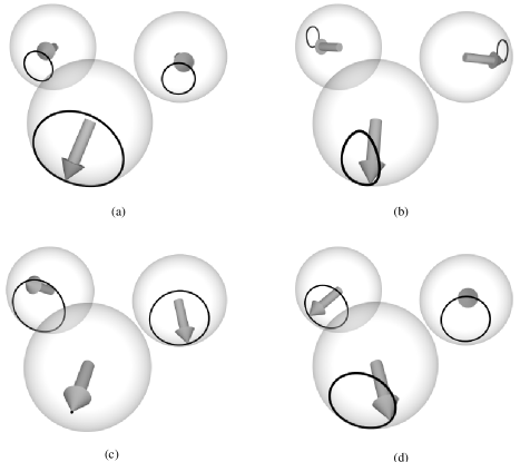
FIG. 1.: Fundamental periodic orbits of the three-spin cluster. (a) Counterbalanced, (b) unbalanced orbits, (c) stationary spin, and (d) three-phase.

FIG. 2.: Energy-period curve of the three spin system with $\sigma=0.5$. The curves (a), (b), (c) and (d) are four families of periodic orbits . Below the obvious bifurcation around $E=-0.75$, orbit (d) is not literally a periodic orbit of the three spins, but only in a reduced two degree of freedom system (wherein one identifies states related by a rotation of all three spins about the $z$ axis.

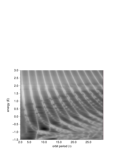
FIG. 3.: Orbit spectrum for $S=65,\sigma=0.5.$ The horizontal axis is classical period, and the vertical axis is energy. Peaks of the orbit spectrum are white and valleys are black.

FIG. 4.: The density of states of a $S=40$ three spin cluster with $\sigma=0.1,$ smoothed with a Gaussian $\exp[-({E/\delta})^{2}]$ with $\delta=0.01.$ The Thomas-Fermi density of states is very flat in the range $E_{p}<E<-1,$ with $E_{p}=-1.43.$

FIG. 5.: Energy levels as a function of $\sigma$ for an $S=10$ three spin cluster. The dashed line is the coalescence energy $E_{c}(\sigma)$ defined by equation Eq. (5).

FIG. 6.: Topology of orbits for a generic phase sphere with 3-fold symmetry. The phase space is decomposed into one “fast” action variable, which is transverse to the 3-space of the sphere, and three “slow” variables; of these, the energy is a function of radius and is conserved. Contours are shown of an effective Hamiltonian $I$, with the direction of “slow” motion indicated by arrows. Tunneling takes place between symmetry-related orbits across the saddle points of $I$, as indicated by the dashed lines. The stationary points of this two-dimensional flow labeled (b), (c), and (d) correspond near the antiferromagnetic ground state to the periodic orbits of the full system labeled the same way in Figure 1; the labeling would differ somewhat for the near-ferromagnetic or near-isotropic regimes (see Sec. V B).

- [1] Current address: Max-Planck-Institute for the Physics of Complex Systems, 38 Nöthnitzer Str., Dresden, D-01187 Germany
- [2] Author to whom correspondence should be addressed.
- [3] R. Shankar, Phys. Rev. Lett. 45, 1088 (1980).
- [4] F. Haake, M. Kus, and R. Scharf, Z. Phys. B 65, 381 (1987). The classical-quantum correspondence has been studied extensively in this system, but the Hamiltonian is time-varying and unlike that of interacting spins,
- [5] N. Srivastava and G. Müller, Z. Phys. B 81, 137 (1990).
- [6] K. Nakamura, Quantum Chaos: A new paradigm of nonlinear dynamics, Cambridge University Press, 1993.
- [7] C. L. Henley and N. G. Zhang, Phys. Rev. Lett. 81, 5221 (1998).
- [8] R. Lai and A. J. Sievers, Phys. Rev. Lett. 81, 1937 (1998). U. T. Schwartz, L. Q. English, and A. J. Sievers, Phys. Rev. Lett. 83, 223 (1999).
- [9] D. Gatteschi, A. Caneschi, L. Pardi, and R. Sessoli, Science 265 (1994).
- [10] M. I. Katsnelson, V. V.Dobrovitski, and B. N. Harmon, Phys. Rev. B 59, 6919 (1999).
- [11] K. Nakamura, Y. Nakahara, and A. R. Bishop, Phys. Rev. Lett. 54, 861 (1985).
- [12] This is an example of the general phenomenon of symmetry-breaking bifurcations of orbits. For a systematic discussion, see M. A. M. de Aguiar and C. P. Malta, Annals of Physics 180, 167 (1987); our case corresponds to (b) in their Table I.
- [13] P. A. Houle, Semiclassical quantization of Spin, PhD thesis, Cornell University, 1998.
- [14] P. A. Houle and C. L. Henley, The classical mechanics of a three-spin cluster, in preparation, 1999.
- [15] A. M. O. de Almeida, Hamiltonian Systems: Chaos and Quantization, Cambridge, New York, 1988; see also M. C. Gutzwiller, Chaos in Classical and Quantum Mechanics, Springer, New York, 1990.
- [16] As Ref. [14] notes, the third-order expansion of the Hamiltonian near a ground state is the same for our model (in the right coordinates) as for the famous Hénon-Heiles model (M. Hénon and C. Heiles, Astronomical J. 69, 73 (1964)). Hence, we see similar behaviors near the limit (e.g. the dependence on excitation energy of the frequency splitting between orbits (b) and (c)).
- [17] contains a phase factor, , where is the Maslov index and depends on the topology of the linearized dynamics near the orbit; see J. M. Robbins, Nonlinearity 4, 343 (1991). As we do not consider amplitude or phase, the Maslov index is irrelevant for this paper.
- [18] Eq. (8) is for illustration. The square window aggravates artifacts of the Fourier transform which could be reduced by using a different window function (See Ref. [21]).
- [19] M. Baranger, M. R. Haggerty, B. Lauritzen, D. C. Meredith, and D. Provost, Chaos 5, 261 (1995).
- [20] G. S. Ezra, J. Chem. Phys. 104, 26 (1996).
- [21] S. L. Marple Jr., Digital Spectral Analysis with Applications, Prentice-Hall, 1987.
- [22] J. Main, V. A. Mandelshtam, and H. S. Taylor, Phys. Rev. Lett. 78, 4351 (1997).
- [23] In fact, the classical dynamics of our system do scale if one rescales the spin length simultaneously. However, in contrast to the mentioned scaling systems systems, in a spin system is not just a numerical parameter, but is a discrete quantum number. In effect, constructing an orbit spectrum by varying is a mixture of scaled-energy spectroscopy and inverse- spectroscopy (see J. Main, C. Jung, and H. S. Taylor, J. Chem. Phys. 107, 6577 (1997).) Such an approach would give poor energy resolution in our system, since we can perform diagonalizations only for discrete values of in a limited range.
- [24] N. Wu, The Maximum Entropy Method, (Springer, 1997).
- [25] L. Xiao and M. E. Kellman, J. Chem. Phys. 90, 6086 (1989),
- [26] Due to this slowness, any convention to define a Poincaré section gives a topologically equivalent picture. Such pictures for the AFM or FM limits are presented in Ref. [13], Figures 4.17 – 4.19, and in Ref. [14].
- [27] We expect could be calculated explicitly by some perturbation theory; it is closely related to the approximate invariants provided by the Gustavson normal form construction, or by averaging methods: see Perturbation methods, bifurcation theory, and computer algebra by R. H. Rand and D. Armbruster (Springer, New York, 1987).
- [28] Intriguingly, Figure 6 is also equivalent to the phase sphere in Figure 1 of Ref. [7], for an antiferromagnetically coupled cluster of four spins (or four sublattices of spins). The figures look different until one remembers that in Ref. [7], all points related by twofold rotations around the , , or axes are to be identified; really the sphere of Ref. [7] has just two distinct octants, equivalent to the “northern” and “southern” hemispheres of Fig. 6 in this paper. The special points labeled , , and in Ref. [7], correspond respectively to the two “poles”, plus the three stable and three unstable points on the “equator”, in Fig. 6.
- [29] Observe that the “north pole” symmetry axis in Figure 6 is the axis. On the other hand, the axis of the polar coordinates in Eq. (12) is the axis and passes through two stationary points of types (b) and (c) in the figure. The equator in Figure 6 includes all motions with or , i.e. the oscillations are in phase.
- [30] D. Loss, D. P. DiVincenzo, and G. Grinstein, Phys. Rev. Lett. 69, 3232 (1992); J. von Delft and C. L. Henley, Phys. Rev. Lett. 69, 3236 (1992).
- [31] This is plausible in view of the topological equivalence of the reduced dynamics, suggested by footnote [28]. However, this remains a speculation since we have not performed a microscopic calculation of the topological phase for the three-spin problem, analogous to the calculation in Ref. [7]. Note that, in comparing to that work, all singlet levels for a given spin length in Ref. [7] correspond to just one polyad cluster of levels in the present problem.
- [32] In terms of the two oscillators, implies that polyads are allowed only with a net even number of quanta; we do not yet understand this constraint.