Many-body Theory vs Simulations for the pseudogap in the Hubbard model

Abstract

The opening of a critical-fluctuation induced pseudogap (or precursor pseudogap) in the one-particle spectral weight of the half-filled two-dimensional Hubbard model is discussed. This pseudogap, appearing in our Monte Carlo simulations, may be obtained from many-body techniques that use Green functions and vertex corrections that are at the same level of approximation. Self-consistent theories of the Eliashberg type (such as the Fluctuation Exchange Approximation) use renormalized Green functions and bare vertices in a context where there is no Migdal theorem. They do not find the pseudogap, in quantitative and qualitative disagreement with simulations, suggesting these methods are inadequate for this problem. Differences between precursor pseudogaps and strong-coupling pseudogaps are also discussed.

I Introduction

The two-dimensional Hubbard model is one of the key paradigms of many-body Physics and is extensively studied in the context of the cuprate superconductors. While there is now a large consensus about the fact that at half-filling $\left(n=1\right)$ the ground state has long-range antiferromagnetic (or spin-density wave) order,[1, 2] the route to this low-temperature phase is still a matter of controversy when the system is in the weak to intermediate coupling regime. In this regime, we know that the Mermin-Wagner theorem precludes a spin-density-wave phase transition at finite temperature but the issue of whether there is, or not, a precursor pseudogap at finite temperature in the single-particle spectral weight $A(k_{F},\omega)$ is still unresolved. Different many-body approaches give qualitatively different answers to this pseudogap question. In particular, the widely used self-consistent Fluctuation Exchange Approximation (FLEX)[3] does not find a pseudogap in the $d=2$ repulsive Hubbard model for any filling. A study[4] of lattices of up to $L=128$ found that as the temperature is reduced the quasiparticle peak in $A(k_{F},\omega)$ smears considerably while remaining maximum at $\omega=0$, signaling a deviation from the Fermi liquid behavior but no pseudogap. The same qualitative answer is found for attractive models. By contrast, the many-body approach that has given to date the best agreement with simulations of both static[5] and imaginary-time quantities [6] concludes to the existence of a precursor single-particle pseudogap in the weak to intermediate coupling regime, for both the attractive and repulsive $d=2$ Hubbard model, whenever the ground state has long-range order. While we will restrict ourselves to the $d=2$ repulsive model at half-filling, our results will be relevant to the more general question of the pseudogap since small changes in filling or changes from repulsive to attractive case[7][8] do not generally necessitate fundamental changes in methodology. And the question of many-body methodology is one of our main concerns here. Further comments on the regime we do not address here, namely the strong-coupling regime, appear in the concluding paragraphs.

One may think that numerical results have already resolved the pseudogap issue defined above, but this is not so. Early Quantum Monte Carlo (QMC) data analytically continued by the Maximum Entropy method concluded that precursors of antiferromagnetism in $A({\bf k},\omega)$ were absent at any non-zero temperature in the weak to intermediate coupling regime ($U<8t$, $U$ is the Coulomb repulsion term and $t$ the hopping parameter)[9]. A subsequent study in which a singular value decomposition technique was used instead of Maximum Entropy, concluded to the opening of a pseudogap in $A(k_{F},\omega)$ at low temperatures[10]. Each of the two techniques has limitations. The singular value decomposition can achieve a better resolution at low frequencies, but we find that the quality of the spectra is influenced by the profile function introduced to limit the range of frequencies. Another difficulty is that it leads to negative values of $A({\bf k},\omega)$. As far as Maximum Entropy is concerned, recent advances [11], that we will use here, have made this method more reliable than the Classic version applied in Ref.[9].

In this paper, we address the issue of the pseudogap in the $d=2,$ $n=1$ Hubbard model at weak to intermediate coupling, but it will be clear that the general conclusions are more widely applicable. We present QMC results and show that the finite-size behavior obtained for $A(k_{F},\omega)$ is correctly reproduced by the method of Ref.[7]. We also introduce a slight modification of the latter approach that makes the agreement even more quantitative. This many-body approach allows us to extrapolate to infinite size and show that the pseudogap persists even in lattices whose sizes are greater than the antiferromagnetic correlation length $\xi$, contrary to the statements made earlier[9]. These sizes cannot be reached by QMC when the temperature is too low. We confirm that at low enough temperatures, the peak at $\omega=0$ at the Fermi wave vector is replaced by a minimum, corresponding to the opening of a pseudogap[7] and by two side peaks that are precursors of the Bogoliubov quasiparticles. In contrast, we find that the $A(k_{F},\omega)$ calculated by FLEX on small lattices are qualitatively different from those of QMC and do not have the correct size dependence. Since all many-body techniques involve some type of approximation, their reliability should be gauged by their capacity to reproduce, at least qualitatively, the Monte Carlo results in regimes where the latter are free from ambiguities. We thus conclude that Eliashberg-type approaches such as FLEX are unreliable in the absence of a Migdal theorem and that there is indeed a pseudogap in the weak to intermediate coupling regime at half-filling. It is likely, but not yet unambiguously proven, that consistency between the Green functions and vertices used in the many-body calculation is crucial to obtain the pseudogap.

II Many-body approach

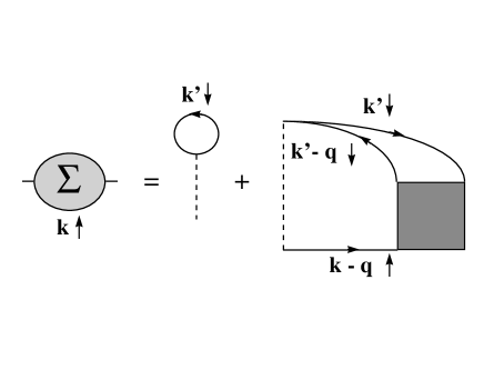
FIG. 1.: Formally exact diagrammatic representation of the self-energy in the Hubbard model. The square is the fully reducible four-point vertex

Many-body techniques of the paramagnon type[12] do lead to a pseudogap but they usually have low-temperature problems because they do not satisfy the Mermin-Wagner theorem. No such difficulty arises in the approach of Ref.[7]. This method proceeds in two stages. In the zeroth order step, the self-energy is obtained by a Hartree-Fock-type factorization of the four-point function with the additional constraint that the factorization is exact when all space-time coordinates coincide.[13] Functional differentiation, as in the Baym-Kadanoff approach [14], then leads to a momentum- and frequency-independent irreducible particle-hole vertex for the spin channel that satisfies[5] $U_{sp}=U\left\langle n_{\uparrow}n_{\downarrow}\right\rangle/\left(\left\langle n_{\uparrow}\right\rangle\left\langle n_{\downarrow}\right\rangle\right)$. The irreducible vertex for the charge channel is too complicated to be computed exactly, so it is assumed to be constant and its value is found by requiring that the Pauli principle in the form $\left\langle n_{\sigma}^{2}\right\rangle=\left\langle n_{\sigma}\right\rangle$ be satisfied. More specifically, the spin and charge susceptibilities now take the form $\chi_{sp}^{-1}\left(q\right)=\chi_{0}(q)^{-1}-\frac{U_{sp}}{2}$ and $\chi_{ch}^{-1}\left(q\right)=$ $\chi_{0}(q)^{-1}+\frac{U_{ch}}{2}$ with $\chi_{0}$ computed with the Green function $G_{\sigma}^{0}$ that contains the self-energy whose functional differentiation gave the vertices. This self-energy is constant, corresponding to the Hartree-Fock-type factorization.[15] The susceptibilities thus satisfy conservations laws,[14] the Mermin-Wagner theorem, as well as the Pauli principle $\left\langle n_{\sigma}^{2}\right\rangle=\left\langle n_{\sigma}\right\rangle$ implicit in the following two sum rules

$$\frac{T}{N}\sum_{q}\chi_{sp}\left(q\right) = \left\langle\left(n_{\uparrow}-n_{\downarrow}\right)^{2}\right\rangle=n-2\left\langle n_{\uparrow}n_{\downarrow}\right\rangle$$ (1)

$$\frac{T}{N}\sum_{q}\chi_{ch}\left(q\right) = \left\langle\left(n_{\uparrow}+n_{\downarrow}\right)^{2}\right\rangle-n^{2}=n+2\left\langle n_{\uparrow}n_{\downarrow}\right\rangle-n^{2}$$ (2)

where $n$ is the density. We use the notation, $q=\left({\bf q,}iq_{n}\right)$ and $k=\left({\bf k,}ik_{n}\right)$ with $iq_{n}$ and $ik_{n}$ respectively bosonic and fermionic Matsubara frequencies. We work in units where $k_{B}=1,$ $\hbar=1,$ lattice spacing and hopping $t$ are unity. The above equations, in addition to[5] $U_{sp}=U\left\langle n_{\uparrow}n_{\downarrow}\right\rangle/\left(\left\langle n_{\uparrow}\right\rangle\left\langle n_{\downarrow}\right\rangle\right)$, suffice to determine the constant vertices $U_{sp}$ and $U_{ch}$. This Two-Particle Self-Consistent approach will be used throughout this paper, unless we refer to FLEX calculations.

Once the two-particle quantities have been found as above, the next step of the approach of Ref.[7], consists in improving the approximation for the single-particle self-energy by starting from an exact expression where the high-frequency Hartree-Fock behavior is explicitly factored out. One then substitutes in the exact expression the irreducible low frequency vertices $U_{sp}$ and $U_{ch}$ as well as $G_{\sigma}^{0}(k+q)$ and $\chi_{sp}(q),\chi_{ch}(q)$ computed above. In the original approach[6] the final formula reads

$$\Sigma_{\sigma}^{\left(\ell\right)}(k)=Un_{-\sigma}+\frac{U}{4}\frac{T}{N}\sum_{q}\left[U_{sp}\chi_{sp}(q)+U_{ch}\chi_{ch}(q)\right]G_{\sigma}^{0}(k+q).$$ (3)

Irreducible vertices, Green functions and susceptibilities appearing on the right-hand side of this expression are all at the same level of approximation. They are the same as those used in the calculations of Eq.(1), hence they are consistent in the sense of conserving approximations. The resulting self-energy $\Sigma_{\sigma}^{\left(\ell\right)}(k)$ on the left hand-side though is at the next level of approximation so it differs from the self-energy entering the right-hand side.

There is, however, an ambiguity in obtaining the self-energy formula Eq.(3). Within the assumption that only $U_{sp}$ and $U_{ch}$ enter as irreducible particle-hole vertices, the self-energy expression in the transverse spin fluctuation channel is different. To resolve this paradox, consider the exact formula for the self-energy represented symbolically by the diagram of Fig.1. In this figure, the square is the fully reducible vertex $\Gamma\left(q,k-k^{\prime},k+k^{\prime}-q\right).$ In all the above formulas, the dependence of $\Gamma$ on $k+k^{\prime}-q$ is neglected since the particle-particle channel is not singular. The longitudinal version of the self-energy Eq.(3) takes good care of the singularity of $\Gamma$ when its first argument $q$ is near $\left(\pi,\pi\right).$ The transverse version does the same for the dependence on the second argument $k-k^{\prime}$, which corresponds to the other particle-hole channel. One then expects that averaging the two possibilities gives a better approximation for $\Gamma$ since it preserves crossing symmetry in the two particle-hole channels. Furthermore, one can verify that the longitudinal spin fluctuations in Eq.(3) contribute an amount $U\left\langle n_{\uparrow}n_{\downarrow}\right\rangle/2$ to the consistency condition[6] $\frac{1}{2}{\rm Tr}\left(\Sigma^{\left(\ell\right)}G^{0}\right)=$ $U\left\langle n_{\uparrow}n_{\downarrow}\right\rangle$ and that each of the two transverse spin components also contribute $U\left\langle n_{\uparrow}n_{\downarrow}\right\rangle/2$ to $\frac{1}{2}{\rm Tr}\left(\Sigma^{\left(t\right)}G^{0}\right)=$ $U\left\langle n_{\uparrow}n_{\downarrow}\right\rangle.$ Hence, averaging Eq.(3) and the expression in the transverse channel also preserves rotational invariance. In addition, one verifies numerically that the exact sum rule[7] $-\int d\omega^{\prime}\mathop{\rm Im}\left[\Sigma_{\sigma}\left({\bf k,}\omega^{\prime}\right)\right]/\pi=U^{2}n_{-\sigma}\left(1-n_{-\sigma}\right)$ determining the high-frequency behavior is satisfied to a higher degree of accuracy. As a consistency check, one may also verify that $\frac{1}{2}{\rm Tr}\left(\Sigma^{\left(t\right)}G^{\left(t\right)}\right)$ differs by only a few percent from$\frac{1}{2}{\rm Tr}\left(\Sigma^{\left(t\right)}G^{0}\right).$ We will thus use a self-energy formula that we call “symmetric”

$$\Sigma_{\sigma}^{\left(s\right)}(k)=Un_{-\sigma}+\frac{U}{8}\frac{T}{N}\sum_{q}\left[3U_{sp}\chi_{sp}(q)+U_{ch}\chi_{ch}(q)\right]G_{\sigma}^{0}(k+q).$$ (4)

$\Sigma_{\sigma}^{\left(s\right)}(k)$ is different from so-called Berk-Schrieffer type expressions[12] that do not satisfy[7] the consistency condition between one- and two-particle properties, $\frac{1}{2}{\rm Tr}\left(\Sigma G\right)=$ $U\left\langle n_{\uparrow}n_{\downarrow}\right\rangle.$

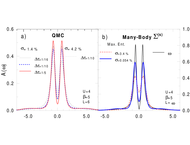
FIG. 2.: For $U=4$, $\beta=5$, $n=1$, ${\bf k}=(0,\pi)$, effect of various other calculational parameters: (a) QMC for $L=6$. Thick dotted line for $\Delta\tau=1/10$ and $\sigma=1.4\%$. The latter is the average of the error on $G(\tau)$ normalized by $G(\tau)$ itself. Calculations with the same $\sigma$ but for $\Delta\tau=1/5$ and $1/16$ are also shown. Thin dashed line is for $\Delta\tau=1/10$ but $\sigma=4.2\%$ on $G(\tau)$. (b) Thin solid line, real-frequency calculation using Eq.(4), for an infinite system. Also shown, Maximum Entropy inversion of $G(\tau)$ with same $\sigma$ as in Fig.3 and a smaller one.

In comparing the above self-energy formulas with FLEX, it is important to note that the same renormalized vertices and Green function appear in both the conserving susceptibilities and in the self-energy formula Eq.(4). In the latter, one of the external vertices is the bare $U$ while the other is dressed ($U_{sp}$ or $U_{ch}$ depending on the type of fluctuation exchanged). This means that the fact that Migdal’s theorem does not apply here is taken into account. This technique is to be contrasted with the FLEX approximation where all the vertices are bare ones, as if there was a Migdal theorem, while the dressed Green functions appear in the calculation. The irreducible vertex that is consistent with the dressed Green function is frequency and momentum dependent, contrary to the bare vertex appearing in the FLEX self-energy expression. In this Eliashberg-type self-consistent approach then, the Green functions are treated at a high level of approximation while all the vertices are bare, zeroth order ones. In other words, the basic elements of the perturbation theory are treated at extremely different levels of approximation.

III Monte Carlo vs many-body calculations

Our Monte Carlo results were obtained with the determinantal method[2] using typically $10^{5}$ Monte Carlo updates per space-time point. The inverse temperature is $\beta=5$, the interaction strength is $U=4$ and periodic boundary conditions on a square lattice are used. Other details about the simulations may be found in the captions. Our detailed analysis is for the single-particle spectral weight $A\left({\bf k,}\omega\right)$ at the wave-vector $k=\left(0,\pi\right)$ but other wave vectors will also be shown in the last figure of the paper. The Monte Carlo results are influenced by the statistical uncertainty, by the systematic error introduced through imaginary-time discretization, $\Delta\tau$, and by the finite size, $L$, of the system. The two calculations with $\Delta\tau=1/10$ in Fig.2a show that increasing the number of QMC sweeps (smaller $\sigma$, defined in Fig.2) leads to a more pronounced pseudogap. The same figure also shows calculations with the same $\sigma$ but different values of $\Delta\tau$ (systematic error is of order $\left(\Delta\tau\right)^{2}$). For $\Delta\tau\sim 1/10$, the decrease in pseudogap depth with decreasing $\Delta\tau$ becomes less than the accuracy achievable by the maximum entropy inversion. If the pseudogap persists when $L\rightarrow\infty$ at fixed $\sigma$ and fixed $\Delta\tau=1/10$ it should be even more pronounced with a larger number of QMC sweeps (smaller $\sigma$). The size analysis needs to be done however in more detail since increasing the system size $L$ at fixed $\sigma$ and $\Delta\tau$ leads to a smaller pseudogap, as shown on the top left panel of Fig.3a.

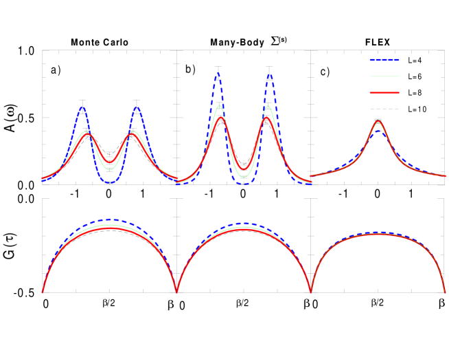
FIG. 3.: Size dependent results for various types of calculations for $U=4$, $\beta=5$, $n=1$, ${\bf k}=(0,\pi)$, $L=4,6,8,10$ and average relative errors $\sigma=3.4\%$ on $G(\tau)$. Upper panels show $A({\bf k},\omega)$ extracted from Maximum Entropy on $G(\tau)$ shown on the corresponding lower panels. Each $G(\tau)$ has $50$ points. (a) QMC. (b) Many-body using Eq.(4). (c) FLEX.

It is customary to analytically continue imaginary time QMC using the Maximum Entropy algorithm[11]. To provide a faithful comparison with the many-body approaches, we use the imaginary-time formalism for these methods and analytically continue them for the same number of imaginary-time points, using precisely the same Maximum entropy approach as for QMC. While the round off errors in the many-body approaches are very small, it is preferable to artificially set them equal to those in the corresponding QMC simulations to have the same degree of smoothing. Many-body results from the symmetric self-energy formula $\Sigma^{\left(s\right)},$ Eq.(4), for an infinite system are shown in Fig.2b. The thin solid line is a direct real-frequency calculation in the infinite-size limit. Maximum Entropy inversions of the $L\rightarrow\infty$ value of the many-body $G\left(\tau\right)$ shown on the same figure illustrate that with increasing accuracy the real-frequency result is more closely approximated. This confirms that Maximum Entropy simply smooths the results when artificially large errors are introduced in the analytical results.[16] For this parameter range, the effects are appreciable but do not change qualitatively the results. Even the widths of the peaks are not too badly reproduced by Maximum Entropy. The error bars are obtained from the Maximum-Entropy Bayesian probability for different regularization parameters $\alpha.$[11] They are clearly a lower bound.

In Fig.3, we show the spectra obtained for three techniques for system sizes $L=4,$ $6,$ $8$ and $10$. The left-hand panel is the QMC data, the middle panel is obtained from $\Sigma^{\left(s\right)}$ Eq.(4) while the last panel is for FLEX. The latter results for much larger lattices are not much different from those for the $8\times 8$ system. Since $G\left({\bf k,}\tau\right)=-\int\frac{d\omega}{2\pi}\frac{e^{-\omega\tau}}{e^{-\beta\omega}+1}A\left({\bf k},\omega\right),$ the nearly flat ($\tau$-independent) portion in $G\left({\bf k,}\tau\right)$ of the lower right-hand panel leads, in FLEX, to a maximum in $A\left(k,\omega\right)$ at $\omega=0,$ contrary to the Monte Carlo results. By contrast, as can be seen by comparing the middle and left panels, the agreement between Eq.(4) and QMC is very good, except for the height of the peaks. The finite-size dependence of the pseudogap for both QMC and Eq.(4) is similar: as the size increases, the depth of the pseudogap decreases. Some of the finite-size effects are present in the vertices $U_{sp}$ and $U_{ch}$.

Fig.4a compares three results for the $L=6$ system: QMC (thick solid line), and the many-body approach of Ref.[7] using either the symmetric $\Sigma^{\left(s\right)}$ (Eq.(4), dotted line) or the longitudinal $\Sigma^{\left(\ell\right)}$ (Eq.(3), thin solid line) self-energy formulas. In imaginary time, the agreement between QMC and $\Sigma^{\left(s\right)}$ is striking. The position of the peaks in QMC also agrees better with the symmetric version $\Sigma^{\left(s\right)}$, Eq.(4).

For the lattice sizes where the Monte Carlo data are qualitatively similar to those of Ref.[9], and hence uncontroversial, Fig.3 has shown that there is a many-body approach that gives good agreement with the simulations. Although this many-body approach is not rigorous, especially deep in the pseudogap regime where it is mostly an extrapolation method[7], these tests suggest that it can give an understanding of finite-size effects in QMC data. There are two intrinsic lengths that are relevant, namely $\xi$ the antiferromagnetic correlation length, and $\xi_{th}$ the single-particle thermal de Broglie wavelength defined by $v_{F}/T.$ In simulations, $\xi$ may be estimated from the momentum-space width of the spin structure factor and $\xi_{th}$ from the Fermi velocity estimated from the maxima of $A\left({\bf k},\omega\right)$ at different wave vectors. For $\beta=5,$ and $L=10$ we have $\xi\sim 3.$ At the $\left(\pi,0\right)$ point, $\xi_{th}$ essentially vanishes since we are at the van Hove singularity, hence the condition $L>\xi_{th}$ is satisfied. If we had $\xi_{th}>L,$ one would be effectively probing the finite-size zero-temperature quantum regime. When the condition $L>\xi_{th}$ is satisfied, as is the case here, one has access to the finite temperature effects we are looking for. Once agreement on the pseudogap in QMC and the analytical approach has been established up to the regime $\xi_{th}<L<\xi,$ the analytical approach [7] can be used to reach larger lattice sizes $\left(\text{such that }\xi_{th}<\xi<L\right)$ with relatively modest computer effort. In Fig.4b

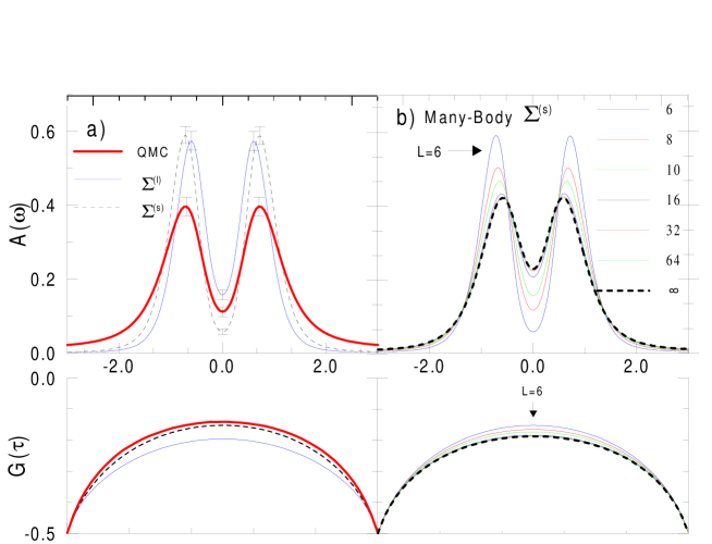
FIG. 4.: $U=4$, $\beta=5$, $n=1$, ${\bf k}=(0,\pi)$, and $\sigma=3.2\%$ in Maximum Entropy. (a) For $L=6$, thick solid line for QMC, and Many Body using two different self-energy formulas: dashed line for symmetric Eq.(4), and thin solid line for longitudinal Eq.(3). (b) Size dependent results obtained from symmetric version Eq.(4) for $L=6,8,10,16,32,64$ and infinite size (dashed line). The size dependence is monotonous.

we show the spectra obtained by Eq.(4) for $L=6$ to $64$ and then for $L=\infty$ (obtained from numerical integration). We see that the size dependence of the pseudogap becomes negligible around $L=32$ and that the pseudogap is quite sizable even though it is smaller than that in the largest size available in QMC calculations $\left(L=10\right).$ The size dependence of the pseudogap is qualitatively similar when the longitudinal form of the self-energy is used. We thus conclude that the pseudogap exists in the thermodynamic limit, contrary to the conclusion of Ref.[9]. The increase in QMC noise with increasing system size in the latter work may partly explain the different conclusion.

The last figure, Fig.5, shows $A\left({\bf k},\omega\right)$ obtained by Maximum Entropy inversion of Monte Carlo data (left panel) of the many-body approach Eq.(4) (middle panel) and of FLEX (right panel). Using the symmetry of the lattice and particle-hole symmetry, $A\left({\bf k},\omega\right)=A\left({\bf k+}\left(\pi,\pi\right),-\omega\right)$, one can deduce from this figure the results for all wave vectors of this $8\times 8$ lattice. The detailed agreement between Monte Carlo and the many-body approach is surprisingly good for all wave vectors, even far from the Fermi surface.

IV Discussion

There are two interrelated conclusions to our work. First, detailed analysis of QMC results along with comparisons with many-body calculations show that there is a pseudogap in the $n=1,d=2$ Hubbard model, contrary to results obtained from previous Monte Carlo simulations[9] and from self-consistent Eliashberg-type methods such as FLEX. Second, we have reinforced the case that the many-body methodology described here is an accurate and simple approach for studying the Hubbard model, even as we enter the pseudogap regime. While any self-energy formula that takes the form, $\Sigma\propto\sum_{q}\chi\left(q\right)G^{0}\left(k+q\right)$ will in general extrapolate correctly to a finite zero-temperature gap[17], and hence show a pseudogap as long as $\chi\left(q\right)$ contains a renormalized classical regime,[7] all other approaches we know of suffer from the following defects: they usually predict unphysical phase transitions, they do not satisfy as many exact constraints and in addition they do not give the kind of quantitative agreement with simulations that we have exhibited in Figs.3 to 5. Reasons why the mathematical structure of FLEX-type approaches fails to yield a pseudogap have been discussed before.[7] The same arguments apply to the pseudogap problem away from half-filling and for the attractive Hubbard model as well.[7, 8, 18, 19] Since in the Hubbard model there is no Migdal theorem to justify the neglect of vertex corrections, it is likely, but unproven, that to obtain a pseudogap in FLEX-type approaches, one would need to include vertex-correction diagrams that are at the same level of approximation as the renormalized Green functions.

The physical origin of the pseudogap in the 2D Hubbard model has been discussed at great length previously[7]: The precursors of antiferromagnetism in $A\left(k_{F},\omega\right)$ are preformed Bogoliubov quasiparticles that appear as a consequence of the influence of renormalized classical fluctuations in two dimensions. They occur only in low dimension when the characteristic spin relaxation rate is smaller than temperature and when $\xi/\xi_{th}>1$. With perfect nesting (or in the attractive Hubbard model) they occur for arbitrarily small $U.$ The ground-state gap value[20] (and corresponding single-particle pseudogap energy scale at finite $T$) depends on coupling in a BCS-like fashion.

The previous results show that strong-coupling local particle-hole pairs are not necessary to obtain a pseudogap. Such local particle-hole pairs are a different phenomenon. They lead to a single-particle Hubbard gap well above the antiferromagnetically ordered state, in any dimension but only when $U$ is large enough, in striking contrast with the precursors discussed in the present paper. The Hubbard gap also can exist without long-range order.[21]

From a methodological point of view, the strong-coupling Hubbard gap is well understood, in particular within the dynamical mean-field theory[22] or in strong-coupling perturbation expansion[23]. However, the precursors of Bogoliubov quasiparticles discussed in the present paper are unobservable in infinite dimension, where dynamical mean-field theory is exact, because they are a low dimensional effect. It remains to be shown if $1/d$ expansions or other extensions of infinite-dimensional methods will succeed in reproducing our results.[24]

Experimentally, one can distinguish a strong-coupling pseudogap from a precursor pseudogap (superconducting or antiferromagnetic) as follows. Ideally, if one has access experimentally to the critical quantity (spin or pair fluctuations) the difference between the two phenomena is clear since precursors occur only in the renormalized classical regime of these fluctuations. If one has access only to $A\left({\bf k},\omega\right),$ there are also characteristic signatures. The precursors are characterized by a “dispersion relation” that is qualitatively similar to that in the ordered state. (However the intensity of the peaks in $A\left({\bf k},\omega\right)$ does not have the full symmetry of the ordered state). By contrast, a strong-coupling pseudogap does not show any signs of the symmetry of the ordered state at high enough temperature.[21] Also, the temperature dependence of both phenomena is very different since precursors of Bogoliubov quasiparticles disappear at sufficiently high temperature in a manner that is strongly influenced by the Fermi velocity because of the condition $\xi/\left(v_{F}/T\right)>1$.[7, 19, 25] Hence, even with isotropic interactions, the precursor pseudogaps appear at higher temperatures on points of the Fermi surface that have smaller Fermi velocity, even in cases when the zero temperature value of the gap is isotropic. This has been verified by QMC calculations for the attractive Hubbard model.[8] By contrast, at sufficiently strong coupling, the Hubbard gap does not disappear even at relatively large temperatures, despite the fact that $A\left({\bf k},\omega\right)$ may rearrange over frequency ranges much larger than temperature.[26]

The methods we have presented here apply with only slight modifications to the attractive Hubbard model case where superconducting fluctuations[18] may induce a pseudogap[8, 19] in the weak to intermediate coupling regime relevant for the cuprates at that doping[27]. Recent time-domain transmission spectroscopy experiments[28] suggest that the renormalized classical regime for the superconducting transition in high-temperature superconductors has been observed. Concomitant peaks observed in photoemission experiments[29] persist above the transition temperature in the normal state. They may be precursors of superconducting Bogoliubov quasiparticles.[8] At exactly half-filling on the other hand, the paramagnetic state exhibits a strong-coupling (local particle-hole pairs) Hubbard gap.

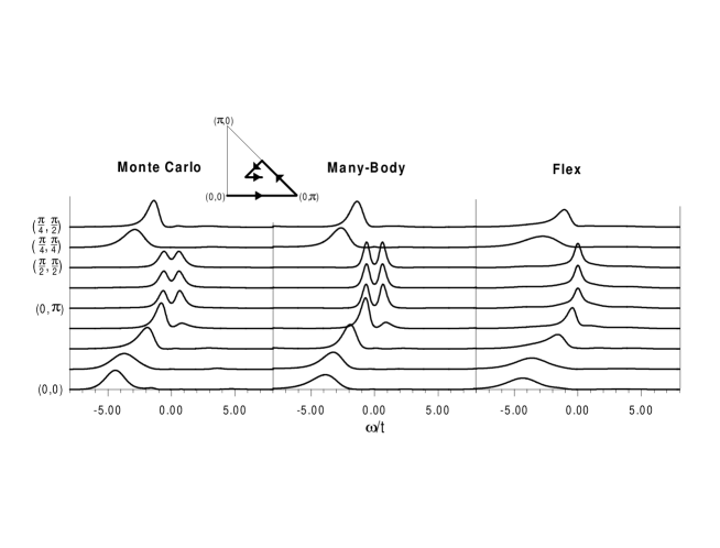
FIG. 5.: Single particle spectral weight $A({\bf k},\omega)$ for $U=4$, $\beta=5$, $n=1$, and all independent wave vectors ${\bf k}$ of an $8\times 8$ lattice. Results obtained from Maximum Entropy inversion of QMC data on the left panel and many-body calculations with Eq.(4) on the middle panel and with FLEX on the right panel. (Relative error in all cases is about 0.3%)

S.M. benefited from a useful correspondence with S. R. White. We thank J. Deisz for extended correspondence on this subject. Contributions to the code from H. Touchette are gratefully acknowledged. Monte Carlo simulations were performed in part on an IBM-SP2 at the Centre d’Applications du Calcul Parallèle de l’Université de Sherbrooke. This work was supported by a grant from the Natural Sciences and Engineering Research Council (NSERC) of Canada and the Fonds pour la formation de Chercheurs et l’Aide à la Recherche (FCAR) of the Québec government.

REFERENCES

- [1] J. E. Hirsh, Phys. Rev. B 31, 4403 (1985).
- [2] S. R. White, D.J. Scalapino, and R. L. Sugar, E. Y. Loh, Jr., J. E. Gubernatis, and R. T. Scalettar, Phys. Rev. B 40, 506 (1989).
- [3] N. E. Bickers and D. J. Scalapino, Annals of Physics, 193, 206 (1989); N. E. Bickers, D. J. Scalapino and S. R. White, Phys. Rev. Lett. 62, 961 (1989).
- [4] J. J. Deisz, D. W. Hess and J. W. Serene, Phys. Rev. Lett. 76, 1312 (1996).
- [5] Y.M. Vilk, Liang Chen, A.-M.S. Tremblay, Phys. Rev. B 49, 13 267 (1994).
- [6] Y. M. Vilk and A.-M. S. Tremblay, Europhys. Lett. 33, 159 (1996).
- [7] Y. M. Vilk and A.-M. S. Tremblay, J. Phys. I France 7, 1309 (1997).
- [8] S. Allen, H. Touchette, S. Moukouri, Y.M. Vilk, and A.-M. S. Tremblay, Phys. Rev. Lett. 83, 4128 (1999).
- [9] M. Vekic and S. R. White, Phys. Rev. B 47, 1160 (1993).
- [10] C. E. Creffield, E. G. Klepfish, E. R. Pike, and Sarben Sarkar, Phys. Rev. Lett. 75, 517 (1995).
- [11] M. Jarrell and J. E. Gubernatis, Phys. Rep. 269, 133 (1996). R. K. Bryan, Eur. Biophys. J. 18, 165 (1990).
- [12] N. Bulut, D.J. Scalapino, and S.R. White, Phys. Rev. B 47, 2742 (1993); N.F. Berk and J.R. Schrieffer, Phys. Rev. Lett. 17, 433 (1966).
- [13] This additional constraint leads to a degree of consistency between one- and two-particle quantities that is absent from the standard Hartree-Fock factorization.
- [14] Gordon Baym, Phys. Rev. B 127, 1391 (1962).
- [15] The constant self-energy is not equal to as it would in the trivial Hartree-Fock factorization (see previous note).
- [16] For small lattices, the many-body approach of Ref.[7] predicts many sharp peaks, as expected from the discreteness of the energy levels. Padé approximants with up to 512 Matsubara frequencies have great difficulties in reproducing these sharp features that are in any case smoothed out from the Monte Carlo data. Introducing artificially large random errors in the many-body technique in imaginary time and then applying Maximum Entropy has the effect of reducing the resolution in Care must be taken in choosing the errors. If they are too large they tend to broaden the spectra too much. We verified that for large system size the spectra obtained by Maximum Entropy are qualitatively similar to those obtained from Padé approximants.
- [17] S. Marcelja Phys. Rev. B 1, 2351 (1970).
- [18] S. Allen, B. Kyung and A.-M.S. Tremblay (unpublished)
- [19] Y.M. Vilk, S. Allen, H. Touchette, S. Moukouri, L. Chen and A.-M.S. Tremblay J. Phys. Chem. Solids 59, 1873 (1998).
- [20] The spin-density-wave ground state gap in is often refered to as a charge gap. It is a single-particle excitation gap. The spectral weight for the spin-spin correlation function has no gap because of the Goldstone modes. The spectral weight for the charge-charge correlation function is more complicated. When the spin order is co-linear, there is a gap to charge excitations, but when the order is spiral there can be no gap in the charge excitations, (even though the system is an insulator for DC current and there is a gap to single-particle excitations). In fact, in this case, for any wave vector other than zero the collective modes are a mixture of spin and charge excitations. See R. Côté and A.-M.S. Tremblay, Europhys. Lett. 29, 37 (1995).
- [21] However, close to the ordered state that appears at sufficiently low temperature at large some low energy feature may disperse with an energy scale but its distance from zero energy is of order
- [22] Antoine Georges, Gabriel Kotliar, Werner Krauth and Marcelo J. Rozenberg, Rev. Mod. Phys. 68, 13 (1996).
- [23] Stéphane Pairault, David Sénéchal, and A.-M. S. Tremblay, Phys. Rev. Lett. 80, 5389 (1998).
- [24] C. Huscroft, M. Jarrell, Th. Maier, S. Moukouri, A.N. Tahvildarzadeh, cond-mat/9910226. This work confirms our contention since by adding the effect of dimension through a cluster approach to dynamical mean-field theory, a pseudogap appears.
- [25] G. Preosti, Y. M. Vilk, and M. R. Norman , Phys. Rev. B 59, 1474 (1999).
- [26] D. Poulin, unpublished.
- [27] The model needs to be modified to obtain d-wave pairing.
- [28] J. Corson, R. Mallozzi, J. Orenstein, J.N. Eckstein, I. Bozovic, Nature, 398, 221 (1999); J. Corson, R. Mallozzi, J. Orenstein, J.N. Eckstein, I. Bozovic, cond-mat/9908368
- [29] A.V. Fedorov, T. Valla, P.D. Johnson, Q. Li, G.D. Gu, N. Koshizuka, Phys. Rev. Lett. 82, 2179 (1999).