Critical-point finite-size scaling in the microcanonical ensemble
Abstract
We develop a scaling theory for the finite-size critical behavior of the microcanonical entropy (density of states) of a system with a critically-divergent heat capacity. The link between the microcanonical entropy and the canonical energy distribution is exploited to establish the former, and corroborate its predicted scaling form, in the case of the 3d Ising universality class. We show that the scaling behavior emerges clearly when one accounts for the effects of the negative background constant contribution to the canonical critical specific heat. We show that this same constant plays a significant role in determining the observed differences between the canonical and microcanonical specific heats of systems of finite size, in the critical region.
PACS numbers: 05.20.Gg, 05.70.Jk, 64.60.Fr
I Introduction
Statistical mechanics can be formulated in any of a set of ensembles distinguished by the relationship between the system and its environment [1]. The principal members of this set are the microcanonical (prescribed energy) and canonical (prescribed temperature) ensembles. In the thermodynamic limit (when it exists) the ensembles yield the same predictions (and are, in this sense, equivalent) and the choice of ensemble is a matter of practical convenience. The canonical ensemble tends to win this contest because it circumnavigates the hard-constant-energy constraint imposed by the microcanonical ensemble.
The two ensembles are, however, not always equivalent [2]. They differ for systems which are ‘small’ in some sense: inherently small systems such as nuclei or clusters [3]; systems with unscreened long-range forces [4] where the thermodynamic limit is problematic; and systems at critical points [5], which are our principal concern here.
Theoretical studies of critical phenomena are almost invariably conducted within the framework of the canonical ensemble [6]. In consequence there is no substantive framework within which to interpret computational studies of microcanonical critical behavior. Such studies do, nevertheless, exist, having been motivated, variously, by the belief that the microcanonical framework may have some computational advantages [7] and by the discovery [8] that, apparently, critical anomalies in the microcanonical heat capacity are significantly enhanced with respect to their canonical counterparts.
This paper goes some way towards supplying the missing framework. We develop (section 2) a finite-size-scaling theory [9] for the microcanonical entropy (the density of states) of a system with a critically-divergent heat capacity. In so doing we have, of necessity, to consider more general questions about the structure of the density of states of a finite-size system –in particular the implications of well-established results for the finite-size structure of the canonical partition function [10].
Though somewhat more than a phenomenology, our theory falls short of being microscopically explicit: to determine an explicit form for the relevant scaling function we need to appeal (section 3) to Monte Carlo (MC) measurements of the critical canonical energy probability distribution (pdf).
The canonical energy pdf itself has a near-critical finite-size-scaling form which has featured in a number of studies of critical points in fluids [11] and lattice gauge theories [12]. Since energy fluctuations (like the critical anomaly in the canonical specific heat which they control) are relatively weak (by comparison with the fluctuations of the order parameter, and the divergence of its response function) the degree of ‘scaling’ reported in previously measured energy pdfs has been relatively poor –unsatisfactorily so for our purposes here. This problem is addressed in section 3. We show that one can fold out (from the measured distributions) the sub-dominant (but significant) non-scaling effects that are associated with the constant background contribution to the canonical heat capacity, negative in the case of the 3d Ising model [13]. This procedure exposes the underlying behavior, which manifests scaling to an impressive degree. In addition to providing us with the platform needed for this work, this procedure may offer the basis for improving the mixed-scaling-field theory [11] of critical points in systems that belong to the Ising universality class but which do not have full Ising symmetry; recent studies [12] have suggested that the current framework is not fully satisfactory.
The scaling form for the critical energy pdf allows us to determine the scaling form of the microcanonical entropy. In section 4 we explore this form and show that it is consistent with predictions for both the bulk-critical limit (as regards the parameters characterizing the specific heat singularity [13]) and the finite-size critical limit (the Fisher-Privman constant [14]).
The microcanonical entropy also provides us with a unified basis for dealing with both the canonical and the microcanonical specific heats (section 5). We show that the ‘corrections’ to the scaling behavior of the canonical specific heat (the negative background constant) have subtle consequences for the microcanonical behavior. In particular they serve to amplify the difference between microcanonical and canonical behavior, and are at least partially responsible for the strength of the anomaly observed in some microcanonical studies [8].
A The microcanonical scaling ansatz
We consider a d-dimensional many-body system of linear dimension ; we assume hypercubic geometry with periodic boundary conditions. The canonical partition function is, in principle, a discrete sum over system microstates () or system energy levels ():
| (1a) |
where is the degeneracy of level . We shall suppose that the system is sufficiently large that the sum over levels can be replaced by an integral:
| (1b) |
where is the energy density. The function is the density of states; as we have defined it, it is a true density, having dimensions of inverse energy. We note that the transition from the discrete representation (Eq. 1a) to its continuum counterpart (Eq. 1b) requires some care: it is discussed in Appendix A.
Our microcanonical scaling theory comprises a proposal for the form of the density of states function. We formulate it in two stages. Consider first a regime remote from critical points or lines of phase coexistence. In such a regime we make the general finite-size ansatz [15]:
| (2) |
The structure proposed for the prefactor makes this a little more than simply a definition of the microcanonical entropy density . In its support we note, first, that one may readily verify it explicitly (Appendix B) in the case of some simple model systems. Secondly we note the implications for the associated canonical partition function. Inserting Eq. (2) into Eq. (1b), a saddle-point integration gives
| (3) | |||||
| (4) |
where
| (5) |
and is the solution of
| (6) |
Eq. (4) recovers the prefactor-free form of the canonical partition function believed to be widely appropriate in regions (those where the saddle point integration is to be trusted) remote from critical points or lines of phase coexistence [10]. We note that this form is achieved by virtue of the prefactor that does appear in the density of states ansatz (Eq. 2), which is just such as to cancel the contributions made by the fluctuations about the saddle point [16].
The argument we have given leaves open the possibility of power-law corrections to Eq. (4). It has long been believed, and more recently established rather generally [10], that the corrections to the leading form are actually exponentially small in the system size. Since the saddle-point integration necessarily generates power-law corrections, one must suppose that there are compensating power-law corrections to the ansatz (Eq. 2) for the density of states. This conclusion serves as a warning (already suggested by the double appearance of the function in Eq. (2)) that the microcanonical framework faces problems which are skirted in the canonical formalism [17].
Now, more specifically, consider a system, of the kind specified above, in the vicinity of a critical point. We will suppose that the critical point has a divergent heat capacity; where we need to be more specific we shall assume it is a member of the d=3 Ising universality class (or, more specially still, the d=3 Ising model itself). Within the microcanonical framework the critical point of such a system is located by a critical value of the energy density, sharply-defined in the thermodynamic limit. We are concerned with the behavior of the microcanonical entropy for energies in the vicinity of this critical value. To describe this regime we introduce the dimensionless scaling variable [18]
| (7) |
where is an appropriate scale factor and the index is defined by
| (8) |
with the index (assumed positive) characterizing the heat capacity divergence, and the correlation length index [19]. We now reformulate and extend our basic ansatz (Eq. 2) with the proposal that, in a region of sufficiently large and sufficiently small [20]
| (9a) |
with
| (9b) |
Here is an unimportant constant, is the critical inverse temperature and is a finite-size-scaling function, universal given some convention on the scale factor , introduced in Eq. (7). The remainder of this paper is devoted to providing support for this proposal, and exploring the structure of the microcanonical entropy scaling function which it introduces.
II Determining the scaling function
It should be possible to determine the finite-size-scaling function within the renormalization group framework [21]. We have not done that. Instead we have chosen to learn what we can about this function from its signatures in MC studies of the canonical ensemble.
Consider, then, the implications of the scaling form Eq. (9b) for the canonical partition function, Eq. (1b). We suppose initially (we shall have to refine the supposition, shortly) that the relevant part of the energy spectrum is adequately captured by Eq. (9b). Then
| (10) |
where
| (11) |
and
| (12) |
while
| (13) |
provides a scaling measure of the deviation from the critical temperature. We have made use of the hyperscaling relation [19] which links the correlation length index and the heat capacity index through
| (14) |
The scaling form of the free energy follows:
| (15) |
The canonical energy pdf
| (16) |
may also be written in scaling form:
| (17) |
with
| (18) |
The scaling predictions for the pdf may be tested by examining its cumulants [22], for which the free energy is a generator:
| (19) |
Eq. (15) then implies that the cumulants have the scaling form
| (20) |
where the scaled cumulants are universal functions:
| (21) |
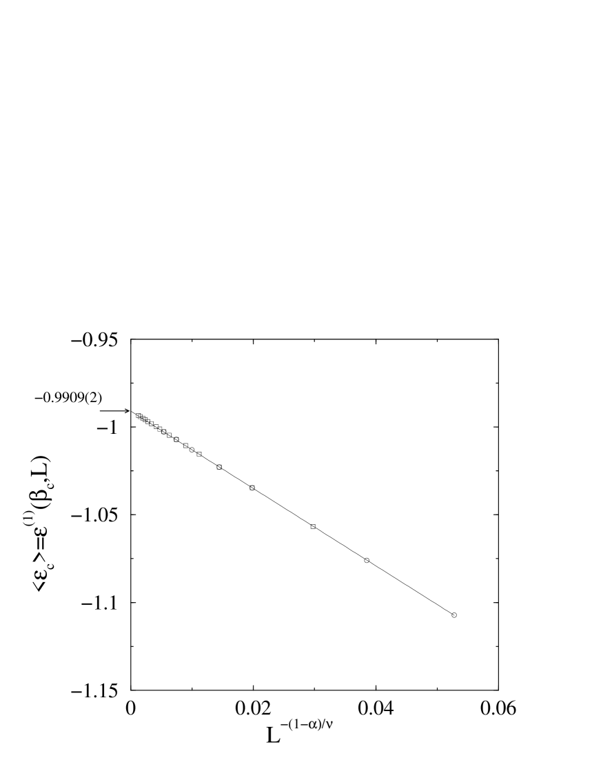
The canonical mean of the energy density at criticality () follows as:
| (22) |
MC measurements on the 3d Ising model using a range of system sizes (Fig. 1) are fully consistent with this behavior.
Eq. (15) implies, likewise, that the canonical variance of the energy density should have the power law behavior
| (23) |
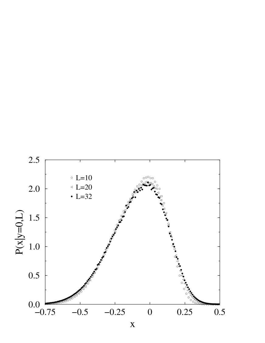
MC measurements (Fig. 2) are only partially consistent with this prediction: the power law is confirmed, but with an extrapolation whose intercept is far from zero. This inconsistency is reflected in the rather limited success (Fig. 3) of attempts to collapse the measured energy pdfs for different system sizes on to a single scaling form. The source of these problems can be guessed from the implications of Eq. (23) for the canonical specific heat, which it mirrors: the scaling form fails to capture the effects associated with the constant background which constitutes the dominant correction to pure scaling (power-law divergence) of the canonical specific heat.
There are two ways to rectify this failure. One might extend the theory to predict the behavior of the (very) finite systems accessible to MC study; or one might seek to correct the MC results to expose the true scaling behavior. We adopt the latter strategy.
Define
| (24) |
the difference between the true free energy density and its asymptotic scaling form (see Eq. (15)). We shall ignore the effects of confluent singularities: they are not the dominant ‘corrections to scaling’ here. Then is analytic and may be approximated, near , by the expansion
| (25) |
These additional contributions to the free energy imply additional contributions to the energy cumulants (Eq. 19):
| (26) |
At criticality Eq. (20) must then be modified to read
| (27) | |||||
| (28) |
where
| (29) |
The correction is absent by fiat: the choice of ensures this. The corrections are sufficiently strongly ‘irrelevant’ (they vanish sufficiently strongly with ) that they may reasonably be neglected. But the correction decays only slowly:
| (30) |
where the last step defines (a convenient parameter) while
| (31) |
is identifiable as the constant ‘background’ to the near-critical canonical specific heat. With this addition, Eq. (23) is modified to read
| (32) |
which is now fully consistent with the MC measurements of Fig. 2, with (it is to be noted) a negative value for [23]. From a thermodynamic point of view these results simply reflect the fact that, for any system size practically accessible to computer-simulation, the ‘critical’ contribution to the canonical specific heat is not large enough to dominate the ‘non-critical background’. But the argument also shows us how to eliminate the effects of this ‘background’ from the energy pdf.
Consider the cumulant representation [22] of the scaling energy pdf (Eq. 18) at criticality:
| (33) |
The corresponding relation for the observed energy pdf at criticality, written in its inverse form, is
| (34) |
Appealing to the our conclusion that, for large enough , the cumulants of the two pdfs differ significantly only in the case, and using Eqs. (29) and (30), we find that
| (35) | |||||
| (36) |
This result shows that the scaling form of the critical pdf may be exposed by convolution of the observed (and thus, generally, non-scaling) pdfs with gaussians whose widths are controlled by the specific heat background. Note that the argument rests on the fact that this background is negative (so that as defined in Eq. (30) is positive). If the background constant were positive our argument would have to be restructured to prescribe the scaling form by a process of deconvolution, which is numerically problematic. As it is, the convolution process can be implemented easily. With fixed by the ordinate intercept in Fig. 2, the pdfs measured on different system sizes can each be corrected in this way to yield estimates of the scaling pdf. The results are shown in Fig. 4. The improvement with respect to the raw data (Fig. 3) is striking. This improvement reflects not only the removal of the non-scaling contribution to the second cumulant but also that the requisite convolution process provides a natural smoothing of the MC data [28]. The consequences of this correction for the shape of the distribution are also striking. The skewness [29] clearly visible in the raw distributions (Fig. 3) is largely suppressed to expose a scaling form that is, at first appearance, gaussian. Indeed the portion of the distribution evident on the scale of Fig. 4 is gaussian to within deviations of a few per cent. However the behavior in the wings (evident on the logarithmic scale utilized in Fig. 5) is markedly different on the high- and low-energy sides.
The scaling of the critical energy pdf corroborates the scaling of the microcanonical entropy (cf Eq. (18)). Given the double appearance of in Eq. (18) it is practical to infer only the ‘effective’ microcanonical entropy scaling function
| (37) |
Fig. 5 shows the form implied by Eq. (18)
| (38) |
We note as a matter of empirical fact that is concave. The concavity of itself is already assumed in our basic scaling ansatz [15].
III The scaling theory: implications and tests
Although we have no first-principles calculation of the scaling function to offer here we can identify, and test, some of the properties it must have to match anticipated behavior in both the thermodynamic and finite-size-critical limits.
We consider, in particular, the limiting large behavior. In this regime we anticipate that
| (39) |
where the and subscripts refer, respectively, to the regions of positive and negative . To make explicit identifications of the new quantities introduced in this equation (the exponent and the amplitudes , ), consider the scaling part of the partition function (Eq. 12). In the limit of large the integral in Eq. (12) is dominated by one or other of the large regimes. Substituting Eq. (39), a saddle-point integration yields
| (40) |
where the and subscripts now refer, respectively, to the regions of negative and positive [30], and
| (41) |
As in the argument leading to Eq. (4) the fluctuations about the saddle point are canceled by the pre-exponential factor in Eq. (12) to leave power-law (‘ln-free’) behavior [31].
The thermodynamic limit of the near-critical free energy, defined by Eq. (15), now follows as
| (42) |
where we have identified
| (43) |
and (given Eq. 41)
| (44) |
To establish the role of the remaining constants () in Eq. (39) we consider the anomalous contribution to the free energy [14] defined by
| (45) |
Appealing to Eq. (42), and recalling our sign convention [30], we identify
| (46) |
On the basis of rather general arguments [10] we expect that away from a critical point the free energy anomaly is just minus the logarithm of the number of coexisting phases, so that
| (47a) | |||||
| (47b) |
In the critical finite-size limit we find from Eq. (15)
| (48) |
The critical value of the free energy anomaly, defining the Privman -Fisher constant [14], follows as
| (49) |
These predictions are testable to varying degrees through both the energy-dependence of the energy pdf and the temperature-dependence of the associated free energy.
Figure 6 shows the results for the ratio of the specific heat amplitudes that follow from Eq. (44) when the measured decay of the critical energy pdf (Figs. 4, 5) is matched to the prediction (39), in conjunction with Eq. (18). We can expect the predictions and observations to match up only in a window of values. Clearly, must be large enough to lie within the thermodynamic critical region; but it must also not be so large that the associated energy lies outside the domain of validity of the basic scaling ansatz (Eq. 9b). The size of this window should increase with increasing system size. The location of this window on the -axis may also be expected to be different for the positive and negative -branches –if, as seems reasonable, one regards the correlation length (rather than or ) as a measure of criticality. This is, indeed, the view we have adopted [33]. Thus Fig. 6 shows the results for the ‘effective’ amplitude ratio, obtained by fitting over ranges of values, with each pair of (positive and negative ranges) being centered on the same value of , used as the abscissa [32]. On the basis of this data [34] we make the assignment which is to be compared with in reference [13] and in reference [25].
In Fig. 7 we show the results for that follow (cf Eqs. (12), (37), (38)) from the measured energy pdfs, using Eq. (38). The latter determines only to within an additive constant which must be fixed by appeal to the predicted value of either or . We have chosen the latter so that Eq. (47b) is satisfied, by fiat. The motivation for this choice is that it provides us with an inherently more reliable estimate of the parameter (which, unlike , is not known a priori). Since is closer to than to the function converges more quickly to its asymptote than it does to its asymptote. Fixing (the intercept of the asymptote) thus tethers the value assigned to more effectively than fixing . As with the amplitude ratio considered above, the value assigned to depends upon the range of -values used in the fit to the anticipated asymptotic form (Eq. 40). Again we have chosen to characterize the temperature range utilized through the value of the ratio ; again we can expect the analysis to be trustworthy only if it is based upon data lying within the thermodynamic-critical window. Our data (Fig. 8) do not allow a systematic analysis of the approach to the desired limit; but they provide the basis for the assignment [34]. The assignment of the uncertainty limit is subjective but, we think, conservative. We note the close correspondence with the assignment () emerging from an earlier study [36], similar in concept, but utilizing the distribution of the order parameter. However our assignment differs (in what would seem to be a statistically significant fashion) from the result obtained by Mon [35] on the basis of altogether different techniques.
IV Microcanonical and canonical specific heats
A Generalities
Thus far we have focused on the implications of the microcanonical entropy for observations made in the canonical ensemble. We now turn to consider their implications for observations made within ensembles that are (or are approximations to) microcanonical.
We will assume (in keeping with eg [2, 8]) that the temperature of a microcanonical system should be identified from the relation
| (50) |
This identification is certainly required in the thermodynamic limit; but in the context of systems of finite size it is, it seems, a matter of convention [37].
It is illuminating to link this temperature with canonical observables. Appealing to Eq. (16) we may write
| (51) |
where (notwithstanding appearances to the contrary) the rhs depends on but not . This result shows that the equation prescribing the microcanonical temperature for a given energy is just the inverse of the equation prescribing the most probable energy for a given temperature:
| (52) |
By comparison, within the canonical ensemble itself, ‘the’ energy for a given temperature is customarily identified with the canonical mean:
| (53) |
Eqs. (52) and (53) make it immediately plain that the energy-temperature relationships associated with the two ensembles will coincide to the extent that the canonical energy distribution is gaussian (and thus has coincident mean and mode ). This correspondence is guaranteed in the thermodynamic limit, but not (in general) when finite-size effects are significant.
The energy-temperature relationships are most usually probed through their derivatives, the associated specific heats. In the microcanonical case
| (54) |
where, again, the -dependence of the rhs is illusory.
In the canonical case (appealing to Eq. (19))
| (55) |
B Scaling forms
First, we examine the asymptotic scaling regime where the the ‘background’ contribution to the specific heat can be neglected. We will consider the consequences of the corrections associated with the latter in the following section.
In the scaling regime where the canonical energy pdf may be represented by its scaling form (Eqs. (17) and (18)) Eq. (51) can be rewritten in terms of the energy and temperature scaling variables (Eqs. (7) and (13)) as
| (56) |
where in the last step we have exercised the right to set (the result is independent of ) and have made use of Eqs. (18) and (37). The microcanonical specific heat (Eq. 54) follows in scaling form
| (57a) |
with
| (57b) |
The scaling form of the canonical specific heat follows in a similar fashion, using Eqs. (20) and (55)
| (58a) |
with (Eq. 23)
| (58b) |
The forms of both the scaling functions and can be determined from the scaling form for the microcanonical entropy (Fig. 5) or, equivalently, the critical canonical energy pdf (Fig. 4), established in the preceding section. They are compared in Fig. 9. In the microcanonical case we have used Eq. (56) to identify the microcanonical temperature to be associated with a given value of the energy variable .
In the thermodynamic limit realised at large values of the two functions are, necessarily, consistent with one another, and approach the asymptotic behavior implied by Eq. (42). In the finite-size-critical (small ) regime, however, clear differences between the two scaling forms are apparent. In particular, the microcanonical maximum exceeds the canonical maximum by some . One can show (Appendix C) that this –the fact that the microcanonical maximum is the larger one– follows necessarily if the scaling function is concave.
The two scaling functions cross very close to the point () identifying the bulk critical temperature. One can see this already in published microcanonical data [8]; a similar ‘ensemble-independence’ has also been noted in studies of the ‘gaussian ensemble’ [38]. We have been unable to see any deep reason for this correspondence; but we do not discount the possibility that there is one.
Though clearly visible, the differences between the two scaling functions are smaller than suggested by existing MC data [8]. The next section explains why.
C Beyond scaling: the role of the ‘background’
To understand the behavior observed in MC studies of microcanonical behavior, we must allow for the ‘corrections to scaling ’ which, in the canonical ensemble, are reflected simply in the existence of the additive negative background contribution to the heat capacity; their signature in the microcanonical ensemble is more subtle.
The differences between the canonical and microcanonical results is effectively a strongly anharmonic effect: in a system of finite size, critical fluctuations sample a region of the entropy surface sufficiently large that the variation of its curvature becomes significant. We can expose the consequences analytically within an anharmonic perturbation theory in the cumulants of the energy pdf. The calculation is straightforward and we describe it in outline only.
We appeal to the cumulant representation of the energy pdf at some (general) temperature:
| (59) |
We expand perturbatively to first order in the fourth cumulant and to second order in the third. We evaluate the second derivative of the logarithm of this function, which determines (cf Eq. (54)) the microcanonical specific heat associated with a given energy density. We evaluate this function at the modal energy associated with the chosen temperature, prescribed by the (perturbative) solution of the microcanonical caloric equation of state (Eq. 51). The result is
| (60) |
Eq. 19 shows that the cumulant correction terms displayed in this equation are in the thermodynamic limit, confirming the equality of microcanonical and canonical predictions in this limit. To see what happens in the finite-size-critical region we focus (for simplicity) on the temperature for which the canonical specific heat is maximal, identified by the solution of
| (61) |
At this temperature Eq. (60) simplifies to
| (62) |
where , and we have used Eq. (55). Now we appeal to the scaling forms for the cumulants (Eq. 20), and fold in the effects of the additional non-scaling contribution to the second cumulant (Eq. 30) to conclude that
| (63) |
This result makes clear (albeit perturbatively) that, in the finite-size-limited regime, the temperature-independent additive ‘background constant’ in the canonical specific heat (manifested in the parameter ) does not simply translate into an additive energy-independent background in its microcanonical counterpart.
To expose the implications for the difference between canonical and microcanonical specific heats we introduce the dimensionless parameter:
| (64) |
Then
| (65) |
where is the scaling limit of .
The significance of the background constant –in particular, its sign– is now apparent. The negative value of this constant results in an amplification of the difference between the microcanonical and canonical results (at ), to a degree that diminishes with increasing system size. This is not simply the trivial effect that would arise from a uniform (downward) shift of both functions: Eq. (63) shows that this is not what happens, as does the power of two on the rhs of Eq. (65).
It is not hard to track down the origins of this effect. The difference between the canonical and microcanonical specific heats is, we have noted, an anharmonic effect; in the present context the ‘corrections to scaling’ reduce (only) the second cumulant of the energy pdf and thus, in a relative sense, enhance the anharmonic (non-gaussian) character of the energy pdf, as one can see immediately from a comparison of Figures 3 and 4.
V Conclusions
We review, briefly, the three principal strands of this work.
First, we have broached the general question of the finite-size corrections to the density of states of a many-body system. The explicit proposal for the pre-exponential structure advanced in Eq. (2) is consistent with the pre-factor-free structure of the canonical partition function [10] and with the behavior of the simple models discussed in Appendix B. Given the growing interest in the behavior of mesoscopically-sized systems, this proposal seems to merit some further study, with more rigor than we have attempted to offer here.
Second, we have shown how one can fold out from the canonical energy fluctuation spectrum the principal corrections to scaling. The underlying behavior exhibits scale-invariance to a degree that seems remarkable, given the relative weakness of energy fluctuations. It is, we have seen, also largely consistent with established 3d-Ising critical properties.
Third, we have provided a finite-size scaling theory of the microcanonical ensemble. This was the original motivation for this work– specifically, the suggestion [8] that the finite-size-smearing of critical behavior characteristic of the canonical ensemble is ‘greatly reduced’ within the microcanonical framework. Reference [8] offers two pieces of supporting evidence for this contention, which merit final comment.
Reference [8] suggests, firstly, that, in the vicinity of , the microcanonical entropy (measured with the techniques described in [40]) can be adequately represented by a form (Eq. 6 of reference [8]) which allows for no finite-size corrections at all, and which corresponds essentially to the large limit (Eq. 39) of our scaling function. In fact the quality of the fit provided by this representation is rather poor. And we would expect it to be so. The measured microcanonical entropy evolves in a manifestly smooth way [41] between the limiting thermodynamic forms appropriate above and below ; Eq. 6 of reference [8] is non-analytic at . Moreover, in analyzing data for the entropy and its derivatives, it is – we have seen – essential (on all systems practically accessible) to do justice to the corrections associated with the background constant . Even in the thermodynamic limit the corrections allowed for in Eq. (8) of reference [8] do not do this.
The second piece of supporting evidence offered in reference [8] is a striking enhancement of the critical peak in the microcanonical specific heat, with respect to its canonical counterpart. As we have seen, this behavior is at least partly due [42] to the effects associated with ; Figure 9 indicates that the underlying differences are rather less dramatic.
ACKNOWLEDGMENTS
NBW acknowledges the financial support of the Royal Society (grant no. 19076), the EPSRC (grant no. GR/L91412) and the Royal Society of Edinburgh.


REFERENCES
- [1] See for example T.L. Hill, Statistical Mechanics (McGraw-Hill, 1956).
- [2] D.H.E. Gross, Physics Reports 279, 119 (1997).
- [3] X.Z Zhang, D.H.E. Gross S.Y. Yu & Y.M. Zheng, Nucl. Phys A 461, 668 (1987).
- [4] W. Thirring, Z. Phys. 235, 339 (1970).
- [5] R.C. Desai, D.W. Heermann & K. Binder, J. Stat. Phys. 53, 795 (1988).
- [6] This choice reflects the belief that ‘fields’ rather than ‘densities’ provide the natural coordinates of the critical region: see M.E. Fisher, Phys. Rev. 176, 257 (1968).
- [7] M. Creutz, Phys. Rev. Lett. 50, 1411 (1983).
- [8] M. Promberger & A. Hüller, Z. Phys. B97, 341 (1995).
- [9] For a review of finite size scaling see Finite Size Scaling and Numerical Simulation of Statistical Systems, edited by V. Privman (World Scientific Publishing, Singapore, 1990).
- [10] C. Borgs and R. Kotecký, J. Stat. Phys. 61, 79 (1990); Phys. Rev. Lett. 68, 1734 (1992).
- [11] A.D. Bruce and N.B. Wilding, Phys. Rev. Lett. 68, 193 (1992); N.B.Wilding and A.D.Bruce, J.Phys: Condens. Matter 4, 3087 (1992); N.B. Wilding, Phys. Rev. E 52, 602 (1995).
- [12] K. Rummukainen, M. Tsypin, K. Kajantie, M. Laine & M. Shaposhnikov Nuclear Physics B 532, 283 (1998).
- [13] A.J. Liu & M.E. Fisher, Physica 156, 35 (1989).
- [14] V. Privman and M.E. Fisher, Phys. Rev. B 30, 322 (1984).
- [15] Eq. (2) assumes that the entropy density is concave, so that is positive. This concavity condition is guaranteed only in the thermodynamic limit. It is violated in the two phase region of a finite-sized system exhibiting a first order phase transition with a latent heat. See eg A. Hüller, Z. Phys B. 95, 63 (1994). In these circumstances Eq. (2) cannot be correct.
- [16] Compare Eqs. (2) and (4) with equations 3.3 and 3.7 in reference [2].
- [17] Such problems are already apparent, for example, in the correlations induced in ideal gases by the microcanonical energy constraint: see eg J.L Lebowitz and J.K. Percus, Phys. Rev. 124, 1673 (1961).
- [18] We assume that our Ising system has the full (‘particle-hole’) symmetry of the Ising model itself. In those cases [11, 12] which fall into the Ising universality class but do not have this symmetry one must allow for scaling-field-mixing: see [11] and references therein. We expect that the key results of the present work —notably the scaling ansatz for the density of states (Eq. 8)— remain applicable provided the scaling energy density defined in Eq. 7 is replaced with an appropriate linear combination of the energy density and the density of the ordering variable (eg the particle density in the case of a fluid). The generalisation of our analysis to incorporate simultaneous ‘microcanonical’ constraints on both energy and ordering density is beyond the scope of the present work.
- [19] See for example M.E. Fisher, Rep. Prog. Phys. 30, 615 (1967).
- [20] We will use to signify equality in such an asymptotic sense.
- [21] E. Brézin and J Zinn-Justin, Nucl. Phys. B 257 (FS14), 867 (1985).
- [22] H. Cramer, Mathematical Methods of Statistics (Princeton University Press, Princeton, 1946).
- [23] See reference [13]. The results of that paper indicate that the range of reduced temperatures below criticality (), in which the subdominant ‘background’ contribution to the specific heat is effectively constant, is small.
- [24] The Ising system energy is measured in units of the coupling constant .
- [25] M. Hasenbusch and K. Pinn, J.Phys. A: Math. Gen. 31, 6157 (1998).
- [26] H.W.J. Blöte, E Luitjen & J.R. Herringa, J.Phys. A: Math. Gen. 28, 6289 (1995).
- [27] A.M. Ferrenberg and R.H. Swendsen, Phys. Rev. Lett. 63, 1195 (1989); R. H. Swendsen, Physica A 194, 53 (1993).
- [28] Note, in contrast, that the procedures adopted in reference [8] require a phenomenological smoothing of raw estimates of the microcanonical entropy, with results that depend sensitively upon the values chosen for the smoothing parameters.
- [29] This skewed energy distribution has appeared (without finite-size-scaling analysis) in a number of papers: see for example Figure 1 of N.A. Alvez, B.A. Berg & R. Villanova, Phys. Rev. B 41, 383 (1990); Figure 2 of A.M. Ferrenberg & D.P. Landau, Phys. Rev. B 44, 5081 (1991).
- [30] The sign convention for the subscripts is chosen to match the conventions of critical phenomena, where amplitudes are labeled according to the sign of rather than .
- [31] The pre-exponential factor also leads to a power-law modulation of the exponential decay of the energy pdf, in the large regime. Our data provides no significant direct support for this term. The existence of such a term in the pdf of the order parameter has been noted by many authors, and is relatively well established: see [21], [36] and G.R. Smith & A.D. Bruce, J. Phys. A: Math. Gen. 28, 6623 (1995); M.M. Tsypin, e-print hep-lat/9401034; J. Rudnick, W. Lay & D Jasnow, Phys. Rev. E 58, 2902 (1998).
- [32] The conversion between , and scales uses the amplitudes (of correlation length and specific heat singularities) assigned in reference [13].
- [33] The tuning of the choice of high-temperature series-expansion-variable in reference [13] has qualitatively similar consequences for amplitude-ratio-determination.
- [34] Note that this assignment (including its uncertainty) is conditional upon the choices of the other parameters specified in the caption to Fig. 1.
- [35] K.K. Mon, Phys. Rev. B 39, 467 (1989).
- [36] A.D. Bruce, J. Phys. A: Math. Gen. 28, 3345 (1995).
- [37] See for example B.B. Mandelbrot, Physics Today 42, 71 (1989).
- [38] M.S. Challa & J.H. Hetherington, Phys Rev A 38, 6324 (1988).
- [39] J.R. Ray & C. Frelechoz, Phys. Rev. E 53, 3402 (1996). Note that, in common with others, these authors impose the microcanonical constant energy constraint on a system comprising the intrinsic (Ising spin) degrees of freedom and a set of artificial conjugate momenta.
- [40] G.R. Gerling and A. Hüller, Z. Phys B 90, 207 (1993).
- [41] If plotted as a function of the entropy displays an effectively straight line section (as it does at a first order phase transition) extending over an interval (in which ) that grows as –in contrast to a first-order transition where the interval grows as . This bears out a conjecture by L Stodolsky and J Wosiek, Nucl. Phys. B 413, 813 (1994).
- [42] Note that the sharpness of the microcanonical peak reported in Fig. 1 of [8] is also heavily dependent upon the parameters of the smoothing procedure used there: see [28].
- [43] See for example F Reif, Fundamentals of statistical and thermal physics (McGraw-Hill, New York, 1965) p61, being wary of the notational differences.
- [44] I.S. Gradshteyn & I.M. Ryzhik, Table of integrals, series and products (Academic Press, New York, 1980).
- [45] M.N. Barber & M.E. Fisher, Ann. Phys. 77, 1 (1973).
A Defining a density of states
We discuss here, in general terms, the issues arising in defining a density of states function for a system in which the energy spectrum is discrete. The conventional argument [43] makes the identification
| (A1) |
with the implicit assumption that the right hand side is proportional to (). This requires that:
-
[C1]
There exist many distinct levels within the interval .
-
[C2]
The level degeneracy is slowly varying over the interval .
The fractional variation of over the interval can be estimated using Eq. (50); condition C2 can then be expressed in the form
| (A2) |
Taken together, conditions C1 and C2 thus amount to the requirement that
| (A3) |
where characterizes the intrinsic discreteness of the energy spectrum. This condition is trivially satisfied in the classical limit (Appendix B1 considers one case explicitly). But there are obvious exceptions: in the Ising model (Appendix B2) Eq. (A3) is satisfied only at energies corresponding to microcanonical temperatures that are ‘high’ on the scale of the critical temperature. Or, to put it another way, is certainly not slowly varying over a range wide enough to embrace many system energy levels. We must now recognize, however, that Eq. (A1) (along with its implicit assumptions) does not faithfully reflect the conditions needed to legitimize the transition from discrete (Eq. 1a) to continuum (Eq. 1b) representations. Instead of Eq. (A1) we require, rather, that we can consistently write
| (A4) |
where (while retaining condition C1) we must replace condition C2 by
-
[C2A]
is slowly varying over the interval , if that interval lies in a range contributing significantly to the thermal properties at temperature .
The range contributing significantly … is centered on the saddle point (Eq. 6). As a result, while condition C2 requires Eq. (A2), condition C2A requires only that
| (A5) |
where we have used Eq. (54). Thus, in place of Eq. (A3), we need simply
| (A6) |
where the last step uses Eq. (55), and (Eq. 50). This equation expresses more explicitly the implications of condition C2A. A density of states function will exist in the operational sense (Eq. 1b) that it may be used to compute thermal properties at a given temperature as long as the canonical energy distribution (for that temperature) is broad on the scale of the intrinsic discreteness of the energy spectrum.
B Density of states of simple models
Here we show that the general form for the density of states function proposed in Eq. (2) is consistent with exact results for two simple models.
1 Quasi-continuous energy spectrum: harmonic lattice model
Consider a system (a harmonic model of the vibrations of a crystal structure, for example) whose energy spectrum is that of weakly-interacting harmonic oscillators, with associated frequencies . Then
gives the energy of a microstate in which (for each ) mode has quantum number . We consider the classical () limit, in which the energy levels are quasicontinuous. In this case , Eq. (A3) is satisfied, and we may proceed as in Eq. (A1) to write
where
while is the energy per oscillator. In the limit the sums on can be replaced by integrals on to give
where
and
Writing an integral representation of the -function we find [44]
which may be approximated using the asymptotic expansion for the function [44]
| (B1) |
In analyzing the remaining (energy-independent) contribution we suppose that the frequency spectrum is that of a system of particles, with a gap. Then
where the sum may be written in the form
where is periodic, and (invoking the assumed gap) is non-zero. It can be shown [45] that the limit of this sum
has finite-size corrections that are exponentially small in N.
Gathering these results together we conclude that the density of states has the form of Eq. (2) with the identifications and
| (B2) |
Appealing to Eq. (4) one can readily recover, as a check, the canonical partition function
2 Discrete energy spectrum: 1d Ising model
Consider a Ising model of sites, with periodic boundary conditions. Choosing the ground state as the energy-zero, the energy density for a macrostate of domain walls is , where is the domain wall energy. The number of microstates corresponding to macrostate is
Appealing to the asymptotic form (B1) once more we find that
where . In this case and Eq. (A3) is not in general satisfied. But, since Eq. (A6) is, we may still identify a density of states by
which one may then readily recast in the form of Eq. (2) with the identifications and
| (B3) |
Again, as a check, one can readily use this result to recover the canonical free energy density in the form
where , and the last term reflects our choice of ground state energy.
C A bound on the canonical specific heat
We outline here an argument establishing that the maximum of the value of the microcanonical specific heat provides an upper bound for the canonical specific heat, within the asymptotic scaling region. The argument assumes the concavity of the function ; the concavity of is already presupposed in the formulation of Eq. (2).
We write the scaling function for the energy pdf (Eq. 18) in the form:
| (C1) |
where is a gaussian of zero mean, and variance ; is the modal scaled energy, for a given , the solution of
| (C2) |
and locates the maximum of the microcanonical specific heat, identified by the condition (Eq. 57b)
| (C3) |
The function introduced in Eq. (C1) is defined by:
| (C4) |
where
| (C4) |
while is an -independent constant, defined by normalization. From the assumed concavity of it is straightforward to show that, for any given , is concave in , with a single maximum at .
From the properties of the function it is straightforward to show that has a single turning point (at ), and that there exists some such that
| (C12) |
Then, finally, appealing to Eqs. (C9) and (57b)
| (C13) | |||||
| (C14) | |||||
| (C15) |
where the last step exploits normalization conditions.
It follows that the microcanonical specific heat maximum provides an upper bound for the canonical specific heat.