Dynamics and Scaling of One Dimensional Surface Structures

Abstract

We study several one dimensional step flow models. Numerical simulations show that the slope of the profile exhibits scaling in all cases. We apply a scaling ansatz to the various step flow models and investigate their long time evolution. This evolution is described in terms of a continuous step density function, which scales in time according to $D(x,t)=F(xt^{-1/\gamma})$. The value of the scaling exponent $\gamma$ depends on the mass transport mechanism. When steps exchange atoms with a global reservoir the value of $\gamma$ is 2. On the other hand, when the steps can only exchange atoms with neighboring terraces, $\gamma=4$. We compute the step density scaling function for three different profiles for both global and local exchange mechanisms. The computed density functions coincide with simulations of the discrete systems. These results are compared to those given by the continuum approach of Mullins.

]

I Introduction

The morphological evolution of crystalline surfaces has long been a major focus of attention in surface science. At low temperatures, below the roughening temperature of a low index facet plane, this is often dominated by the motion of surface steps, typically produced by miscuts or arising from dislocations [1]. Vicinal surfaces, created by a small miscut to the facet plane, have steps all of the same sign (either up or down steps). They offer a particularly simple testing ground for the study of step models of kinetic processes and their connections to physics both on atomic and macroscopic scales.

In this paper, we study the kinetics of faceting and relaxation of vicinal surfaces using one-dimensional (1D) models of straight steps. We show that on long length and time scales the surface profiles exhibit a scaling behavior in many cases. This general conclusion is not at all surprising; it agrees with the classic work by Mullins [2], who first investigated problems of this kind using a simple continuum model. However, the details of the calculations we carried out and the nature of the scaling functions describing the surface profiles are rather different. These differences arise because we take the continuum limit of a physical model where steps play the fundamental role in the kinetic processes describing surface evolution. Even in the continuum limit there are features of the scaled profiles that reflect this underlying physics. There has been much discussion in the literature about the derivation of continuum equations from discrete models [1]. Our work shows in detail how this can be done in some simple cases and illustrates some of the subtle issues that can arise.

Mullins [2] used a simple 1D continuum model to describe the growth of a single linear facet on a vicinal surface, assuming that the surface free energy of the complex surface away from the facet is an analytic function of the local surface slope. This assumption is valid in many cases since the vicinal surface itself is rough [1]. However, since the existence of a facet is associated with the breakdown of analyticity of the surface free energy as a function of slope, this approach will fail whenever the local slope approaches zero, the slope of the flat facet. There is nothing in the usual continuum approach to prevent this from happening. Indeed, as noted below, in some cases the standard continuum model predicts that surface profiles will oscillate sufficiently about the slope of the vicinal surface to produce regions with negative local slope. This implies the creation of new anti-steps (steps of the opposite sign), an energetically costly process that does not occur in the step models we consider, even in the continuum limit. Furthermore, since at low temperatures steps play an essential role in determining surface kinetic processes, the effective kinetic coefficients in a continuum model must depend on the step density in ways that may seem hard to understand when viewing the system from a continuum perspective from the outset.

To examine these issues in detail, we start with a 1D model of discrete straight steps and describe surface morphological changes in terms of their motion. The equations of motion for the individual steps reflect the mass transport mode and are derived in the standard way [1], using a linear kinetics assumption based on the difference in the chemical potentials for each step arising from step repulsions. By considering length scales large compared to the step spacing, we show that it is possible to take the continuum limit of these equations in a consistent way. The dynamic equation for the evolution of the local slope, or the step density function, is thus obtained systematically from the equations for individual step motion. The long time evolution of this dynamic equation is then investigated with a scaling ansatz. We applied this scheme to three different 1D physical systems: reconstruction driven faceting, relaxation of an infinite bunch, and flattening of a groove. In all cases, the scaling function is described by the same differential equation for the same mass transport mode; the solutions differ only because of different boundary conditions for the scaling functions. As a result, the values of the scaling exponents depend only on the mass transport mechanism, and are consistent with the predictions of Mullins’ classical theory. However, the scaling functions themselves — the scaled slopes of the surface profile — differ from Mullins’ results and are in excellent agreement with numerical solutions of the discrete equations.

The paper is organized as follows. We introduce the 1D step models in Sec. II. In Sec. III the step density function is first defined. Then we introduce a scaling ansatz and derive a differential equation for the scaling functions. In Sec. IV, the properties of the scaling function are further investigated. In Sec. V, we check the validity of the scaling analysis using three different step flow models. The shape of the scaling function is obtained by numerical integration of the differential equation. We also show that this scaling function coincides with the result of the simulations of the discrete step flow models. Our conclusions are given in Sec. VI.

II One Dimensional Step Flow Models

Below the roughening temperature of a high symmetry orientation of the crystal, a vicinal surface consists of flat terraces separated by atomic steps. Ignoring islands and vacancies, the morphological evolution of the surface is a consequence of exchange of atoms between steps and their neighboring terraces resulting in motion of the steps. An analysis of surface evolution in terms of step flow was first carried out by Burton, Cabrera and Frank[3] and this has been generalized by many other authors[1]. In what follows we describe the evolution of vicinal surfaces using a simple step flow model.

We consider two limiting channels for mass transport involving the terrace adatoms. In the first case the adatom mass flow on each terrace is local, and  takes place by surface diffusion. In the second case the terrace adatoms can easily exchange with a global reservoir, perhaps through direct hops to distant regions of the surface or by rapid exchange with the vapor. We refer to these limiting cases as the local (LEM) and global (GEM) exchange mechanisms, respectively. They correspond to the surface diffusion and evaporation-condensation mass transport mechanisms considered by Mullins [2].

A Local Mass Exchange Mechanism

Consider an array of flat terraces separated by straight parallel steps with horizontal positions, $x_{n}$. The index $n$ grows in the direction of positive surface slope. These steps may absorb or emit atoms which then diffuse across the neighboring terraces. We ignore evaporation. Assuming attachment-detachment limited kinetics (i.e., that diffusion on terraces is very fast compared to the rate of attachment and detachment of atoms to and from step edges), the adatoms which diffuse on the $n$th terrace maintain a uniform chemical potential $\mu_{n}^{t}$ across the terrace[4].

We further assume that the flux of atoms at the two step edges bounding the $n$th terrace is determined by first order kinetics, characterized by a (for simplicity symmetric) attachment-detachment rate coefficient $k$:

$$J_{n}^{+} = k\left(\mu_{n}^{t}-\mu_{n}^{s}\right)\;,$$ (1)

$$J_{n+1}^{-} = k\left(\mu_{n}^{t}-\mu_{n+1}^{s}\right)\;.$$ (2)

Here $J_{n}^{+}$ and $J_{n}^{-}$ denote the flux from the lower and upper neighboring terraces into the $n$th step respectively. $\mu_{n}^{s}$ is the step chemical potential associated with adding an adatom to the $n$th step. In the case of elastic [5, 6] or entropic repulsive interactions between steps, it is well known that the step chemical potential then takes the form [7, 8]

$$\mu_{n}^{s}=2g\left[\frac{1}{(x_{n}-x_{n-1})^{3}}-\frac{1}{(x_{n+1}-x_{n})^{3}}\right]\;,$$ (3)

where $g$ is the strength of the repulsive interactions.

Next, we assume that diffusion processes are fast compared with the motion of steps. Within this quasi-static approximation, the density of adatoms on the terraces reaches a steady state for each step configuration. In this steady state we have $J_{n}^{+}+J_{n+1}^{-}=0$ for any $n$, and therefore the free energy associated with the addition of an adatom on the $n$th terrace, $\mu_{n}^{t}$, takes the form

$$\mu_{n}^{t}=\frac{\mu_{n}^{s}+\mu_{n+1}^{s}}{2}\;.$$ (4)

Combining mass conservation at the $n$th step with Eqs. (2) and (4), we obtain the following expression for the step velocity:

$$\dot{x}_{n}=-a^{2}\left(J_{n}^{+}+J_{n}^{-}\right)=\frac{a^{2}k}{2}\left(2\mu_{n}^{s}-\mu_{n+1}^{s}-\mu_{n-1}^{s}\right)\;,$$ (5)

with $a$ denoting the lattice constant of the crystal.

B Global Mass Exchange Mechanism

As with the LEM, we assume linear kinetics; i.e., the flux of atoms from the reservoir to the $n$th step is proportional to the difference between chemical potentials of the reservoir and the step:

$$J_{n}=k\left(\mu_{res}-\mu^{s}_{n}\right)\;.$$ (6)

Here $\mu_{res}$ is the reservoir chemical potential, which we choose as the chemical potential of a flat surface; i.e., $\mu_{res}=0$. The velocity of the $n$th step in this case is simply

$$\dot{x}_{n}=-a^{2}J_{n}=a^{2}k\mu^{s}_{n}\;.$$ (7)

Although the exchange rates in the LEM and GEM cases are different we use the symbol $k$ to denote both of them. It should be clear from the context which exchange rate we refer to.

III Scaling Analysis and Continuum Models

Simulations of the LEM and GEM step flow models [9] suggest that the behavior of these systems at long length and time scales can be described in terms of a step density function $D$ (i.e., the inverse step separation) that is a continuous function of both position and time. Generally speaking, continuum descriptions of step systems should be valid when every typical surface feature consists of very many steps. In the cases we study here, the simulations indicate that the step density function scales in time according to

$$D(x,t)=F(xt^{-1/\gamma})\;,$$ (8)

with a positive exponent $\gamma$. Thus, the number of steps in every surface feature grows with time as $t^{1/\gamma}$. We should therefore be able to accurately describe the evolution of the system in terms of a continuum model in the long time limit.

Eq. (8) makes the even stronger assertion that the surface features have a self-similar shape during their evolution, and can be related by a proper rescaling of time and distance. This scenario is similar to the scaling exhibited by a decaying crystalline cone, which two of us have studied [10, 11]. In this section we carry out a scaling analysis, similar to the one in Refs. [10] and [11], to obtain the scaling exponents $\gamma$ and the differential equation for the scaling function $F$. We also study the effects of the different mass exchange mechanisms.

We start by defining the step density function in the middle of the terraces:

$$D\left(\frac{x_{n}+x_{n+1}}{2},t\right)\equiv\frac{1}{x_{n+1}-x_{n}}\;.$$ (9)

Assuming continuity, the full time derivative of the step density is given by:

$$\frac{dD}{dt}=\frac{\partial D}{\partial t}+\frac{\partial D}{\partial x}\cdot\frac{dx}{dt}\;.$$ (10)

Eq. (10) can be evaluated in the middle of the terrace between two steps (i.e., at $x=(x_{n}+x_{n+1})/2$). Assuming that the scaling ansatz Eq. (8) holds, we now change variables to $\theta\equiv t^{1/\gamma}$ and $\xi_{n}\equiv x_{n}\theta^{-1}$, and transform Eq. (10) into an equation for the scaling function $F$ evaluated at $\xi=\left(\xi_{n}+\xi_{n+1}\right)/2$:

$$\frac{dF}{d\xi}\left(\theta^{\gamma-1}\frac{\dot{x}_{n+1}+\dot{x}_{n}}{2}-\frac{\xi}{\gamma}\right)+F^{2}\theta^{\gamma}\left(\dot{x}_{n+1}-\dot{x}_{n}\right)=0\;,$$ (11)

In going from Eq. (10) to Eq. (11) we have used the fact that $dD/dt=-D^{2}(\dot{x}_{n+1}-\dot{x}_{n})$ and that $dx/dt=(\dot{x}_{n}+\dot{x}_{n+1})/2$. $\dot{x}_{n}$, $\dot{x}_{n+1}$ themselves are now expressed in term of the $\xi_{n}$’s using Eq. (5) or (7) depending on the exchange mechanism.

Let us also rewrite Eq. (9) in terms of $\theta,$ $F,$ and the $\xi_{n}$’s:

$$\xi_{n+1}-\xi_{n}=\frac{\theta^{-1}}{F\left[(\xi_{n+1}+\xi_{n})/2\right]}\;.$$ (12)

According to this, the difference between successive $\xi_{n}$’s is of order $\theta^{-1}$ wherever $F$ does not vanish. In the large $\theta$ (long time) limit these differences become vanishingly small. The differences $\xi_{n+k}-\xi$ will also be small as long as $k$ is finite. We can therefore take the continuum limit in the variable $\xi$, consistent with our original supposition.

To this end, we evaluate the function $F$ at the position $(\xi_{n+k}+\xi_{n+k+1})/2$ by using its Taylor expansion

$$F \left(\frac{\xi_{n+k}+\xi_{n+k+1}}{2}\right)\equiv\frac{\theta^{-1}}{\xi_{n+k+1}-\xi_{n+k}}$$ (13)

$$= \sum_{m=0}^{\infty}\frac{1}{m!}\frac{d^{m}F(\xi)}{d\xi^{m}}\left(\frac{\xi_{n+k}+\xi_{n+k+1}}{2}-\xi\right)^{m}\;.$$ (14)

Next, we expand

$$\xi_{n+k}=\xi+\sum_{m=1}^{\infty}\phi_{km}\theta^{-m}\;,$$ (15)

and insert this into Eq. (14). By equating terms of the same order in $\theta^{-1}$ on both sides of Eq. (14), we can find the coefficients $\phi_{km}$ for any desired values of $k$ and $m$. These coefficients involve the function $F$ and its derivatives evaluated at $\xi\equiv(\xi_{n}+\xi_{n+1})/2$.

Having found the expansion coefficients $\phi_{km}$ we now return to Eq. (11). This equation depends on the velocities $\dot{x}_{n}$ and $\dot{x}_{n+1}$ which in turn depend on $\xi_{n-2}$ … $\xi_{n+3}$ or $\xi_{n-1}$ … $\xi_{n+2}$ in the LEM or GEM cases respectively. Using Eq. (15) we expand Eq. (11) in the LEM case with the following result:

$$\theta^{\gamma-4}a^{2}kg\frac{d^{2}}{d\xi^{2}}\left(\frac{1}{F}\frac{d^{2}}{d\xi^{2}}\frac{3F^{2}}{2}\right)-\frac{\xi}{\gamma}\frac{dF}{d\xi}+{\cal O}\left(\theta^{\gamma-6}\right)=0\;.$$ (16)

Consider Eq. (16). It involves different powers of the scaled time $\theta$ and cannot be satisfied at all times (unless $F$ is trivially independent of $\xi$). However in the $\theta\rightarrow\infty$ (long time) limit Eq. (16) can be satisfied exactly. This can be achieved by setting the value of the scaling exponent to be $\gamma=4$ and then requiring the first and second terms to cancel each other. Neglecting the small third term we are left with the long time limit of the LEM differential equation

$$4a^{2}kg\frac{d^{2}}{d\xi^{2}}\left(\frac{1}{F}\frac{d^{2}}{d\xi^{2}}\frac{3F^{2}}{2}\right)-\xi\frac{dF}{d\xi}=0\;.$$ (17)

This equation determines the scaling function $F$ and is exact only in the long time limit. In this limit it is equivalent to the attachment/detachment limited scaling equation suggested by Liu et al[12]. It also agrees with Nozières’ continuum treatment[13] of attachment/detachment limited kinetics provided one assumes scaling. Thus, in the long time limit, our analysis confirms the validity of previous continuum treatments. However at any finite time there are corrections of order $\theta^{-2}$ to the scaling solution $D(x,t)=F(\xi)$.

A similar procedure can be applied in the GEM case. It leads to the scaling exponent $\gamma=2$ and the following equation for the scaling function:

$$4a^{2}kg\frac{d^{2}F^{3}}{d\xi^{2}}+\xi\frac{dF}{d\xi}=0\;.$$ (18)

As in the LEM case, the leading correction to the density function decays as $\theta^{-2}$. Like Mullins, we obtain a fourth order equation with LEM and a second order equation with GEM. However, these equations have a more complicated form than those arising from Mullins’ continuum model and will have different solutions.

To conclude this part let us emphasize a few points regarding the above analysis. Eqs. (17) and (18) together with the scaling ansatz Eq. (8) and the values of $\gamma$ constitute a continuum model for the surface dynamics. This model was derived directly from the discrete step system and is exact in the long time limit. In addition, the above scaling analysis is robust in the following sense. The values of the scaling exponent $\gamma$ are not sensitive to the exact nature of the step-step interactions in the discrete model. In Appendix A we show that for a general interaction $\gamma=4$ and $\gamma=2$ in the LEM and GEM cases respectively. However, the differential equations for the scaling functions do depend on the form of the interaction.

IV Properties Of The Scaling Function

Here we study some properties of our continuum model. Our purpose is to derive several relations for the scaling function, which hold in general. These relations are useful in the derivation of the boundary conditions necessary in order to solve Eqs. (17) and (18) for the scaling functions of various systems.

First, note that the scaling function must have a finite limit, $F_{\infty}$, at infinity. Otherwise the step density there would change infinitely fast. We choose the unit of length so that $F_{\infty}=1$. We also choose the unit of time so that $4a^{2}kg=1$ in Eqs. (17) and (18).

Next, we investigate the time dependence of the volume and the total number of steps in the system. It turns out that these quantities can be calculated directly from the differential equations. The change in the volume of the system in the positive $x$ half of space during the time interval from zero to $t$ is given by

$$\Delta V=\int_{0}^{\infty}\left[h(x,t)-h(x,0)\right]dx\;.$$ (19)

$h(x,t)=\int_{0}^{x}D(\tilde{x},t)d\tilde{x}$ is the profile height measured in units of the lattice constant.

Integrating by parts and changing to scaling variables we obtain the equation

$$\Delta V=\theta^{2}\int_{0}^{\infty}\left(F_{\infty}-F\right)\xi d\xi\;,$$ (20)

where we have ignored the surface term assuming no evolution occurs infinitely far from the origin.

Let us calculate the last integral in the LEM case. According to Eq. (17)

$$\int_{\xi_{a}}^{\xi_{b}}\xi\frac{d^{2}}{d\xi^{2}}\left(\frac{1}{F}\frac{d^{2}}{d\xi^{2}}\frac{3F^{2}}{2}\right)d\xi=\int_{\xi_{a}}^{\xi_{b}}\xi^{2}\frac{dF}{d\xi}d\xi\;,$$ (21)

where $\xi_{a}$ and $\xi_{b}$ are boundaries of a region where Eq. (17) is valid. Integrating each term by parts we find that

$$\Delta V {}_{LEM}=$$ (22)

$$\frac{\theta^{2}}{2} \left.\left[\xi^{2}\left(F_{\infty}-F\right)+\xi\frac{d}{d\xi}\left(\frac{1}{F}\frac{d^{2}}{d\xi^{2}}\frac{3F^{2}}{2}\right)-\frac{1}{F}\frac{d^{2}}{d\xi^{2}}\frac{3F^{2}}{2}\right]\right|_{\xi_{a}}^{\xi_{b}}$$ (23)

$$+ \theta^{2}\int_{\xi\notin(\xi_{a},\xi_{b})}\left(F_{\infty}-F\right)\xi d\xi\;.$$ (24)

Similarly, we can calculate the volume change in the GEM case using Eq. (18) and obtain the equation

$$\Delta V_{GEM}= \frac{\theta^{2}}{2} \left.\left[\xi^{2}\left(F_{\infty}-F\right)-\xi\frac{dF^{3}}{d\xi}+F^{3}\right]\right|_{\xi_{a}}^{\xi_{b}}$$ (25)

$$+ \theta^{2} \int_{\xi\notin(\xi_{a},\xi_{b})}\left(F_{\infty}-F\right)\xi d\xi\;.$$ (26)

A similar treatment can be applied to calculate changes in the number of steps in the positive $x$ half of the system, and we find

$$\Delta N=\theta\int_{0}^{\infty}\left(F-F_{\infty}\right)d\xi\;.$$ (27)

Again we can evaluate this integral by using Eqs. (17) and ( 18). The results are

$$\Delta N_{LEM}= \theta \left.\left[\xi\left(F-F_{\infty}\right)-\frac{d}{d\xi}\left(\frac{1}{F}\frac{d^{2}}{d\xi^{2}}\frac{3F^{2}}{2}\right)\right]\right|_{\xi_{a}}^{\xi_{b}}$$ (28)

$$+ \theta \int_{\xi\notin(\xi_{a},\xi_{b})}\left(F-F_{\infty}\right)d\xi\;$$ (29)

in the LEM case and

$$\Delta N_{GEM}= \theta \left.\left[\xi\left(F-F_{\infty}\right)+\frac{dF^{3}}{d\xi}\right]\right|_{\xi_{a}}^{\xi_{b}}$$ (30)

$$+ \theta \int_{\xi\notin(\xi_{a},\xi_{b})}\left(F-F_{\infty}\right)d\xi\;$$ (31)

in the GEM case.

Finally we study the behavior of the scaling functions near regions of zero step density. We recall that our scaling analysis is valid only in regions of space where the step density does not vanish (see Eq. (12)). Points of vanishing step density should therefore be treated separately. Assume that $\xi_{0}$ is such a point for which $F(\xi_{0})=0$. Expanding the scaling function in powers of $\xi-\xi_{0}$ in the vicinity of $\xi_{0}$ and using Eqs. (17) and (18), we find that in the LEM case

$$F=\sum_{n=1}^{\infty}b_{n}(\xi-\xi_{0})^{n/2}\;,$$ (32)

and in the GEM case

$$F=\sum_{n=1}^{\infty}b_{n}(\xi-\xi_{0})^{n/3}\;.$$ (33)

Thus a point of vanishing step density is a singular point of the scaling function at which all its derivatives diverge.

V Examples

To check the validity of our scaling analysis, we consider three different step flow models, which according to numerical simulations obey scaling under both exchange mechanisms. All three systems consist of straight parallel and initially equidistant steps, but differ in their boundary conditions.

A Reconstruction Driven Faceting

The first example is that of reconstruction driven faceting studied by Jeong and Weeks in Refs. [9] and [14]. It is mathematically equivalent to the model of facet growth during thermal etching studied by Mullins [2]. Within their model, surface reconstruction that lowers the free energy can nucleate only on terraces of width larger than a critical width, $w_{c}$. Therefore, terraces of width $w>w_{c}$ have a lower free energy than those of width $w<w_{c}$. We consider the evolution of such a step system starting from a configuration where all the terraces except one have the same width $w<w_{c}$. (For simplicity, we do not permit reconstruction on other terraces, even if their widths exceeds $w_{c}$ during the surface evolution. The possibility of such “induced nucleation” on other terraces is discussed in Refs. [9] and [14].) The zeroth terrace (between $x_{0}$ and $x_{1}$ in Fig. 1 (a)) is of different width, larger than $w_{c}$ and is reconstructed. This reconstructed terrace tends to become even wider, and this is reflected as a shift of magnitude $\epsilon$ in the chemical potentials of the two steps:

$$\mu_{0}^{s} = 2g\left[\frac{1}{(x_{0}-x_{-1})^{3}}-\frac{1}{(x_{1}-x_{0})^{3}}-\epsilon\right]\;,$$ (34)

$$\mu_{1}^{s} = 2g\left[\frac{1}{(x_{1}-x_{0})^{3}}-\frac{1}{(x_{2}-x_{1})^{3}}+\epsilon\right]\;.$$ (35)

As a result, the step at $x_{0}$ propagates to the left, while the one at $x_{1}$ propagates to the right. In the long time limit the step density of the system obeys scaling. In particular, the size of the facet at the origin grows as $t^{1/\gamma}$ in both LEM and GEM cases, with $\gamma=4$ in the LEM case and $\gamma=2$ in the GEM case.

FIG. 1.: The three systems considered in this section: (a) reconstruction driven faceting, (b) relaxation of an infinite bunch and (c) flattening of a groove.

In order to compare our scaling analysis to simulation results we have to solve Eqs. (17) and (18) with the relevant boundary conditions. Since the system is symmetric about the origin it is sufficient to solve the scaling function $F$ for positive $\xi$. In addition, our expansion in the small parameter $\theta^{-1}$ is valid only in regions where $F$ does not vanish (see Eq. (12)). This requirement is violated on the diverging facet around the origin. Therefore, $F$ obeys Eqs. (17) or (18) only for $\xi\geq\xi_{1}$, where $\xi_{1}$ is the scaled position of the first step, and $F(\xi)=0$ for $\xi<\xi_{1}$.

1 Local Mass Exchange Mechanism

The first boundary condition is set by our choice of the value of $F$ at infinity, namely $F_{\infty}=1$.

Next, consider the number of steps, which is a conserved quantity in our step model. This is an important difference from the continuum approach of Mullins. Using Eq. (29) with $\xi_{a}=\xi_{1}$, $\xi_{b}=\infty$ and the condition $F(\xi)=0$ for $\xi<\xi_{1}$, we find that in the LEM case

$$F^{\prime\prime\prime}(\xi_{1})=\left.\left(\frac{F^{\prime 3}}{F^{2}}-\frac{2F^{\prime}F^{\prime\prime}}{F}+\frac{\xi F}{3}\right)\right|_{\xi_{1}}\;,$$ (36)

where primes denote derivatives with respect to $\xi$.

Two additional boundary conditions can be found by investigating the velocity of the first step. According to our scaling ansatz the position of the first step is $x_{1}=\theta\xi_{1}$. In the long time scaling limit the velocity of this step goes to zero as $\theta^{-3}$. Using Eq. (5) together with the symmetry of the system we obtain the following expression for $\dot{x}_{1}$:

$$\dot{x}_{1}=\frac{1}{4}\left[\frac{3}{(2x_{1})^{3}}-\frac{4}{(x_{2}-x_{1})^{3}}+\frac{1}{(x_{3}-x_{2})^{3}}+3\epsilon\right]\;.$$ (37)

Rewriting Eq. (37) in terms of the scaling variables and expanding in $\theta^{-1}$ we find that

$$\dot{x}_{1}=\frac{3}{4}\left(\epsilon-F^{3}\right)+\frac{3FF^{\prime}\theta^{-1}}{4}+{\cal O}\left(\theta^{-2}\right)\;,$$ (38)

where $F$ is evaluated at $(\xi_{1}+\xi_{2})/2$. In order for $\dot{x}_{1}$ to vanish as $\theta^{-3}$ we must have $F[(\xi_{1}+\xi_{2})/2]=\epsilon^{1/3}$ and $F^{\prime}[(\xi_{1}+\xi_{2})/2]=0$. Terms of order $\theta^{-2}$ on the r.h.s. also have to vanish, but they include corrections to scaling, which we ignore in this work. In the long time limit the difference between $\xi_{1}$ and $(\xi_{1}+\xi_{2})/2$ is negligible and we arrive at the boundary conditions

$$F(\xi_{1})=\epsilon^{1/3},\;\mbox{and}\;\;\;F^{\prime}(\xi_{1})=0\;.$$ (39)

We solved Eq. (17) numerically by applying the three boundary conditions at $\xi=\xi_{1}$ (Eqs. (36) and (39)), and by tuning $F^{\prime\prime}(\xi_{1})$ and $\xi_{1}$ itself to satisfy the boundary condition at infinity. In the upper half of Fig. 2 we compare the resulting solution with scaled density functions taken from numerical simulations of the discrete model. The agreement is quite impressive. These results should be compared with Fig. 8 in Ref. [2], which predicts anti-step formation for large values of the slope parameters $m/n$.

2 Global Mass Exchange Mechanism

Like in the LEM case, the requirement that the velocity of the first step decays in time results in the boundary condition

$$F(\xi_{1})=\epsilon^{1/3}\;.$$ (40)

Again $\xi_{1}$ is the scaled position of the first step.

Another boundary condition is derived from the conservation of the number of steps. Eq. (31) with $\xi_{a}=\xi_{1}$, $\xi_{b}=\infty$ and the condition $F(\xi)=0$ for $\xi<\xi_{1}$ implies that

$$F^{\prime}(\xi_{1})=-\frac{\xi_{1}}{3F(\xi_{1})}\;.$$ (41)

These two conditions are sufficient for solving Eq. (18) when the value of $\xi_{1}$ is known.

Finally we tune $\xi_{1}$ to satisfy the boundary condition at infinity. The resulting solution and its comparison with simulation data are shown in the lower half of Fig. 2.

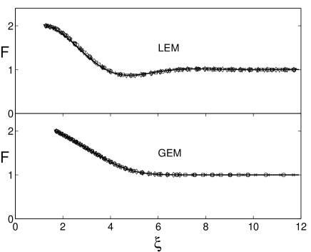
FIG. 2.: Solution of the reconstruction driven faceting scaling function in the LEM and GEM cases (solid lines) compared with scaled density functions from numerical simulations with $\epsilon=8$. Different symbols represent density functions at different times.

B Relaxation of an Infinite Bunch

In the second example we study the relaxation of an infinite bunch of steps. The initial step configuration (Fig. 1 (b)) consists of an infinite facet at $x<0$, in contact with an infinite array of uniformly spaced steps (at $x>0$). The first step has a single neighbor, and therefore its chemical potential is

$$\mu^{s}_{1}=\frac{-2g}{(x_{2}-x_{1})^{3}}\;.$$ (42)

In the LEM case there is a complication, since the first step may exchange adatoms with the infinite facet on its left. Hence we have to specify $\mu^{t}_{0}$, the adatom chemical potential on the facet. We assume here that $\mu^{t}_{0}=\mu^{s}_{1}$, neglecting any exchange of atoms between the first step and the facet. As a result the volume is conserved in the LEM case.

Simulations of this system in both the LEM and GEM cases suggest that the system exhibit scaling with the origin of the scaled position at the initial position of the first step. The leftmost steps from the bunch move to the left into the facet due to the repulsive interactions. The first step recedes in time and its position scales as $x_{1}\sim-t^{1/\gamma}$. At the same time the separation between the first steps grows. For $\xi<\xi_{1}$, the scaled position of the first step, the step density always vanishes, and we have to find the scaling function only for $\xi_{1}\leq\xi<\infty$.

1 Local Mass Exchange Mechanism

The velocity of the first step vanishes in the scaling limit. We can therefore evaluate $F(\xi_{1})$ by expanding $\dot{x}_{1}$ in $\theta^{-1}$, and requiring that the zeroth order term vanish. We find that the zeroth order term in $\dot{x}_{1}$ is proportional to $F^{3}(\xi_{1})$, which implies that $F(\xi_{1})=0$.

Two additional boundary conditions can be derived from the conservation of volume and the number of steps. Using Eqs. (24) and (29) to calculate changes in the volume and number of steps in the positive part of the $\xi$ axis together with equivalent equations for $\xi<0$, we find that

$$\left.\left[\xi\frac{d}{d\xi}\left(\frac{1}{F}\frac{d^{2}}{d\xi^{2}}\frac{3F^{2}}{2}\right)-\frac{1}{F}\frac{d^{2}}{d\xi^{2}}\frac{3F^{2}}{2}\right]\right|_{\xi_{1}}=0\;,$$ (43)

and

$$\left.\frac{d}{d\xi}\left(\frac{1}{F}\frac{d^{2}}{d\xi^{2}}\frac{3F^{2}}{2}\right)\right|_{\xi_{1}}=0\;.$$ (44)

As mentioned above, a zero of the scaling function is a singular point at which all derivatives of $F$ diverge. Since $F(\xi_{1})=0$, the limit $\xi\rightarrow\xi_{1}$ in the last two boundary conditions should be taken with care. This can be done by considering the power series (32). The differential equation (17) and the boundary conditions $F(\xi_{1})=0$, (43) and (44) impose connections between the coefficients of the expansion and leave only $b_{1}$ as a free parameter.

We now use the following procedure to compute $F$. For given values of $b_{1}$ and $\xi_{1}$ we approximate $F$ at $\xi_{1}+\delta\xi$ using the series expansion (32) with suitable truncation. At $\xi_{1}+\delta\xi$ the derivatives of $F$ are finite, and we solve $F$ from there by numerical integration. We adjust the values of $b_{1}$ and $\xi_{1}$ in order to satisfy the boundary condition at infinity, thus obtaining the scaling function $F(\xi)$ in the LEM case. In the upper half of Fig. 3 we compare this solution with simulation data.

2 Global Mass Exchange Mechanism

Since $\dot{x}_{1}\propto-(x_{2}-x_{1})^{-3}$, the requirement that the velocity of the first step vanishes in the scaling limit leads to the boundary condition

$$F(\xi_{1})=0\;.$$ (45)

To derive another boundary condition we use Eq. (31) and impose conservation of the number of steps. The following relation is thus obtained:

$$\left.\frac{dF^{3}}{d\xi}\right|_{\xi_{1}}=0\;.$$ (46)

This implies that all the coefficients in the series expansion (33) diverge except for $b_{1}$ which vanishes. Thus the convergence radius of (33) is zero and it is difficult to calculate the scaling function with the numerical procedure used in the LEM case. Nevertheless, taking a small enough value of $b_{1}$ and tuning $\xi_{1}$ to satisfy the boundary condition at infinity, we were able to calculate $F$ approximately. In the lower half of Fig. 3 we compare this approximation with simulation data.

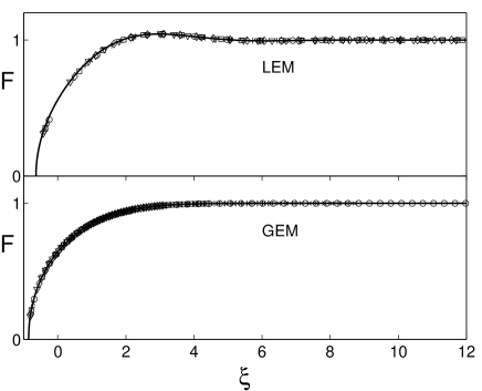
FIG. 3.: Solution of the infinite bunch scaling function in the LEM and GEM cases (solid lines) compared with scaled density functions from numerical simulations of the discrete model. Different symbols represent density functions at different times.

C Flattening Of A Groove

Our last example is the flattening of a groove cut in the crystal surface. The initial configuration (Fig. 1 (c)) consists of two infinite step bunches with steps of opposite signs that meet at the origin. Step repulsion within each bunch pushes the bottom step and anti-step towards each other until they collide and annihilate. We assume here that steps of opposite sign do not interact. Thus the chemical potential of the two bottom steps includes interaction with only one neighboring step, namely

$$\mu^{s}_{1}=\frac{-2g}{(x_{2}-x_{1})^{3}}\;.$$ (47)

When the first steps annihilate we relabel the remaining steps so that the positions of the bottom step and anti-step are always $x_{1}$ and $x_{0}$. Our system is symmetric with respect to the origin, and it is sufficient to consider only the positive part of the $x$ axis. Symmetry also excludes any flux of adatoms between the two bunches, and in the LEM case this implies that the volumes of the two bunches are conserved separately.

1 Local Mass Exchange Mechanism

The groove flattening problem is different from the two previous examples, where there was a well defined facet with its edge at the position of the first step. At the facet edge Eq. (17) becomes invalid due to the vanishing step density. In the groove example, steps annihilate at the origin, and there are steps in all regions of space. However, there could still be points where the density of steps vanishes if the position of the second step diverges in the scaling limit. Let us denote the scaled position of the facet edge by $\xi^{*}$. Eq. (17) is valid only for $\xi>\xi^{*}$, and the value of $\xi^{*}$ is unknown a priori. There are two possible, qualitatively different situations: 1) $\xi^{*}>0$, i.e., there is a plateau at the bottom of the groove which grow as $t^{1/4}$. 2) $\xi^{*}=0$. There could still be a diverging plateau, but it must grow more slowly than $t^{1/4}$. In what follows we rule out the first possibility and show that $\xi^{*}=0$.

According to Eq. (29), the number of step annihilation events grows with time as $t^{1/4}$. Denoting by $t_{n}$ the time of the $n$th annihilation event, we see that $t_{n}\sim n^{4}$ and $t_{n+1}-t_{n}\sim n^{3}$. We now show that if $\xi^{*}>0$, the time interval between annihilation events is larger than $n^{3}$. Just before the $n$th annihilation event, the velocity of the first step (which must be negative) is given by

$$\lim_{t\rightarrow t_{n}^{-}}\dot{x}_{1}=\frac{1}{4}\left(\frac{1}{(x_{3}-x_{2})^{3}}-\frac{2}{x_{2}^{3}}\right)\;.$$ (48)

If $\xi^{*}>0$, $x_{2}$ is of order $t_{n}^{1/4}\sim n$. Eq. (48) implies that $x_{3}-x_{2}>2^{-1/3}x_{2}$, and therefore the distance $x_{3}-x_{2}$ is also of order $n$.

After the $n$th annihilation event we relabel the steps. $x_{2}$ becomes $x_{1}$ , $x_{3}$ becomes $x_{2}$ and so on. Now the distance between the first two steps, $x_{2}-x_{1}$ is of order $n$. The velocity of the new first step, which is maximal (in absolute value) at this time, obeys the following inequality:

$$\lim_{t\rightarrow t_{n}^{+}}\left|\dot{x}_{1}\right|<\frac{1}{2(x_{2}-x_{1})^{3}}\sim{\cal O}\left(n^{-3}\right)\;.$$ (49)

The step must cross a distance of order $n$ until it annihilates and therefore $t_{n+1}-t_{n}$ is at least of order $n^{4}$, in contradiction with the relation $t_{n+1}-t_{n}\sim n^{3}$ derived above. Hence $\xi^{*}=0$.

In order to solve Eq. (17), we now find two boundary conditions at $\xi=0$. Consider first the quantity $x_{3}-x_{2}$. If $x_{2}$ diverges with time, $x_{3}-x_{2}$ must also diverge in order for $\dot{x}_{1}$ to be negative (see Eq. (48)). If $x_{2}$ does not diverge in the scaling limit, $x_{3}-x_{2}$ must still diverge in order for the time interval between two consecutive annihilation events to diverge in the scaling limit. Thus, $x_{3}-x_{2}$ diverges and the scaling function vanishes at the origin:

$$F(0)=0\;.$$ (50)

Another boundary condition is derived from volume conservation in the $x>0$ half of space. From Eq. (24) we obtain the condition

$$\left.\left[\xi\frac{d}{d\xi}\left(\frac{1}{F}\frac{d^{2}}{d\xi^{2}}\frac{3F^{2}}{2}\right)-\frac{1}{F}\frac{d^{2}}{d\xi^{2}}\frac{3F^{2}}{2}\right]\right|_{0}=0\;.$$ (51)

Requiring expansion (32) to satisfy Eqs. (17) and (51) we are left with two free expansion coefficients, which we tune in order to satisfy the boundary condition at infinity. The resulting solution compared to simulation data is shown in the upper half of Fig. 4.

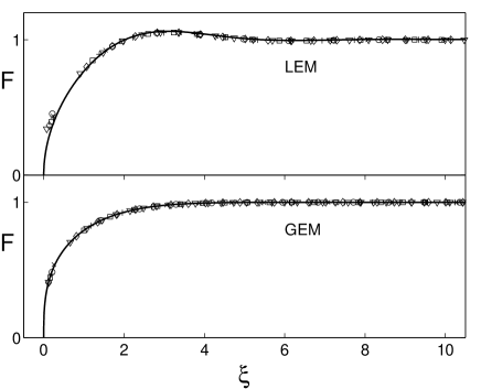
FIG. 4.: Solution of the groove flattening scaling function in the LEM and GEM cases (solid lines) compared with scaled density functions from numerical simulations of the discrete models. Different symbols represent density functions at different times.

2 Global Mass Exchange Mechanism

As in the LEM case, we have to find the value of $\xi^{*}$. From considerations similar to those used in the LEM case it can be shown that steps annihilate fast enough for scaling to occur only if $\xi^{*}=0$.

In the GEM case the volume is not conserved. However, by summing up the velocities of all the steps we can calculate the rate of change of the volume:

$$\frac{dV}{dt}=-\sum_{n=1}^{\infty}\dot{x}_{n}=\frac{1}{2}\lim_{N\rightarrow\infty}\frac{1}{(x_{N}-x_{N-1})^{3}}\;.$$ (52)

The r.h.s. of Eq. (52) is $F_{\infty}^{3}/2$, while the l.h.s. can be calculated from Eq. (26) with $\xi_{a}=0$, $\xi_{b}=\infty$ and $\theta^{2}=t$. This calculation combined with Eq. (52) leads to the boundary condition

$$\left.\left(F^{3}-3\xi F^{2}F^{\prime}\right)\right|_{0}^{\infty}=F_{\infty}^{3}\;,$$ (53)

which implies

$$F(0)=0.$$ (54)

To calculate the scaling function we use the series expansion (33) to approximate $F$ near the singular point and then integrate Eq. (18) numerically from a point where $F$ is finite. We tune the expansion coefficient $b_{1}$ to satisfy the boundary condition at infinity. The resulting solution compared to simulation data is shown in the lower half of Fig. 4.

VI Summary and Discussion

We studied 1D step-flow models for the kinetics of faceting and relaxation and showed that the surface profile exhibits scaling behavior. The value of the scaling exponents was determined by the mass transport mechanism. The scaling functions in all cases considered here were described by the same differential equation for the same mass transport mode. These scaling functions differ from those predicted by Mullins’ continuum theory, which does not explicitly consider the existence of steps. However, the scaling exponents $\gamma$ agree with Mullins’ classical theory. This can be understood as follows. The systems considered here are well below the roughening temperature of the (low-index) singular surface but large parts of the system are rough, with nonzero macroscopic slope and a differentiable free energy as a function of orientation. Therefore, if the system shows scaling behavior at all, the whole system (including the singular region) must evolve with the same time dependence as the non-singular part, which is accurately described by Mullins’ model.

Here we only considered attachment/detachment limited kinetics for local mass exchange. We have carried out a similar scaling analysis for diffusion limited kinetics. Diffusion limited kinetics is also a local mass exchange mode and hence the scaling exponents are the same as for attachment/detachment limited kinetics. However, the differential equation for the diffusion limited scaling function is different from the attachment/detachment limited case. For diffusion limited kinetics we found equations, which under the scaling assumption, are equivalent to the continuum models proposed in Refs. [7, 15]. Our results are valid even for finite step permeability at sufficiently long times.

Another issue that we would like to investigate further is the condition for scaling behavior. When a step profile shows a scaling behavior, the scaling exponent should depend on the mass transport mechanism but not the driving force of the evolution at the boundary. However, very strong driving forces could cause a piling up of steps and destroy the scaling behavior. What kind of driving force gives rise to a scaling behavior? For example, for the flattening of a groove, we used a contact interaction between steps with opposite signs. What kind of interaction between the steps of opposite signs in the middle, in general, results in a profile that obeys scaling? Does it depend on the mass transport mechanism? We have examined some artificial examples (not described here) of interactions between the steps of opposite signs that can destroy the scaling behavior but do not know yet the general form of the driving forces that admit a scaling ansatz.

One can also consider more general interactions between neighboring steps in the non-singular region. Although our scaling analysis is valid for a general step-step interaction (see Appendix A), we only carried out simulations to verify that scaling indeed occurs in the case of simple entropic and elastic step-step interactions. What are the interactions that support scaling? What is the general relationship between the boundary conditions and the step interactions that is consistent with a scaling ansatz? If these questions can be answered, we may be able to tell in advance which surface systems will show dynamic scaling behavior.

We are grateful to Da-Jiang Liu for helpful discussions. This work was supported in part by grant No. 95-00268 from the United States-Israel Binational Science Foundation (BSF), Jerusalem, Israel, by the Korea Research Foundation, Grant D00001, and by the National Science Foundation (NSF-MRSEC grant #DMR96-32521).

A

In this appendix we give the results of a scaling analysis with a general step chemical potential formula. We start by replacing Eq. (3) with

$$\mu_{n}^{s}=U\left(x_{n}-x_{n-1}\right)-U\left(x_{n+1}-x_{n}\right)\;,$$ (A1)

with $U(x)$ a general analytic function of $x$. Such a formula is consistent with interactions between nearest neighbor steps.

Next we use this formula together with the step velocities (5) and (7) to rewrite Eq. (11) in the LEM and GEM cases. Changing the step velocities does not alter the expansion (15) since this expression is general and depends only on the scaling function $F$. We can thus use expansion (15) to expand the new Eq. (11) in powers of $\theta^{-1}$. We find that in the LEM case

$$\theta {}^{\gamma-4}\frac{a^{2}k}{2}\frac{d^{2}}{d\xi^{2}}\left[\frac{1}{F}\frac{d}{d\xi}\left(\frac{1}{F}\frac{dU\left(\frac{1}{F}\right)}{d\xi}\right)\right]$$ (A2)

$$- \frac{\xi}{\gamma}\frac{dF}{d\xi}+{\cal O}\left(\theta^{\gamma-6}\right)=0\;.$$ (A3)

This implies that in the LEM case $\gamma=4$ and the differential equation for the scaling function is

$$2a^{2}k\frac{d^{2}}{d\xi^{2}}\left[\frac{1}{F}\frac{d}{d\xi}\left(\frac{1}{F}\frac{dU\left(\frac{1}{F}\right)}{d\xi}\right)\right]-\xi\frac{dF}{d\xi}=0\;.$$ (A4)

In the GEM we find that

$$\theta^{\gamma-2}a^{2}k\frac{d^{2}U\left(\frac{1}{F}\right)}{d\xi^{2}}+\frac{\xi}{\gamma}\frac{dF}{d\xi}+{\cal O}\left(\theta^{\gamma-4}\right)=0\;,$$ (A5)

which implies $\gamma=2$ and

$$2a^{2}k\frac{d^{2}U\left(\frac{1}{F}\right)}{d\xi^{2}}+\xi\frac{dF}{d\xi}=0\;.$$ (A6)

REFERENCES

- [1] For general reviews see H.-C. Jeong and E. D. Williams, Surf. Sci. Rep. 34, 171 (1999); E. D. Williams, Surf. Sci. 299/300, 502 (1994).
- [2] W. W. Mullins, Phil. Mag. 6, 1313 (1961). See also W. W. Mullins, J. Appl. Phys. 28, 333 (1957).
- [3] W. K. Burton, N. Cabrera and F. C. Frank, Philos. Trans. R. Soc. London, Ser. A 243, 299 (1951).
- [4] In the more general case of a finite ratio between the terrace diffusion rate and the step-edge attachment rate, varies with position and must be calculated explicitly by solving the diffusion equation. This does not change our basic conclusions.
- [5] V. I. Marchenko and A. Ya. Parshin, Zh. Eksp. Teor. Fiz. 79, 257 (1980) (Sov. Phys. JETP 52(1), 129 (1980)).
- [6] A. F. Andreev and Yu. A. Kosevich, Zh. Eksp. Teor. Fiz. 81, 1435 (1981) (Sov. Phys. JETP 54(4), 761 (1982)).
- [7] M. Ozdemir and A. Zangwill, Phys. Rev. B 42, 5013 (1990).
- [8] A. Rettori and J. Villain, J. Phys. France 49, 257 (1988).
- [9] H.-C. Jeong and J. D. Weeks, Scann. Micro. (in press).
- [10] N. Israeli and D. Kandel, Phys. Rev. Lett. 80, 3300 (1998).
- [11] N. Israeli and D. Kandel, Phys. Rev. B. 60, 5946 (1999).
- [12] D.-J. Liu, E. S. Fu, M. D. Johnson, J. D. Weeks and E. D. Williams, J. Vac. Sci. Technol. B. 14, 2799 (1996).
- [13] P. Nozières, J. Phys. I France 48, 1605 (1987).
- [14] H.-C. Jeong and J. D. Weeks, Phys. Rev. Lett. 75, 4456 (1995).
- [15] J. Hager and H. Spohn, Surf. Sci. 324, 365 (1995).