Particle Dynamics in a Mass-Conserving Coalescence Process

Abstract

We consider a fully asymmetric one-dimensional diffusion model with mass-conserving coalescence. Particles of unit mass enter at one edge of the chain and coalesce while performing a biased random walk towards the other edge where they exit. The conserved particle mass acts as a passive scalar in the reaction process $A+A\rightarrow A$, and allows an exact mapping to a restricted ballistic surface deposition model for which exact results exist. In particular, the mass-mass correlation function is exactly known. These results complement earlier exact results for the $A+A\rightarrow A$ process without mass. We introduce a comprehensive scaling theory for this process. The exact analytical and numerical results confirm its validity.

Diffusion-limited chemical processes are at the focus of recent research. These are dynamic systems where the chemical reaction time scales are short compared to those controlling spatial fluctuations in concentration. The latter dominate the kinetics, in particular in low dimensions. Such processes display dynamic scale invariance with scaling properties that are robust, tend to be universal, and not sensitive to many details of the actual dynamics at the microscopic level. Simplified models are therefore able to catch the essence of the process. Moreover, some of these models are accessible to exact solutions in one dimension.

An example of these is the one-species coalescence process, $A+A\rightarrow A$ [1, 2, 3, 4, 5]. Exact results for this process were obtained recently using the so-called inter-particle distribution function (IPDF) method, also known as the method of empty intervals [6]. This includes several versions of the model, with and without external input of particles and in the presence or absence of a diffusion bias along the chain [7, 8]. In this letter we address the fully asymmetric diffusion case where particles enter at one edge of the chain, and coalesce when they meet each other, while performing a driven random walk towards the other edge [8]. We enhance this model by assigning a mass to each particle, which is preserved during each merging event.

Consider a linear chain with $L$ sites. Particles of unit mass enter at the left boundary $x=1$, diffuse to the right and coalesce when they meet, and ultimately exit at the right boundary $x=L$. The diffusion of the particles along the chain is totally biased. Choose a site $x$ at random. If occupied, the particle at this site moves to the next site $x\to x+1$. If site $x+1$ is already occupied, the two particles merge,

$$m_{x}(t+1)=0~{}~{}{\rm and}~{}~{}m_{x+1}(t+1)=m_{x+1}(t)+m_{x}(t)$$ (1)

with $m$ the total mass of each particle. Total mass is conserved during coalescence. Site $x=1$ is the input boundary. If chosen as an update site, it is immediately refilled by the reservoir $m_{1}(t+1)=1$ and $m_{2}(t+1)=m_{2}(t)+m_{1}(t)$ At the opposite edge, $x=L$, the particles simply fall off the chain, $m_{L}(t+1)=0$, back into the reservoir.

The mass rides like a passive scalar on top of the particles. It has no effect on the transition probabilities. We could describe the process just as well in terms of only occupation numbers, $c_{x}=0,1,$ for empty or occupied site. The latter is the fully asymmetric $A+A\rightarrow A$ process.

The mass is a useful parameter. It allows an exact mapping onto an exactly soluble restricted ballistic surface deposition (RBD) model [9]. Consider a one dimensional interface, as shown in Fig.1. The steps in the downward staircase can take any magnitude $m_{x}=0,1,2,\cdots$. During each time step, one of the columns at $x+\frac{1}{2}$ is chosen at random, $m_{x}$ particles are deposited onto it such that the entire step fills up and the step at $x+1$ grows to $m_{x+1}+m_{x}$. Exact results for this RBD model have been obtained earlier using a generating function approach [9]. We can reinterpret those exact results in framework of the asymmetric $A+A\rightarrow A$ reaction process.

Starting from the master equation, closed form recursive equations of motion are obtained for the mass distribution along the chain $M(x,t)=\langle m_{x}(t)\rangle$ and also (as discussed later) the two-point mass correlations. $M(x,t)$ obeys the relation

$$M(x,t+1)=(1-\frac{1}{L})M(x,t)+\frac{1}{L}M(x-1,t)$$ (2)

with boundary condition $M(1,t)=1$ (see eqs.(8)-(15) in reference [9] for details). This implies that in the stationary state the mass distribution is uniform, $M(x)=1$, and there is a direct link between particle concentration $C(x)=\langle c_{x}\rangle$ and the average mass carried by each particle, $\tilde{M}(x)$. They are exactly related as $\tilde{M}(x)=M(x)/C(x)$ where $\tilde{M}(x)$ measures the average mass over occupied sites only. Particle coalescence creates increasingly heavier particles in the chain towards the right. At the same time they become more sparsely spaced, because on average the mass remains constant along the chain.

In the alternate RBD surface representation, this means that although the step heights increase along the surface from left to right, the steps occur at correspondingly larger intervals, such that the stationary state average slope of the staircase remains constant.

This dynamic process has a peculiar hierarchical structure. Consider the path of one unit of mass. It performs a biased random walk, but completely uncorrelated from all other masses. Similarly, two specific mass units perform completely independent random walks, until the moment they meet. From there on they move randomly but as a bound pair. Again, all other particles play no role.

This hierarchical property suggests the following scaling theory. Consider a specific unit of mass. It moves to the right with average velocity $v=1$. The standard deviation in its position is proportional to the square root of the time and distance traveled, i.e. $\Delta r\sim x^{\frac{1}{2}}$. While diffusing to the right this particle merges with other masses. The total amount of mass it sweeps up is expected then to be of order $\Delta r$, i.e., that the average mass of occupied sites scales as $\tilde{M}(x)\sim x^{\frac{1}{2}}$. The amount of swept-up mass does not depend on the particle concentration $C(x)$, because although the merging events reduce in frequent, they increase in size. However, this increasing lumpiness will show in increasing statistical fluctuations along the chain in Monte Carlo simulations.

Next, we predict that the above random walk exponents are exact. This presumes the absence of intricate correlations between the particles. The hierarchical structure of the equations of motion, and the diffusion equation structure of recursion relations in both exact solution methods suggest this prediction. In the following we demonstrate the validity of this scaling theory from both numerical and analytical exact results.

Hinrichsen et al.[8] obtained the exact stationary state particle concentration. It scales as

$$C(x)=\sqrt{\frac{1}{\pi x}}[1+\frac{3}{8x}]+O(x^{-5/2}).$$ (3)

This agrees with our scaling theory, because of the exact relation $\tilde{M}(x)=M(x)/C(x)$. The scaling argument predicts that $\tilde{M}(x)$ grows as $x^{\frac{1}{2}}$, while eq.(2) implies that $M(x)=1$.

Figure 2 illustrates the above numerically. It shows the time evolution of the particle density at various values of $x$ starting from the uniform initial state where every site is occupied by one unit of mass particle. We averaged over 10 independent Monte Carlo runs. Initially the curves coincide, until the time when particles from the input edge reach that specific site. As expected this crossover time scales linearly with $x$, i.e., with the uniform average particle velocity along the chain. The slope of the initial curve is $C(x,t)\sim t^{-\frac{1}{2}}$, and the stationary state plateau values scale as $C(x)\sim x^{-\frac{1}{2}}$, both in accordance with the scaling theory. Notice also that the statistical fluctuations increase with the distance from the source $x$.

The mass auto-correlation function, $w_{m}^{2}=\langle m_{x}^{2}\rangle-\langle m_{x}\rangle^{2}$ measures these fluctuations, and is a special case of the two-point correlator discussed below for which we have an exact solution from the mapping to the RBD model. At large $x$ the fluctuations grow as $w_{m}(x)\simeq\sqrt{x}$, in accordance with our random-walk based scaling theory. We checked numerically the fluctuations in the particle density. Fig.3 shows that they decay as $w_{p}\simeq A/\sqrt{x}$, again consistent with the scaling theory.

Consider the particle-particle correlation function, $g_{p}(x,r)=\langle c_{x}c_{x+r}\rangle-\langle c_{x}\rangle\langle c_{x+r}\rangle$ and the mass-mass correlation function, $g_{m}(x,r)=\langle m_{x}m_{x+r}\rangle-\langle m_{x}\rangle\langle m_{x+r}\rangle$. As far as we know, no exact results are available for $g_{p}(x,r)$, from the method of empty intervals, although it seems within reach. On the other hand, the two-point mass correlator $G_{m}(x,y,t)=\langle m_{x}(t)m_{y}(t)\rangle$ was shown in [9] to obey in the stationary steady state the recursion relations

$$G_{m}(1,x) =G_{m}(1,x-1),$$ (4)

$$G_{m}(x,x) =2G_{m}(x-1,x)+G_{m}(x-1,x-1),$$ (5)

$$G_{m}(x-1,x) =\frac{1}{2}G_{m}(x-2,x),$$ (6)

$$G_{m}(x,y) =\frac{1}{2}[G_{m}(x-1,y)+G_{m}(x,y-1)],$$ (7)

where $|x-y|\geq 2$. This set of coupled equations can be solved exactly,

$$G_{m}(1,x) =1,$$ (8)

$$G_{m}(x,x) =1+4(x-1)Z_{2(x-1)}(0),$$ (9)

$$G_{m}(x-1,x) =Z_{2(x-2)}(0),$$ (10)

$$G_{m}(x,y) =\sum_{n=0}^{r-1}Z_{2(y-2)}(n)=1-\sum_{n=r}^{y-2}Z_{2(y-2)}(n),$$ (11)

with $r\equiv(y-x)>0$, and

$$Z_{2p}(n)=\frac{(2p-n)!}{p!(p-n)!}(\frac{1}{2})^{2p-n},$$ (12)

which is related to the probability that a random walker returns to its starting point exactly $n$ times up to $2p$ steps, see [9] for details.

We expect the following scaling form for both $g_{m}$ and $g_{p}$ in the stationary state:

$$g_{\alpha}(x,r)=b^{-2{\rm x}_{\alpha}}g_{\alpha}(b^{-1}x,b^{-1/2}r),$$ (13)

with $b$ an arbitrary scale factor. The distance $r$ from the source plays the role of time in our diffusion-coalescence type scaling argument. Therefore $r$ should scale with respect to the correlator distance $x$ as $r\sim\sqrt{x}$. The other exponents, ${\rm x}_{p}$ and ${\rm x}_{m}$, follow by power-counting. They must be the dimensions of the particle and mass concentrations, $C(x)$ and $M(x)$, which are equal to ${\rm x}_{p}=\frac{1}{2}$ and ${\rm x}_{m}=0$ according to the previous discussion. We perform numerical simulations for $g_{p}$, and exact enumerations of the exact formula for $g_{m}$. Fig.4 and Fig.5 show the scaling functions $f_{p}$ and $f_{m}$, defined as

$$g_{p}=x^{-1}f_{p}(r/\sqrt{x}),$$ (14)

$$g_{m}=f_{m}(r/\sqrt{x}),$$ (15)

The data collapses perfectly and thus confirms the validity of the scaling relations, eq.(13).

Both scaling functions vanish at large $R=r/\sqrt{x}$, as they should. At small $R$ they are both linear in the scaling variable. It is easy to evaluate the exact recursion relations for $G_{m}$ in the limit of large $x$ and fixed small $r$. This yields $f_{m}(R)\simeq-1+\frac{1}{\sqrt{\pi}}R$.

The particle correlator scaling function is also linear at small $R$. We find numerically that

$$f_{p}(R)\simeq-a+bR$$ (16)

with $a=0.318(1)$ and $b=0.268(6)$ and we suspect that the overall factor $a=1/\pi$.

The above numerical and exact results are all in full agreement with the simple scaling picture where we treat the particles as performing free independent biased random walks before they merge. None of the scaling exponents differ from their diffusion values. The final verification for the validity of this intuitive explanation is the shape of the stationary state mass distribution function, $p(m,x)$, i.e., the probability to find a particle of mass $m$ at a site $x\gg 1$. Our scaling theory presumes that this distribution behaves in the same manner as the probability for a specific tagged particle to reach site $x$ with mass $m$. Each tagged particle follows an independent biased random walk and its mass grows proportional to the spatial fluctuations about its average path.

Fig.6 shows numerical results for $p(m,x)$ at system size $L$=512 for various values of $x$=16, 64, 256, and 512. It is obtained from 10 independent runs, each $10^{6}$ Monte Carlo steps long. The data is plotted in terms of $\sqrt{x}p(m,x)$ versus the scaling variable $\xi=m/\sqrt{\pi x}$ and collapses well onto Gaussian with a linear prefactor,

$$p(m,x)=A~{}\frac{m}{x}~{}\exp(-Bm^{2}/x).$$ (17)

The parameters $A$ and $B$ are predetermined by the normalization condition and the scaling of the particle density (see eq.(3))

$$\sum_{m=0}^{\infty}p(m,x)=1,$$ (18)

$$\tilde{M}(x)=\sum_{m=0}^{\infty}mp(m,x)=1/C(x),$$ (19)

which yields $A=\frac{1}{2}$ and $B=\frac{1}{4}$. The drawn curve in Fig.6 corresponds to this Gaussian with the above values of $A$ and $B$. Eq.(17) is the simplest Gaussian form consistent with the requirement that $p(m,x)$ vanishes in the limit $m\to 0$. According to our intuitive picture, $p(m,x)$ is related to the probability that a biased random walker with drift velocity $v_{d}=\frac{1}{2}$, makes an excursion of size $m$ from its average path before reaching site $x$, irrespective of (i.e., averaged over all) the starting times at site $x=1$.

In conclusion, we present new exact results for the $A+A\rightarrow A$ type coalescense process by introducing mass to the particles, and exploring the exact mapping to a surface deposition model, the so-called RBD type surface growth model. In addition, we propose a scaling theory based on the assumption we can treat the particles as performing free independent biased random walks before they merge. All scaling exponents should then take naive diffusion values. The above numerical and exact results are all in full agreement with this random walk type scaling. It appears therefore that the scaling properties of $A+A\rightarrow A$ type dynamics are now fully understood, and actually, in the final analysis, are predictable from random walk considerations only.

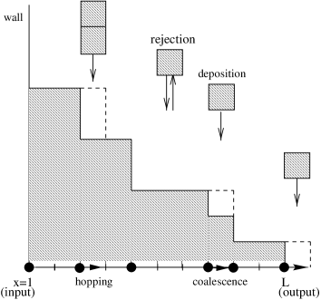
FIG. 1.: Surface representation of the $A+A\rightarrow A$ process. The step heights along the stairway represent the mass of the particles. Each deposition process fills-up the entire step, such that the adjacent step has a new height equal to the sum of the two.

FIG. 2.: The time dependent particle concentration $\langle c(x)\rangle$ as function of time at various values of the distance from the source, $x=16(\times),32(\circ),64(\bullet),128(\bigtriangleup),256(\bigtriangledown)$, and $512(\diamond)$ at chain length $L=512$. The slope of the drawn line is -1/2.

FIG. 3.: fluctuations in the particle concentration from the auto-correlation functions $w_{p}^{2}(x)=\langle c^{2}(x)\rangle-\langle c(x)\rangle^{2}$ at chain length $L=512$. The slope of the drawn line is -1/2.

FIG. 4.: The scaling function for the particle-particle correlator $g_{p}$, from 10 independent Monte Carlo runs each averaged over $10^{6}$ time steps at chain length $L=512$ for various distances from the source, $r=1(+),2(\times),4(\circ),8(\bigtriangleup),16(\bigtriangledown)$, and $32(\diamond)$. The drawn line is obtained from eq.(16).

FIG. 5.: The scaling function of the mass-mass correlator $g_{m}$, from enumeration of the exact recurrence relations, at chain length $L=512$ for various distances from the source, $r=2(\times),4(\circ),8(\bigtriangleup),16(\bigtriangledown)$, and $32(\diamond)$. The drawn line is the tangent at small $R$, see between eq.(14) and eq.(16).

FIG. 6.: Numerical Monte Carlo scaling plot of the stationary state distribution $p(m,x)$, the probability to find a particle of mass $m$ at site $x$, for various $x=16(\times),64(\circ),256(\bullet)$, and $512(\triangle)$. We plot $\sqrt{x}p(x,m)$ versus $\xi=m/\sqrt{\pi x}$, the Gaussian form of eq.(17).

REFERENCES

- [1] M. Bramson, and D. Griffeath, Ann. Prob. 8, 183 (1980); Z. Wahrsch. Geb. 53 183 (1980).
- [2] D. C. Torney and H. M. McConnell, Proc. Roy. Soc. Lond. A 387, 147 (1983); L. Peliti, J. Phys. A19, L365 (1985); Z. Rácz, Phys. Rev. Lett. 55 1707 (1985).
- [3] A. A. Lushnikov, Phys. Lett. A 120, 135 (1987); J. L. Spouge, Phys. Rev. Lett. 60, 871 (1988).
- [4] V. Privman, J. Stat. Phys. 69. 629 (1992); J. Stat. Phys. 72, 845 (1993); E. Clément, R. Kopelman, and L. Sander, Chem. Phys. 180 337 (1994).
- [5] M. A. Burschka, C. R. Doering, and D. ben-Avraham, Phys. Rev. Lett. 63, 700 (1989); D. ben-Avraham, M. A. Burschka, and C. R. Doering, J. Stat. Phys. 60, 695 (1990); C. R. Doering, M. A. Burschka, and W. Horsthemke, J. Stat. Phys. 65, 953 (1991); C. R. Doering, Physica A 188, 386 (1992); D. ben-Avraham, Mod. Phys. Lett. B 9, 895 (1995).
- [6] C. R. Doering and D. ben-Avraham, Phys. Rev. A 38, 3035 (1988); C. R. Doering, and M. A. Burschka, Phys. Rev. Lett. 64 245 (1990).
- [7] Z. Cheng, S. Redner, and F. Leyvraz, Phys. Rev. Lett. 62, 2321 (1989).
- [8] H. Hinrichsen, V. Rittenberg, and H. Simon, J. Stat. Phys. 86, 1203 (1997).
- [9] H. Park, M. Ha, and I. Kim, Phys. Rev. E 51, 1047 (1995).
- [10] D. ben-Avraham, in Nonequilibrium Statistical Mechanics in One Dimension, edited by V. Privman (Cambridge University Press, Cambridge, United Kingdom, 1997).