Thermal vortex dynamics in a two-dimensional condensate

Abstract

We carry out an analytical and numerical study of the motion of an isolated vortex in thermal equilibrium, the vortex being defined as the point singularity of a complex scalar field $\psi({\bf r},t)$ obeying a nonlinear stochastic Schrödinger equation. Because hydrodynamic fluctuations are included in this description, the dynamical picture of the vortex emerges as that of both a massive particle in contact with a heat bath, and as a passive scalar advected to a background random flow. We show that the vortex does not execute a simple random walk and that the probability distribution of vortex flights has non-Gaussian (exponential) tails.

05.70.Fh, 11.27.+d, 74.20.De

I Introduction

Vortices and other topological field configurations play a fundamental role in determining the properties of many fascinating materials and control the physical mechanisms underlying several applications. Examples include superfluids [2], superconductors [3, 4], periodic solids [5], liquid crystals [6], two-dimensional magnets [7], propagating coherent light beams [8], and perhaps even the hot plasma that filled the very early Universe [9]. Common aspects of the phenomenology of these diverse applications stem from the mathematical similarity of the underlying field theories and their classical static solutions.

Models of vortices as Brownian point particles, characterized by a mass, mutual interactions, and damping, are commonly used to study the behavior of superconductors and superfluids [10]. In this picture the equation of motion for a single overdamped vortex, not subject to any external forces, is extremely simple:

$$\gamma\dot{\bf r}(t) = {\bf f}(t);$$ (1)

$$\langle f_{\mu}(t)f_{\nu}(t^{\prime})\rangle = \frac{2\gamma k_{B}T}{M}\delta_{\mu,\nu}\delta(t-t^{\prime}),$$ (2)

where $\gamma$ is the damping coefficient, $M$ is the vortex mass, ${\bf f}(t)$ is a Gaussian thermal noise, $\mu,\nu\in\{x,y\}$, and $\langle\cdots\rangle$ denotes canonical ensemble averaging. It follows that the vortex velocity distribution is also Gaussian.

This effective picture is extremely appealing—primarily because of the drastic reduction of the number of degrees of freedom. However, to our knowledge, it has not been shown to be derivable from the dynamics of an underlying field theory. In this paper we study this question by solving both analytically and numerically for the motion of the vortex as an effective degree of freedom arising in a stochastic nonlinear Schrödinger equation. It is well-known that the conventional description of Brownian motion in terms of equations such as (2), that of a heavy particle interacting with light scatterers, ignores the presence of hydrodynamic fluctuations. A more complete description would allow us not only to test the validity of the Brownian motion model for the vortex but also to compute corrections to it and, possibly, to find new physical effects.

Our analytic approach rests on the use of a singular perturbation expansion around a rigid vortex utilizing a low-temperature or weak-noise expansion. We are able to derive a Fokker-Planck equation for the single vortex distribution function which corresponds to that of a passive scalar advected to a background flow [not just a simple diffusion equation as would be predicted by Eqs. (2)]. In our numerical work we are able to extract the diffusion constant for the vortex motion which turns out to be in good agreement with the theoretical prediction. Consistent with our theoretical analysis, the vortex effective mass diverges logarithmically with the system size. We also investigate the statistics of vortex flights and demonstrate that the probability distribution function (PDF) has an exponential tail implying nontrivial correlations in the background thermal flow field.

In Section I we present the stochastic nonlinear Schrödinger equation and discuss its physical relevance. In Section II we use the low-temperature perturbative expansion about the vortex collective coordinates to derive its equation of motion. Section III describes our numerical techniques and the associated results. We end with Section IV with a further discussion of our conclusions.

II The Stochastic Nonlinear Schrödinger Equation

We study the motion of an isolated vortex by considering it as a singularity of a classical stochastic nonlinear Schrödinger field $\psi({\bf r},t)$ in two spatial dimensions. The equation of motion of this model theory is $(a<0)$:

$$(i\hbar-\gamma)\frac{\partial\psi}{\partial t} = -\frac{\hbar^{2}}{2m}\nabla^{2}\psi+a\psi+b|\psi|^{2}\psi+\eta({\bf r},t);$$ (3)

$$\langle\eta({\bf r},t)\eta^{*}({\bf r}^{\prime},t^{\prime})\rangle = 2k_{B}T\gamma\delta(t-t^{\prime})\delta({\bf r}-{\bf r}^{\prime}),$$ (4)

$$\langle\eta({\bf r},t)\eta({\bf r}^{\prime},t^{\prime})\rangle = 0.$$ (5)

The damping coefficient $\gamma$ and the stochastic force $\eta({\bf r},t)$ model the coupling of the condensate to a heat bath, satisfying the fluctuation-dissipation relation. Coefficients $a$, $b$ and $m$ are assumed constant and independent of temperature; thermal effects are fully described by the stochastic force.

The above equations (5) describe the phenomenology of physically important systems such as atomic Bose condensates [11] and superfluid helium II [12, 13]. The same equation (at $T=0$), amended as appropriate by the vector potential, describes the order-parameter dynamics of type-II superconductors [14, 15]. Although the above is known to be strictly true only for a class of type-II superconductors with magnetic impurities [16], it is often assumed that Eqs. (5) apply to all type-II superconductors, unless indicated otherwise. We will henceforth study these equations as an important paradigmatic field theory representing a broad range of related physical phenomena.

It is convenient to make all quantities dimensionless by standard substitutions. We set $\psi=\tilde{\psi}\sqrt{-a/b}$, $\gamma=\tilde{\gamma}\hbar$, $t=\tilde{t}\gamma/(-a)$, ${\bf r}=\tilde{\bf r}\hbar/\sqrt{-2am}$, $\eta=\tilde{\eta}(-a)\sqrt{-a/b}$, and $k_{B}T=-a\hbar^{2}/(2\tilde{\beta}mb)$. Note that ${\bf r}$ is normalized to a unit of length $\hbar/\sqrt{-2am}$, which is the Ginzburg-Landau coherence length, usually denoted $\xi$. With these substitutions, and after dropping the tildes, Eqs. (5) become

$$(i/\gamma-1)\frac{\partial}{\partial t}\psi = -\nabla^{2}\psi+[|\psi|^{2}-1]\psi+\epsilon\eta({\bf r},t);$$ (6)

$$\langle\eta({\bf r},t)\eta^{*}({\bf r}^{\prime},t^{\prime})\rangle = \frac{2}{\beta}\delta(t-t^{\prime})\delta({\bf r}-{\bf r}^{\prime}),$$ (7)

$$\langle\eta({\bf r},t)\eta({\bf r}^{\prime},t^{\prime})\rangle = 0.$$ (8)

The position of an isolated vortex, ${\bf R}(t)$, is defined via a contour integral

$$\oint[\nabla\mbox{arg}\,\psi({\bf r},t)]\cdot d\,{\bf l},$$ (9)

which equals $2\pi$ when the integration path encloses the point ${\bf R}(t)$, and vanishes otherwise.

The Brownian motion of vortices as point particles has been argued to hold primarily in the overdamped limit ($\gamma\rightarrow\infty$), which is directly relevant to the superconducting case; this is also the limit studied in this paper. We envision a situation in which a single vortex exists in the ground state of the field $\psi({\bf r},t)$. In a thin superconducting film one can in principle achieve the same effect by placing the sample in a magnetic field of one flux quantum per sample area. In the latter case there are many other factors of practical importance, such as geometrical and point pinning, which however will not be dealt with here. The vortex is assumed to be located near the center of the spatial extent of the condensate, so that boundary effects can be neglected. The radius of the sample $\Lambda_{c}$ provides a natural infrared cutoff. At sufficiently low temperature, thermally induced vortex-antivortex pairs will be exponentially suppressed and we may assume that there is only one vortex in a spatially bounded superfluid film at all times. This assumption has been verified numerically for a range of temperatures and sample sizes studied.

III Perturbative Analysis of Vortex Transport

In this Section we utilize the singular perturbation expansion of Kaup [17] to extract the vortex position from the stochastic equation of motion (8). We first expand the field as

$$\psi({\bf r},t) = \psi_{0}({\bf X})+\epsilon\phi({\bf r},t);$$ (10)

$$\phi({\bf r},t) = \phi_{1}({\bf X},t)+\epsilon\phi_{2}({\bf X},t)+\cdots,$$ (11)

where ${\bf X}\equiv(X,Y)$ is the comoving coordinate, measured relative to a moving reference point; ${\bf X}(t)={\bf r}-{\bf R}^{0}(t)$. The absence of explicit time dependence in $\psi_{0}({\bf X})$ in the comoving reference frame indicates that it is the static vortex field in the absence of fluctuations. Tomboulis [18] has shown that introduction of a collective coordinate such as ${\bf R}^{0}(t)$, while conserving the total number of dynamical degrees of freedom, is a canonical transformation. The fluctuating field $\phi({\bf r},t)$ can be thought of as a superposition of harmonic modes in the background of the rigid vortex $\psi_{0}({\bf X})$. The phonons are gapless [19], therefore they will be an important consideration at any finite temperature. The variable $\epsilon\ll 1$ plays the role of a small parameter as well as that of a bookkeeping device to control the perturbation series [20]. Another useful way to think about $\epsilon$ emerges when one absorbs $\epsilon$ into the definition of $\eta({\bf r},t)$ in Eq. (8): $\epsilon$ then reappears as the square root of temperature in the fluctuation-dissipation relation in Eqs. (8). Therefore, the small-$\epsilon$ expansion is actually the small temperature or weak noise expansion. The equation of motion (8) is required to hold at every order in $\epsilon$, which results in a hierarchy of equations for $\psi_{0}({\bf X})$, $\phi_{1}({\bf X},t)$, etc.

Because of the added fluctuations in Eq. (10), the actual vortex position ${\bf R}(t)$ as the singularity of the full dynamical field $\psi({\bf r},t)$ does not in general coincide with the coordinate ${\bf R}^{0}(t)$, which by definition is the singularity of the rigidly moving static vortex field $\psi_{0}({\bf X})$. The two are related via

$${\bf R}(t)=\vec{\rho}\,[{\bf R}^{0}(t),\epsilon\phi]={\bf R}^{0}(t)+\epsilon\int d^{2}{\bf r}\left.\frac{\delta\vec{\rho}\,[{\bf R}^{0}(t),\phi]}{\delta\phi({\bf r})}\right|_{\phi=0}\phi({\bf r},t)+\mbox{c.c.}+\cdots,$$ (12)

where $\vec{\rho}\,[{\bf R}^{0}(t),\epsilon\phi]$ is a vector functional of the fluctuation field $\epsilon\phi({\bf r},t)$ and of the reference point ${\bf R}^{0}(t)$. We define

$$\dot{{\bf R}}^{0}(t) = 0+\epsilon{\bf v}^{0}_{1}(t)+\epsilon^{2}{\bf v}^{0}_{2}(t)+\cdots,$$ (13)

$$\dot{{\bf R}}(t) = 0+\epsilon{\bf v}_{1}(t)+\epsilon^{2}{\bf v}_{2}(t)+\cdots,$$ (14)

which makes explicit the fact that there is no vortex motion in the absence of thermal fluctuations. Differentiating Eq. (12) with respect to $t$, we find at order $\epsilon$,

$${\bf v}_{1}(t)={\bf v}^{0}_{1}(t)+{\bf V}[{\bf R}(t),t],$$ (15)

where ${\bf V}[{\bf R}(t),t]\equiv\frac{d}{dt}\int d^{2}{\bf r}\left.\frac{\delta\vec{\rho}\,[{\bf R}(t),\phi]}{\delta\phi({\bf r})}\right|_{\phi=0}\phi({\bf r},t)+\mbox{c.c.}$ is a time-dependent velocity field. In the last expression we replaced ${\bf R}^{0}(t)$ with ${\bf R}(t)$, as the two are equal to ${\cal O}(\epsilon)$. The statistical properties of ${\bf V}[{\bf R}(t),t]$ are given by those of the excitation field $\phi({\bf r},t)$, i.e., the phonons, and will therefore depend on temperature.

Substituting Eqs. (10), (11), (13) and (14) into Eqs. (8) and collecting powers of $\epsilon$ we obtain, at order $\epsilon^{0}$,

$$0=-\nabla_{\bf X}^{2}\psi_{0}-[1-|\psi_{0}|^{2}]\psi_{0}.$$ (16)

The properties of the static vortex solution are well known; $\psi_{0}({\bf X})=f(|{\bf X}|)\exp[i\,\mbox{arg}(X+iY)]$, where $f(x)\sim x$ for $x\ll 1$ and $f(x)\sim 1$ for $x\gg 1$. At order $\epsilon$ we find

$$\frac{\partial}{\partial t}\left(\begin{array}[]{c}\phi_{1}\\ \phi^{*}_{1}\end{array}\right)={\cal L}\left(\begin{array}[]{c}\phi_{1}\\ \phi^{*}_{1}\end{array}\right)+{\bf v}^{0}_{1}\cdot\nabla_{\bf X}\left(\begin{array}[]{c}\psi_{0}\\ \psi^{*}_{0}\end{array}\right)-\left(\begin{array}[]{c}\eta\\ \eta^{*}\end{array}\right),$$ (17)

where ${\cal L}$ is a Hermitean matrix

$${\cal L}\equiv\left(\begin{array}[]{lr}\nabla_{\bf X}^{2}+[1-2|\psi_{0}|^{2}]&\psi_{0}^{2}\\ (\psi_{0}^{*})^{2}&\nabla_{\bf X}^{2}+[1-2|\psi_{0}|^{2}]\end{array}\right).$$ (18)

The noise $\eta({\bf X},t)$ remains white in space and time also in the moving reference frame, just as in the original Eqs. (8). Differentiating Eq. (16) with respect to $X,Y$ we find

$${\cal L}\left(\begin{array}[]{c}\partial_{X}\psi_{0}\\ \partial_{X}\psi^{*}_{0}\end{array}\right)={\cal L}\left(\begin{array}[]{c}\partial_{Y}\psi_{0}\\ \partial_{Y}\psi^{*}_{0}\end{array}\right)=0.$$ (19)

Hence the null space of the linear operator ${\cal L}$ is spanned by the eigenvectors $(\partial_{X}\psi_{0},\partial_{X}\psi^{*}_{0})^{T}$ and $(\partial_{Y}\psi_{0},\partial_{Y}\psi^{*}_{0})^{T}$. These generate uniform translations of $\psi_{0}$ in the $xy$ plane and correspond to the Goldstone modes.

It turns out [17] that all secular terms in the $\epsilon$-expansion vanish when we demand that the arbitrary perturbation $(\phi,\phi^{*})^{T}$ be orthogonal to the null space of the operator ${\cal L}$. With this condition in place [which also uniquely specifies the reference point ${\bf R}^{0}(t)$] we now take the scalar product of Eq. (17) with the eigenvector $(\partial_{X}\phi_{0},\partial_{X}\phi^{*}_{0})^{T}$, and integrate over the sample area to obtain

$$0=\mbox{Re}\left\{\int d^{2}{\bf X}\,(\partial_{X}\psi^{*}_{0})[{\bf v}^{0}_{1}(t)\cdot\nabla_{\bf X}\psi_{0}-\eta({\bf X},t)]\right\}.$$ (20)

The same equation is obtained if we use the other eigenvector in the scalar product, only now $\partial_{X}\psi^{*}_{0}$ is replaced by $\partial_{Y}\psi^{*}_{0}$. Solving Eq. (20) for ${\bf v}^{0}_{1}(t)$ leads to

$${\bf v}^{0}_{1}(t)={\bf F}(t),$$ (21)

where the stochastic force ${\bf F}(t)$ is Gaussian with zero mean and autocorrelator

$$\langle F_{\mu}(t)F_{\nu}(t^{\prime})\rangle=\frac{2}{\beta M(\Lambda_{c})}\delta(t-t^{\prime})\delta_{\mu\nu},$$ (22)

where $\mu,\nu\in\{X,Y\}$, and

$$M(\Lambda_{c})\equiv\int^{\Lambda_{c}}d^{2}{\bf X}\,|\nabla_{\bf X}\psi_{0}({\bf X})|^{2}\simeq 2\pi\ln\Lambda_{c}$$ (23)

can be interpreted as the (cutoff-dependent) inertial mass of the vortex. The fully dimensional form of this equation is $M(\Lambda_{c})\simeq(2\pi\gamma^{2}/b)\ln(\Lambda_{c}/\xi)$. This quantity, in a different derivation, has received the same interpretation by Šimánek [21]. The so-called vortex core mass[22] is implicitly present in the first part of Eq. (18) and makes a constant contribution to $M(\Lambda_{c})$, whereas the asymptotic expression in the latter part of Eq. (18) contains the $\Lambda_{c}$-dependence which is dominant in the limit of large $\Lambda_{c}$. In charged superfluids there is yet another contribution to the vortex inertial mass, the so-called electromagnetic mass[22], which originates from the energy of the electric field generated by a moving vortex. This contribution is absent in Eq. (18), which strictly applies only to neutral superfluids.

Substituting for ${\bf v}^{0}_{1}(t)$ in Eq. (21) from Eq. (15) and using definitions (13) and (14), we arrive at an equation of motion for the vortex, valid to ${\cal O}(\epsilon)$,

$$\frac{d}{dt}{\bf R}(t)=\epsilon{\bf F}(t)+\epsilon{\bf V}[{\bf R}(t),t].$$ (24)

As the last step we set $\epsilon=1$ in this equation.

If we assume that ${\bf V}[{\bf R}(t),t]$ is slowly varying relative to the noise ${\bf F}(t)$, then we may treat ${\bf V}[{\bf R}(t),t]$ as an external field [23] and arrive immediately at the Fokker-Planck equation [20] for the density $c({\bf r},t)\equiv\langle\delta[{\bf r}-{\bf R}(t)]\rangle$:

$$\frac{\partial c({\bf r},t)}{\partial t}+\nabla\cdot[{\bf V}({\bf r},t)c({\bf r},t)]=\sigma\nabla^{2}c({\bf r},t),$$ (25)

where the diffusion coefficient

$$\sigma\equiv\frac{1}{\beta M(\Lambda_{c})}.$$ (26)

This equation is of the same form as that for a passive scalar advected to background fluid flow ${\bf V}({\bf r},t)$ [24, 25]. It is well established—particularly in the best-studied case of incompressible fluid flow $\nabla\cdot{\bf V}({\bf r},t)=0$—that in contrast to pure diffusion, an advected passive scalar may display non-Gaussian (for example, exponential) tails in the probability density function (PDF) $c({\bf r},t)$. These tails arise due to nontrivial spacetime correlations in the advecting velocity field [24, 25]. Interestingly, neither diffusion nor advection when acting alone can produce non-Gaussian tails in the PDF’s. In our case, the non-Gaussian tails would appear in the PDF of vortex displacements during a fixed time interval $\Delta t$ (vortex flights). In order to test this possibility without detailed knowledge of the velocity field ${\bf V}({\bf r},t)$, we study the thermal motion of an isolated vortex numerically as described below.

IV Numerical Analysis and Results

In this section we describe our numerical methods used to solve Eqs. (8) under the constraint that only a single vortex be present in the simulation volume. An unpaired vortex is forced into the sample by coupling the field $\psi({\bf r},t)$ to a static external gauge potential ${\bf A}({\bf r})$, replacing $\nabla$ in Eq. (6) by $\nabla+i{\bf A}({\bf r})$. If we choose ${\bf A}({\bf r})=-(2\pi/L^{2})y\hat{x}$, there will be on average one vortex per area $L\times L$ in an infinite 2D sample. The introduction of ${\bf A}({\bf r})$ is a mathematical artifice and does not represent a dynamical field. In the language of superconductivity, ${\bf A}({\bf r})$ represents an external uniform magnetic field that completely penetrates the sample without screening, and vanishes in the thermodynamic limit $L\to\infty$. This is a realistic approximation to a superconducting thin film geometry, as in this case the external magnetic flux must fully penetrate the superconductor. Screening is only manifested as an inhomogeneity of the flux density threading the plane of the superconductor. The characteristic length scale for these variations is[26] $\Lambda=\lambda^{2}/d$, where $\lambda$ is the bulk magnetic penetration length of the superconducting material, and $d$ is the thickness of the film. We study the system in the limit where $\Lambda$ is much larger than any other length of the problem. In this limit the flux density threading the superconductor is uniform and screening can be neglected. One might also worry that the derivation leading up to Eq. (18), which was done explicitly for the case of the neutral superfluid, no longer applies when ${\bf A}({\bf r})$ is introduced. While it is a fact that the massless Goldstone boson in a superluid is in general replaced by a massive vector boson in a superconductor, the mass of this boson vanishes in the thin film limit considered, and the gapless phonon spectrum is restored, as pointed out by Šimánek.[21] By the same token the electromagnetic vortex mass vanishes in our thin film limit, as the moving vortex does not generate any electric field.

We choose our system to be a square, $S=\langle 0,L)\times\langle 0,L)$. We wish to employ a variant of periodic boundary conditions so that the entire $xy$ plane consists of physically equivalent copies of the system at all times; by this we mean that the local superfluid density $|\psi({\bf r},t)|^{2}$, and the supercurrent density

$${\bf J}({\bf r},t)=\frac{i}{2}(\psi\nabla\psi^{*}-\psi^{*}\nabla\psi)+|\psi|^{2}{\bf A}$$ (27)

should both be periodic functions with periodicity $L$ in both spatial directions. To this end we impose quasi-periodic boundary conditions on $\psi({\bf r},t)$ (${\bf r}\in S$, $n_{y}$ and $n_{y}$ arbitrary integers):

$$\psi({\bf r}+n_{x}L\hat{x}+n_{y}L\hat{y},t)=\psi({\bf r},t)\exp[in_{x}\theta_{x}+in_{y}(2\pi x/L+\theta_{y})].$$ (28)

The angles $\theta_{x}$ and $\theta_{y}$ are as yet arbitrary and may be functions of time. Upon discretization of Eqs. (8) we observe that any given time dependence of $\theta_{x}$ and $\theta_{y}$ will in general affect the motion of $\psi({\bf r},t)$. Yet $\theta_{x}$ and $\theta_{y}$ are not dynamical degrees of freedom in the sense that their motion is not determined by Eqs. (8). Therefore, we are left with a problem of choosing the “right” time dependence for $\theta_{x}$ and $\theta_{y}$. Fortunately the physical interpretation of these variables is straightforward. In order to find it, we rewrite the stochastic field equation in (8) in the form

$$(i/\gamma-1)\frac{\partial}{\partial t}\psi=\frac{\delta H[\psi,\psi^{*},{\bf A}]}{\delta\psi^{*}}+\epsilon\eta({\bf r},t),$$ (29)

where

$$H[\psi,\psi^{*},{\bf A}]\equiv\int d^{2}{\bf r}\,\left[\frac{1}{2}|(\nabla+i{\bf A})\psi|^{2}-|\psi|^{2}+\frac{1}{2}|\psi|^{4}\right]$$ (30)

is the Hamiltonian of the system (the condensate) disconnected from the thermal reservoir. One can show that

$$\frac{\partial H}{\partial\theta_{x}}=\hat{x}\cdot\int_{0}^{L}dy\,\left.\frac{\delta H}{\delta{\bf A}({\bf r})}\right|_{x=0}\equiv\hat{x}\cdot\int_{0}^{L}dy\,\left.{\bf J}_{s}({\bf r},t)\right|_{x=0}.$$ (31)

The first part of this equation is an algebraic equality; in the second part we used the definition of the supercurrent, whose explicit form appears in Eq. (27). Therefore, the first derivative of the Hamiltonian with respect to $\theta_{x}$ is equal to the net supercurrent passing through the edge of the sample perpendicular to the $x$ axis. A completely analogous statement holds for the other spatial direction as well.

If one is only interested in the thermal motion of the vortex in the absence of external forces—such as, for example, the Magnus force created by macroscopic superflow—the desired constraints on angles $\theta_{x}$ and $\theta_{y}$ are

$$\frac{\partial H}{\partial\theta_{x}}=\frac{\partial H}{\partial\theta_{y}}=0.$$ (32)

These constraints define a zero flow ensemble [27], relevant for experiments with no externally imposed driving flow. The angles $\theta_{x}$ and $\theta_{y}$, though not dynamical variables, have their values fixed by two dynamical constraints, (32), at all times.

As a result of the quasi-periodic boundary conditions, the isolated vortex is part of an infinite (always perfectly square) vortex lattice, with lattice constant $L$. The physical cutoff $\Lambda_{c}$ needed to evaluate the vortex mass is estimated as $\Lambda_{c}\simeq L/\sqrt{\pi}$ (this is when a square of side $L$ and a circle of radius $\Lambda_{c}$ have equal areas). Our numerical approach consists of simultaneously solving the lattice version of Eqs. (8) on the spatial domain $S$, and the two dynamical constraints (32). The numerical grid spacing $\delta$ must resolve both the vortex core size $\xi$, which is the unit of length, and the phonon correlation length $\xi_{p}$, which is the characteristic length scale of the four-point correlator $\langle|\psi({\bf r},t)|^{2}|\psi({\bf r}^{\prime},t)|^{2}\rangle$, and depends on temperature. We have found it adequate to set $\delta=0.15$ throughout the temperature range studied. Numerical stability of the second-order stochastic Runge-Kutta method [28] used to integrate Eqs. (8) then allows a time step of $\tau=0.005$. We study sample sizes $L=6$, 12, and 24, and temperatures $1/\beta=0.0125$, 0.025, 0.05, and 0.1.

The vortex is clearly identifiable and no thermal vortex-antivortex pairs are generated during the numerical runs. These ranged in duration from $6\times 10^{4}$ to $6\times 10^{5}$, in dimensionless units (up to $1.2\times 10^{8}$ time steps). The characteristic equilibration time was $\sim 500$. The vortex position is taken to be the coordinate of the lower left-hand corner of the plaquette where it is detected with the discretized version of the integral (9).

Fig. 1 shows $\langle[\Delta{\bf R}(t)]^{2}\rangle$ for three different $L$ and the same $\beta$. It is apparent from the data offsets that vortex motion is not purely diffusive. On the other hand, the calculated diffusion coefficient $\sigma$ correctly approximates the slopes of the numerical data at long times. Therefore we conclude that the vortex mass, measured through $\sigma$, displays a logarithmic divergence with the system size $L$. The issue of the value of the vortex inertial mass has been the subject of much controversy in the literature [29, 30]. Our results show that even in the presence of random flow the logarithmic divergence of the classical vortex mass persists. This stands in agreement with an earlier result [31] in the presence of coherent flow. It would be interesting to investigate whether this divergence persists in the presence of multiple vortices or in the limit of low damping.

An independent measure of diffusion is obtained through the concept of the mean first passage time $\bar{t}(\ell)$ over the boundaries of the square box of size $2\ell\times 2\ell$. For pure diffusion one has $\bar{t}(\ell)=0.295\,\ell^{2}/\sigma$ [32]. Fig. 2 reiterates that the vortex motion is diffusive at long times. Deviations from pure diffusion are manifest at short times that correspond to vortex flights of ${\cal O}(1)$ and less. The evidence from Fig. 2 also shows that $\sigma$ depends linearly on temperature, as expected from Eq. (26). This is a useful check on the quality of our numerics—the vortex is not subject to spurious pinning due to the discreteness of the underlying lattice. The flattening-out of the data for large $\ell$ is due to finite sampling.

Finally in Fig. 3 we present the PDF of vortex flights. This distribution has exponential tails (straight lines on a logarithmic scale as in Fig. 3), in addition to the expected Gaussian profile typical of Brownian motion. Our numerical results show that these tails persist for all system sizes and $\beta$ studied, and the slope decreases as the vortex mass $M(\Lambda_{c})$ is increased (which corresponds to a volume increase). The presence of exponential tails has been linked to nontrivial time correlations in the advecting velocity field [24]. The presence of finite correlation times can be either a feature of a stochastic velocity field or can arise from deterministic, chaotic motion (e.g., intermittency). In our case, we expect the exponential tails to arise from the time correlations of overdamped phonon modes which are allowed to exist in the fluctuation spectrum of our theory. This aspect is presently under investigation.

V Discussion and Conclusions

The particular models of vortex motion of the type described in the Introduction typically ignore the presence of hydrodynamic modes. In contrast, real physical systems, in particular those described by stochastic field theories, necessarily include these effects. Consequently, as demonstrated here both analytically and numerically, the motion of a single vortex must be viewed as diffusive and randomly advected at the same time. The Fokker-Planck equation (25) makes explicit the formal analogy between single vortex fluctuations and the dynamics of a passive scalar advected to random fluid flow. The quantity $c({\bf r},t)$ is the ensemble-averaged probability density of finding a vortex at ${\bf r}$ at an instant $t$. The ensemble averaging is done over the fast degrees of freedom of the heat bath. The slow, hydrodynamic, degrees of freedom of the superfluid—the phonons—remain implicitly present in the velocity field ${\bf V}({\bf r},t)$. This equation presents a picture of the vortex as a diffusing massive particle subject to random advection. The advection is apparently due to phonons, which propagate through the vortex core randomly. As a result, the probability of large-scale vortex flights is increased.

In turbulent fluid flow experiments with a dye as the passive scalar it is possible to measure the dye concentration, analogous to our $c({\bf r},t)$, directly, because individual dye particles do not interact among themselves (apart from contact interaction). Vortices, however, interact logarithmically, so one cannot confirm the exponential tails in $c({\bf r},t)$ directly by studying motion of a large aggregate of vortices in a sample. Instead, one must study the motion of a single vortex, and measure the statistics of vortex flights.

Examples where thermal vortex motion plays a key role include theories of thermal depinning, flux creep, and dilute vortex lattice melting in high-$T_{c}$ superconductors. Our current understanding of these phenomena relies exclusively on the Brownian particle description. It would be interesting to re-examine these problems in the light of the advected scalar aspect of vortex motion. An exciting new possibility is a direct experimental observation of vortex motion in two-dimensional high-$T_{c}$ superconductors by fast scanning tunneling microscopy [33]. With this method the overwhelmingly more frequent occurrence of large vortex flights in comparison with that of a simple Brownian particle could be put to direct test.

VI Acknowledgments

We thank A.R. Bishop, D.P. Arovas, T. Hwa, and G. Lythe for useful discussions. Simulations were carried out at the Advanced Computing Laboratory (ACL), Los Alamos National Laboratory, the Department of Physics, Ohio State University, and at the National Energy Research Scientific Computing Center (NERSC), Lawrence Berkeley National Laboratory.

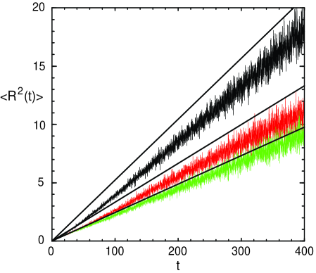
FIG. 1.: The mean-squared vortex displacement vs. time, for three different sample sizes (top to bottom): $L=6$, 12, and 24. The temperature $1/\beta=0.1$ is the same for all plots. The straight lines are the Einstein formula for pure diffusion, $\langle[{\bf R}(t)-{\bf R}(0)]^{2}\rangle=4\sigma t$, with $\sigma$ calculated from Eq. (26).

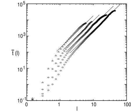
FIG. 2.: The mean first passage time vs. the box size, for four temperatures (top to bottom): $1/\beta=0.0125$, 0.025, 0.05, and 0.1. System size $L=6$ is the same for all plots. Straight lines are the theoretical predictions for pure diffusion, with $\sigma$ calculated from Eq. (26).

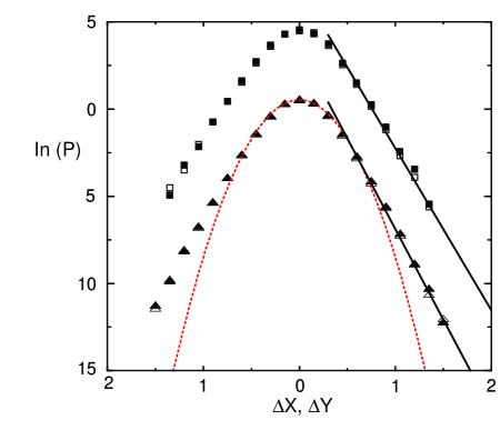
FIG. 3.: The PDF of vortex flights, for $L=6$ (triangles) and $L=12$ (squares, shifted by four orders for clarity). $1/\beta=0.1$, and time interval between measurements $\Delta t=0.1$. Full and empty symbols correspond to ${\cal P}(\Delta x)$ and ${\cal P}(\Delta y)$. The dotted line is the Gaussian distribution with the same rms deviation as the numerical data for $L=6$. The straight lines are drawn with slopes corresponding to numerical data.

REFERENCES

- [1] Present address: Institute for Pure and Applied Physical Sciences, University of California at San Diego, 9500 Gilman Dr., La Jolla, CA 92093-0360.
- [2] E.B. Sonin, Rev. Mod. Phys. 59, 87 (1987).
- [3] E.H. Brandt, Rep. Prog. Phys. 58, 1465 (1995).
- [4] D.E. Farrell, in Physical Properties of High Temperature Superconductors IV, edited by D.M. Ginsberg (World Scientific, Singapore, 1994).
- [5] N.D. Mermin, Rev. Mod. Phys. 51, 591 (1979).
- [6] M.J. Stephen and J.P. Straley, Rev. Mod. Phys. 46, 617 (1974).
- [7] F.G. Mertens, H.J. Schnitzer and A.R. Bishop, Phys. Rev. B 56, 2510 (1997).
- [8] D. Rozas, Z.S. Sacks and G.A. Swartzlander, Jr., Phys. Rev. Lett. 79, 3399 (1997).
- [9] A. Vilenkin and E.P.S. Shellard, Cosmic Strings and Other Topological Defects (Cambridge University Press, Cambridge, 1994).
- [10] See, for example, N. Grønbech-Jensen, A.R. Bishop, and D. Dominguez, Phys. Rev. Lett. 76, 2985 (1996); M.W. Coffey and J.R. Clem, ibid. 67, 386 (1991).
- [11] H.T.C. Stoof, Phys. Rev. Lett. 78, 768 (1997).
- [12] L. P. Pitaevskii, Zh. Exp. Teor. Fiz. 35, 408 (1958) [Sov. Phys. JETP 8, 282 (1959)].
- [13] E.P. Gross, Nuovo Cimento 20, 454 (1961).
- [14] A. Schmid, Phys. Kond. Mat. 5, 302 (1966).
- [15] L.P. Gor’kov and N.B. Kopnin, Usp. Fiz. Nauk 116, 413 (1975) [Sov. Phys.-Usp. 18, 496 (1976)].
- [16] L.P. Gor’kov and G.M. Eliashberg, Zh. Exp. Teor. Fiz. 54, 612 (1968) [Sov. Phys. JETP 27, 328 (1968)]; G.M. Eliashberg, ibid. 55, 2443 (1968) [ibid. 29, 1298 (1969)].
- [17] D. J. Kaup, Phys. Rev. B 27, 6787 (1983).
- [18] E. Tomboulis, Phys. Rev. D 12, 1668 (1975).
- [19] L.P. Pitaevskii, Zh. Exp. Teor. Fiz. 40, 646 (1961) [Sov. Phys. JETP 13, 451 (1961)].
- [20] C.W. Gardiner, Handbook of Stochastic Methods for Physics, Chemistry and the Natural Sciences, (Springer, New York, 1997).
- [21] E. Šimánek, Inhomogeneous Superconductors, (Oxford University Press, New York, 1994).
- [22] H. Suhl, Phys. Rev. Lett. 14, 226 (1965).
- [23] We note a conceptual similarity between our model and the random manifold problem (RMP), see M. Mézard and G. Parisi, J. Physique I 1, 809 (1991) for analysis and earlier references. The noise average in and averaging over correspond respectively to thermal and quenched disorder averaging in the RMP.
- [24] R. Bhagavatula and C. Jayaprakash, Phys. Rev. Lett. 71, 3657 (1993).
- [25] B.I. Shraiman and E.D. Siggia, Phys. Rev. E 49, 2912 (1994).
- [26] P.G. de Gennes, Superconductivity in Metals and Alloys, (Benjamin Press, New York, 1966).
- [27] We are indebted to D.P. Arovas for this observation.
- [28] P.E. Kloeden and E. Platen, Numerical solution of stochastic differential equations, (Springer-Verlag, New York, 1992).
- [29] Q. Niu, P. Ao and D.J. Thouless, Phys. Rev. Lett. 72, 1706 (1994).
- [30] J.M. Duan and A.J. Leggett, Phys. Rev. Lett. 68, 1216 (1992).
- [31] D.P. Arovas and J.A. Freire, Phys. Rev. B 55, 1068 (1997).
- [32] R.A. Siegel and R. Langer, J. Colloid Interface Sci. 109, 426 (1986).
- [33] A.M. Troyanovski, J. Aarts and P.H. Kes, Nature 399, 665 (1999).