[cond-mat/9907481] 1 Δ⁢𝐸^TBC (opne circles) and Δ⁢𝐸^PBC (closed circles) for 𝐿=18 spins as functions of anisotropy parameter Δ when 𝑡=-0.25. From the crossing point we obtain Δ

Quantum Phase Transition of $S=1/2$ Trimerized

$XXZ$ Spin Chain in Magnetic Field

^aKiyomi Okamoto and ^bAtsuhiro Kitazawa

^aDepartment of Physics, Tokyo Institute of Technology,

Oh-okayama, Meguro-ku, Tokyo 152-8551, Japan

and

^bDepartment of Physics, Kyushu University,

Hakozaki, Higashi-ku, Fukuoka 812-8581, Japan

We study the magnetization plateau at a third of the saturation magnetization of the $S=1/2$ trimerized $XXZ$ spin chain at $T=0$ . The appearance of the plateau depends on the values of the $XXZ$ anisotropy and the magnitude of the trimerization. This plateauful-plateauless transition is a quantum phase transition of the Berezinskii-Kosterlitz-Thouless type, which is difficult to precisely detect from the numerical data. To determine the phase boundary line of this transition precisely, we use the level crossing of low-lying excitations obtained from the numerical diagonalization. We also discuss the $S=1/2$ ferromagnetic-ferromagnetic-antiferromagnetic chain.

Keywords: Magnetization plateau, Quantum spin chain, Quantum phase transition

Email address: kokamoto@stat.phys.titech.ac.jp

We study the magnetization plateau at $M=M_{\rm s}/3$ ( $M_{\rm s}$ is the saturation magnetization) of the $S=1/2$ trimerized $XXZ$ spin chain described by [1]

	$\displaystyle H$	$\displaystyle=$	$\displaystyle\sum_{j=1}^{L}\left\{J^{{}^{\prime}}\left[h_{3j-2,3j-1}(\Delta)+h_{3j-1,3j}(\Delta)\right]\right.$		(1)
			$\displaystyle~{}~{}~{}~{}~{}~{}\left.+Jh_{3j,3j+1}(\Delta)\right\}$		(1)

where

h_{lm}(\Delta)=h^{\perp}_{lm}+\Delta h^{z}_{lm}

(2)

h^{\perp}_{lm}=S^{x}_{l}S^{x}_{m}+S^{y}_{l}S^{y}_{m},~{}~{}~{}h^{z}_{lm}=S^{z}_{l}S^{z}_{m}.

(3)

It is convenient to parametrize the Hamiltonian (1) as

J=J_{0}(1+2t),~{}~{}~{}~{}~{}J^{\prime}=J_{0}(1-t)

(4)

where $-1/2\leq t\leq 1$ is the trimerization parameter. The bosonized expression of the Hamiltonian (4) has the sine-Gordon form

	$\displaystyle H$	$\displaystyle=$	$\displaystyle\frac{1}{2\pi}\int dx\left[v_{\rm s}K(\pi\Pi)^{2}+\frac{v_{\rm s}}{K}\left(\frac{\partial\phi}{\partial x}\right)^{2}\right]$		(5)
			$\displaystyle~{}~{}~{}~{}~{}~{}+\frac{y_{\phi}v_{\rm s}}{2\pi}\int dx\cos\sqrt{2}\phi$		(5)

where $v_{\rm s}$ is the spin wave velocity of the system, $\Pi$ is the momentum density conjugate to $\phi$ , $[\phi(x),\Pi(x^{\prime})]=i\delta(x-x^{\prime})$ , and the coefficients $v_{\rm s}$ , $K$ , and $y_{\phi}$ are smooth functions of $J_{0}$ , $t$ and $\Delta$ The field $\phi$ is related to the fast varying (in space) part of the spin density $S^{z}(x)$ in the continuum picture as

S^{z}_{\rm fast}(x)={1\over 3}\left\{\cos\left(2k_{\rm F}x-{\pi\over 3}+\sqrt{2}\phi\right)+{1\over 2}\right\}

(6)

which makes it clear the physical meaning of $\phi$ .

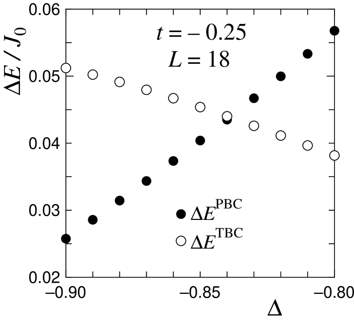
As is well known, the excitation spectrum of the sine-Gordon model is either massive (plateauful) or massless (plateauless) depending on the values of parameters. These two states are distinguished by the renormalized value of $K$ : the former is realized when $K<4$ and the latter $K\geq 4$ . The transition between these two states is of the Brerezinskii-Kosterlitz-Thouless type, which was first pointed out by one of the present authors (K.O) [2]. To determine the $K=4$ BKT transition point from the numerical diagonalization data for finite systems, we use the method developed by Nomura and Kitazawa [3]. They discussed the $K=4$ BKT transition at $M=0$ to find that the crossing between the $M=0$ excitation with the twisted boundary condition (TBC) and the $M=2$ excitation with the periodic boundary condition (PBC). Because we discuss the finite magnetization case now, it is necessary to use the Legendre transformation $E\to E-HM$ . Thus we can conclude that the crossing between

\Delta E^{\rm TBC}=E_{0}^{\rm TBC}\left(\frac{M_{\rm s}}{3}\right)-E_{0}^{\rm PBC}\left(\frac{M_{\rm s}}{3}\right)

(7)

and

\Delta E^{\rm PBC}=\tilde{E}_{0}^{\rm PBC}-E_{0}^{\rm PBC}\left({M_{\rm s}\over 3}\right)\,.

(8)

where $\tilde{E}_{0}^{\rm PBC}=(1/2)\{E_{0}^{\rm PBC}(M_{\rm s}/3+2)+E_{0}^{\rm PBC}(M_{\rm s}/3-2)\}$ . Figure 1 shows the crossing between these two excitations, from which we see $\Delta_{\rm c}(L=18)=-0.8389$ . By sweeping parameters, we obtain the phase diagram on the $\Delta-t$ plane (Fig.1).

We also investigate the ferromagnetic-ferromagnetic-antiferromagnetic model [2,4]

	$\displaystyle H_{\rm FFA}$	$\displaystyle=$	$\displaystyle\sum_{j}\left\{-J_{\rm F}\left[h_{3j-2,3j-1}(1)+h_{3j-1,3j}(1)\right]\right.$		(9)
			$\displaystyle~{}~{}~{}~{}~{}\left.+J_{\rm A}h_{3j,3j+1}(1)\right\}$		(9)

where $J_{\rm F}$ and $J_{\rm A}$ are the ferromagnetic and antiferromagnetic interaction constants, respectively. We set $\Delta=1$ so that $H_{\rm FFA}$ is reduced to the isotropic $S=3/2$ antiferromagnetic chain when $\gamma\equiv J_{\rm F}/J_{\rm A}\to\infty$ . Following Hida’s numerical calculation, the $M_{\rm s}/3$ plateau clearly exists when $\gamma\equiv J_{\rm F}/J_{\rm A}$ is small. On the other hand, it is believed that there exists no $M_{\rm s}/3$ plateau in the $S=3/2$ chain. Thus the plateauful-plateauless transition takes place at finite $\gamma$ . Since the Hamiltonian $H_{\rm FFA}$ is transformed into the generalized version of the Hamiltonian (1) by the spin rotation [2], the present method is also applicable to $H_{\rm FFA}$ , resulting in $\Delta_{\rm c}=15.4$ [5].

In conclusion, we have obtained the phase diagram for Hamiltonian (1), developing a new method to detect the plateauful-plateualess transition from the numerical diagonalization data. Our new method is applicable to various systems.

References

[1] K. Okamoto and A. Kitazawa, J. Phys. A: Math. Gen. 32 (1999) 4601.
[2] K. Okamoto, Solid State Commun. 98 (1996) 245.
[3] K. Nomura and A. Kitazawa, J. Phys. A: Math. Gen. 31 (1998) 7341.
[4] K. Hida, J. Phys. Soc. Jpn. 63 (1994) 2359.
[5] A. Kitazawa and K. Okamoto, preprint (1999).