Self-organized criticality in a model of biological evolution with long range interactions

Abstract

In this work we study the effects of introducing long range interactions in the Bak-Sneppen (BS) model of biological evolution. We analyze a recently proposed version of the BS model where the interactions decay as $r^{-\alpha}$; in this way the first nearest neighbors model is recovered in the limit $\alpha\rightarrow\infty$, and the random neighbors version for $\alpha=0$. We study the space and time correlations and analize how the critical behavior of the system changes with the parameter $\alpha$. We also study the sensibility to initial conditions of the model using the spreading of damage technique. We found that the system displays several distinct critical regimes as $\alpha$ is varied from $\alpha=0$ to $\alpha\rightarrow\infty$

In recent years an increasing numbers of systems that present Self Organized Criticality [1, 2] have been widely investigated. The general approach of statistical physics, where simple models try to catch the essencial ingredientes responsable for a given complex behavior has turned out to be very powerful for the study of this kind of problems. In particular Bak and Sneppen [3] have introduced a simple model which has shown to be able to reproduce evolutionary features such as punctuacted equilibrium [4]. Altough this model does not intend to give an accurate description of darwinian evolution, it catches into a single and very simple scheme (it is based on very simple dynamical rules) several features that are expected to be present in evolutionary processes, that is, punctuated equilibrium [3], Self Organized Criticality (SOC) [3] and weak sensitivity to initial conditions (WSIC) [5, 6] (i.e., chaotic behaviour where the trajectories depart with a power law of the time instead of exponentially). In this sense, one important question arises about the robustness of such properties against modifications (i.e., complexifying) of the simple dynamical rules on which the model is based. The original model, hereafter referred as the first nearest neighbors (FNN) version [3], includes only nearest neighbors interactions in a one dimensional chain. This model presents SOC [3] and weak sensitivity to initial conditions [5, 6]. On the other hand, another version of the model with interactions between sites randomly chosen in the lattice (and therefore it can be regarded as a mean field version of the FNN), hereafter referred as the random negihbors (RN) version [7], does not present SOC [8]. Moreover, it is not expected (and we shall show in this work that it is indeed the case) to present WSIC.

Systems of coevolutionary species are expected to have some distance decaying interactions, thus lying somehow between the two previous schemes. Although not well defined, the concept of “distance” between species in these scenarios may be regarded as associated to some complex network of relationships including competition for resources and predator-prey ones, among many others[9]. In this sense, the environmental modifications produced by the extinction of one species may be expected to affect many others not directly related to it, where the intensity of such influence depends on the above mentioned distance.

Along this line, in this letter we will focuse on the robustness of the SOC and sensitivity to initial conditions properties of the Bak and Sneppen model against the introduction of long-range distance dependent interactions. To this end, we consider a generalization of the model, recently proposed by Cafiero et al [10] that takes into account long-range interactions between species that decay as $r^{-\alpha}$, where $r$ represent the distance between species (mesured in lattice units, i.e., $r=1,2,\ldots$ in a chain) and $\alpha>0$ is a parameter that control s the effective range of the interactions. The major value of this generalization, unlike others introduced in the literature [11, 12], resides in the fact that it allows simply to retrieve the two above mentioned models by varying continuously the parameter $\alpha$: when $\alpha\rightarrow 0$ we recover the RN version while for $\alpha\rightarrow\infty$ we recover the FNN one.

The model consist of an $N$-site linear lattice with periodic boundary conditions (i.e., a ring of $N$ sites), where each site represents a species. Each species has associated a real variable $b_{j}$, $0\leq b_{j}\leq 1,$ that measures the relative fitness barrier. Starting from a random barrier distribution, at each successive time step we identify the smallest barrier $b_{j}$, and modify it by choosing a new random value from a uniform distribution. This change represents a jump of a species across its fitness barrier to a mutated species. This mutation must also affect other species in the chain, and to take into account this phenomena one defines a neighborhood which will also be modified in the same way. In Ref. [3] ($\alpha\to\infty$) the authors considered the case in which this neighborhood consists of the two nearest species of the mutating one while in Ref. [7] ($\alpha=0$) the neighborhood consist of $K-1$ species chosen at random among all the species of the chain.

In order to generalize these models, we choose the neighborhood (of $K-1$ species) at random with a probability that decays as $r_{ij}^{-\alpha}$, where $r_{ij}$ is the distance of a given species $j$ to the species with the smallest barrier $i$, and giving them new random values chosen from a uniform distribution. In this way,for $K=3$ and $\alpha\to\infty$ we recover the two nearest neighbors model, while for $\alpha=0$ we reproduce the random neighbors mean field version.

To determine whether the system attains a self-organized critical state, we analyze the following quantities: the barrier distribution $P(b)$ in the final steady state, the spatial correlation $C(r)$ and the first return time distribution $C(t)$. In order to study the sensitivity to initial conditions, we calculate the time evolution of the Hamming distance $D(t)$ between two different replicas submitted to the same noise (damage spreading method).

Since our main interest is to analyze the crossover between the limits $\alpha=0$ and $\alpha\rightarrow\infty$, we will restrict ourselves to consider the $K=3$ case. Latter on we will discuss briefly the effect of increasing $K$. Figure 1 presents the distribution $P(b)$ of barrier values, for three different $\alpha$ values. Note that, independently of $\alpha$ the curves are qualitatively similar. The typical behavior of these curves can be characterized by the value of $P(b(1))$ (i.e, the saturation value of the distribution), which is displayed in Fig.2 as a function of $\alpha$ for three different system sizes. We can clearly distinguish three different regimes. For $\alpha<1$ the value of $P(b(1))$ is independent of $N$ and the behavior observed for $P(b)$ colapses to the one observed in the RN Bak-Sneppen model. There exists some value $\alpha=\alpha_{c}$ such that for intermediate values $1<\alpha<\alpha_{c}$ the value of $P(b(1))$ is very sensitive to changes in $\alpha$, increasing its value as $\alpha$ grows, and finally, for $\alpha>\alpha_{c}$, $P(b(1))$ reaches a saturation value, and we recover the behavior of $P(b)$ for the FNN model when $N\rightarrow\infty$. The value of $\alpha_{c}$ can be roughly estimated from numerical extrapolations of the curves to $1/N\rightarrow 0$. We obtained that $\alpha_{c}\approx 4$ for $K=3$ (further analysis of the critical exponents will confirm this estimation).

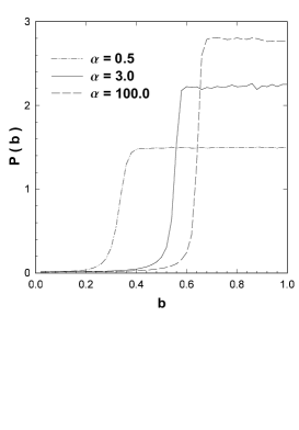
FIG. 1.: Distribution of barrier values for three different values of $\alpha:0.5,3.0$, and $100.0$. All cases have $N=250$.

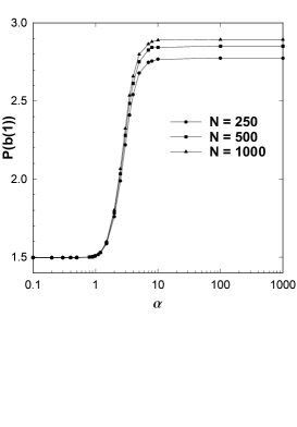
FIG. 2.: $P(b(1))$ vs $\alpha$ for three different system sizes $N=250,500$, and $1000$.

We consider now the spatial and temporal correlations between the minimum barriers in order to determine the presence of SOC. Figure 3 presents in a log-log plot the probability $C(r)$ that the minimum barriers at two succesive updates will be separated by $r$ sites. We observed a power law behavior $C(r)\sim r^{-\pi}$ for all $\alpha\neq 0$. In Fig. 4 we present how $\pi$ changes with $\alpha$. When $\alpha=0$ the spatial correlation is constant ($\pi=0$) as in the RN model. As $\alpha$ grows $\pi$ increases until it reaches a saturation value $\pi=3.2\pm 0.2$ for $\alpha>\alpha_{c}$, in agreement with the results observed in the FNN model.

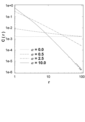
FIG. 3.: Log-log plot of the space correlation $C(r)$, for four different values of $\alpha:0.0,0.5,2,5$, and $10.0$. The system size is $N=1000$

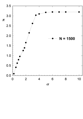
FIG. 4.: Space correlation exponent $\pi$ vs $\alpha$.

Next we calculate the first return time distribution $C(t)$, defined as the probability that, if a given site is the minimum at time $t_{0}$, it will again be the minimum for the first time at time $t_{0}+t$. In Fig. 5 we present our results for four different values of $\alpha$ (0.5, 1.5, 2.0 and 3.0). For $\alpha\geq 2$ the first return time clearly presents a power law behavior $C(t)\sim t^{-\tau}$, even for finite system sizes.

For $\alpha<2$ the system displays finite size effects, as can be seen in Fig. 6 where we present $C(t)$ when $\alpha=0.5$ for different system sizes; it is clear that a power law decay emerges as $N$ grows.

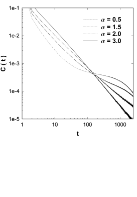
FIG. 5.: Log-log plot of the first return probability $C(t)$, for four different values of $\alpha:0.5,1.5,2.0$, and $3.0$. System size is $N=1000$

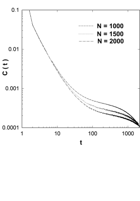
FIG. 6.: Log-log plot of the first return probability $C(t)$, for $\alpha=0.5$, for three different sizes, $N=1000,1500$, and $2000$.

In Fig. 7 we show how the first return time exponent $\tau$ depends on $\alpha$. Here again we find three different regimes: For $\alpha<1$ (unlike the spatial correlation exponent) all the curves $C_{\alpha}(t)$ colapse and $\tau=1.5$, displaying the same behavior found in the RN Bak-Sneppen model with $K=3$, where $\tau=3/2$ exactly [8]. For $1<\alpha<\alpha_{c}$, the value of $\tau$ strongly depends on the value of $\alpha$, with a minimum for $\alpha\approx 1.6$, in agreement with the results of Cafiero et al [10]. For $\alpha>\alpha_{c}$ the value of $\tau$ attains a saturation value $\tau=1.56\pm 0.05$ in agreement with the value observed in the FNN Bak-Sneppen model where $\tau=1.6$.

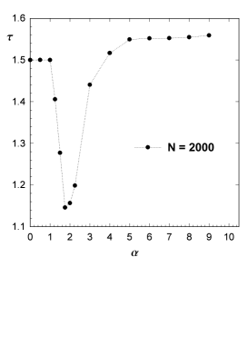
FIG. 7.: First return probability exponent, $\tau$, as a function of $\alpha$.

Summarizing the results displayed in these figures, for $0<\alpha<1$, since $\tau$ presents the same trivial value observed in the RN Bak-Sneppen model, we cannot regard the system as critical [8]. For $1<\alpha<\alpha_{c}$ the exponents depend strongly on $\alpha$, and since the exponents are non trivial, we regard this as a strong indicator of criticality in the system. Finally for $\alpha>\alpha_{c}$ the exponents becomes independent of $\alpha$, taking the short range values observed in the FNN Bak-Sneppen model. We have observed that as we increase the number of interacting sites $K$, the value of $\alpha_{c}$ decreases, slowly converging to $\alpha_{c}=2$. This behavior reminds that of the one dimensional ferromagnetic Ising model with the same type of interactions presented here, where the borderline between short and long range critical regimes is $\alpha=2$ [13].

Next, we study the sensibility to initial conditions of this model and its dependence on $\alpha$. To do that, we use the spreading of damage technique, which had previouly been applied to the FNN model [5, 6]. In this particular limit it was shown that the system presents a weak sensivity to initial conditions, characterized by a power law increment, as times goes on, of the Hamming distance between replicas of the system. This behavior is reminiscent of those observed at the edge of chaos in dynamical systems with few degrees of freedom. The procedure is as follows: given a configuration of $N$ barrier values $(\{b_{j}^{(1)}\})$ in the self-organized critical state, we create a replica of the system $(\{b_{j}^{(2)}\})$ by choosing a site randomly and interchanging the value of this site with the value of the site with the smallest barrier. From then on we use the same random numbers for updating the barrier values in both replicas.

We define the Hamming distance between the two replicas as:

$$D(t)\equiv\frac{1}{N}\sum_{j=1}^{N}|\;b_{j}^{(1)}(t)-b_{j}^{(2)}(t)\;|$$ (1)

If the Hamming distance goes to zero we say that the system is in a frozen phase. On the other hand if the Hamming distance remains non zero we say that the system is chaotic in analogy with dynamical systems.

Regarding the behavior of the average normalized Hamming distance $D(N,t)\equiv\left<D(t)\right>/\left<D(1)\right>$, we observed two different regimes as $\alpha$ is varied. For $\alpha<2$, $D(N,t)$ reaches a saturation value $D(N,\infty)$ in just one step. The quotient $D(N,\infty)/N\rightarrow 0$ when $N\rightarrow\infty$, and therefore the system does not present sensibility to the initial conditions.

The typical temporal behaviour of $D(N,t)$ for $\alpha\geq 2$ is displayed in Fig.8 for $\alpha=2.5$ and three different system sizes (the results presented correspond to averages over $500*N$ realizations). We see that $D(N,t)\sim t^{\delta}$ when $t\ll N$ and it saturates into a system size dependent value for large times, clearly showing WSIC [5, 6]. Moreover, we verified for $\forall\alpha\geq 2$ the finite size scaling behavior [5]:

$$D(N,t)\sim N^{z\delta}\;F\left(\frac{t}{N^{z}}\right)$$ (2)

where $\delta=0.40$ [14], and $z=1.7\pm 0.2$ is the dynamical exponent defined by $t_{s}\sim N^{z}$, $t_{s}$ being the value of $t$ at which the increasing regime crosses over onto the saturation regime [15] (given by the intersection of the linearly increasing branch of the curve and the horizontal branch). Both exponents are independent of $\alpha$.

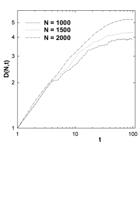
FIG. 8.: Normalized Hamming distance $D(N,t)$ for $\alpha=2.5$ and three system sizes, $N=1000,1500$, and $2000$.

Concluding, we have studied how long range interactions affects the criticality of the stationary state of our model and its sensibility to the initial conditions. Concerning the SOC, we observed three different regimes depending on $\alpha$. For $\alpha>\alpha_{c}$ we can speak about a short-range critical regime, where the system presents SOC. Moreover, we observe that this property displays universality, in the sense that most of the associated critical exponents are independent of $\alpha$. For $0\leq\alpha\leq 1$ the system does not present SOC, although $C(r)$ displays a non-trivial power law decay with $r$, unlike the RN model for wich $C(r)$ is constant. Moreover, all the relevant state functions or distributions become independent of $\alpha$. This behavior has already been observed in a variety of systems with long-range interactions, both related to equilibrium [16, 17] and non-equilibrium properties [18, 19]. In all these systems it has been observed that the mean field behavior becomes dominant when $0\leq\alpha\leq d$, $d$ being the dimensionality of the underlying lattice. Hence, in our case we can speak about a “mean-field” (non-critical) regime, i.e., that of the RN model. Finally, for $1\leq\alpha\leq\alpha_{c}$ we have a long-range critical regime, where the system presents non-universal SOC, i.e., the associated critical exponents depend strongly on $\alpha$.

Concerning the sensibility to the initial conditions we observed two regimes: one for $0\leq\alpha<2$ where the system does not present sensibility to the initial conditions of any type, while for $\alpha>2$ it displays universal WSIC, in the sense that the exponents of the scaling law (2) are independent of $\alpha$.

We see that, at least one of the borderline values (and probably all of them) that separate the different regimes seems to be directly related to the dimensionality of the system. Hence, such dimensionality appears as a fundamental parameter to determine the robustness of the model against variations in the range of the interactions.

Fruitful discussions and suggestions from S. Boettcher are acknowledged. This work was partially supported by the following agencies: CONICOR (Córdoba, Argentina), Secretaria de Ciencia y Tecnología de la Universidad Nacional de Córdoba and CONICET (Argentina).

REFERENCES

- [1] P. Bak, C. Tang, and K. Wiesenfeld. Phys. Rev. Lett. 59, 381 (1987).
- [2] P. Bak, C. Tang, and K. Wiesenfeld. Phys. Rev. A 38, 364 (1988).
- [3] Per Bak and Kim Sneppen Phys. Rev. Lett. 71, 4083 (1993).
- [4] S. J. Gould, Paleobiology 3, 135 (1977).
- [5] F. A. Tamarit, S. A. Cannas and C. Tsallis Eur. Phys. J. B. (1998).
- [6] A. Valleriani and José Luis Vega, J. Phys. A 32, 105 (1999).
- [7] H. Flyvbjerg, P. Bak and K. Sneppen Phys. Rev. Lett. 71, 4087 (1993).
- [8] Jan de Boer, A. D. Jackson, and Tilo Wettig Phys. Rev. E 51, 1059 (1995).
- [9] K. Havens, Science 257, 1107 (1992).
- [10] R. Cafiero, P. De Los Rios, A. Valleriani and J. L. Vega. cond-mat/9906337
- [11] N. Vandewalle and M. Ausloos. Phys. Rev. E 57, 1167 (1998).
- [12] R. Cafiero, P. De Los Rios, F-M Dittes, A. Valleriani, J. L. Vega. Phys. Rev. E 58, 3993 (1998).
- [13] F. J. Dyson, Commun. Math. Phys. 12, 91 (1969); F. J. Dyson, Commun. Math. Phys. 12, 212 (1969).
- [14] R. Cafiero, A. Valleriani and José Luis Vega, cond-mat/9906427.
- [15] F. Wang, N. Hatano and M. Suzuki, J. Phys. A 28, 45443 (1995).
- [16] S. A. Cannas and F. A. Tamarit, Phys. Rev. B 54, R12661, (1996).
- [17] S. A. Cannas, A. C. N. de Magalhaẽs and F. A. Tamarit, submitted;cond-mat/9906340.
- [18] S. A. Cannas, Physica A 358, 32 (1998).
- [19] C. B. Anteneodo and C. Tsallis, Phys. Rev. Lett. 80, 5313 (1998); C. B. Anteneodo and F. A. Tamarit, submitted.