Umklapp scattering in transport through a 1D wire of finite length.

Abstract

Suppression of electron current $\Delta I$ through a 1D channel of length $L$ connecting two Fermi liquid reservoirs is studied taking into account the Umklapp interaction induced by a periodic potential. This interaction opens band gaps at the integer fillings and Hubbard gaps $2m$ at some rational fillings in the infinite wire: $L\to\infty$. In the perturbative regime where $m\ll v_{c}/L$ ($v_{c}:$ charge velocity), and for small deviations $\delta n$ of the electron density from its commensurate values $-\Delta I/V$ can diverge with some exponent as voltage or temperature $V,T$ decreases above $E_{c}=max(v_{c}/L,v_{c}\delta n)$, while it goes to zero below $E_{c}$. This results in a non-monotonous behavior of the conductance. In the case when the Umklapp interaction creates a large Mott-Hubbard gap $2m\gg T_{L}$ inside the wire, the transport is suppressed near half-filling everywhere inside the gap except for an exponentially small region of $V,T<T_{L}exp(-2m/T_{L})$.

I Introduction

Recent developements in the nano-fabrication technique have made the 1D interacting electron systems an experimental reality, and its quantum transport properties have been the subject of extensive studies both experimentally [1-3] and theoretically [4-16]. In realistic experimental set-ups, the quantum wire is attached to two-dimensional regions called reservoirs or leads. A metallic phase of the infinite wire is known as a Tomonaga-Luttinger liquid [14]. To describe 1D transport phenomena in the realistic configuration a model was recently formulated of the inhomogeneous Tomonaga-Luttinger liquid (ITTL) [4, 5, 6]. It recovers the conductance $G=2e^{2}/h$ observed experimentally even in the presence of the electron-electron interaction in the wire [1] (below we use the units, where $e=\hbar=1$), although the previous calculations on an infinitely long wire [7, 8] predicted the renormalized conductance ( see [9] for the further development). Calculation of the conductance suppressed by a weak random impurity potential in this model [10] had agreed with both the previous theoretical prediction [8] and an experiment [1].

In this paper we consider effect of opening a spectral gap in the wire on the 1D transport. Theory [11] predicts that in 1D besides band gaps produced by a periodical potential in the wire at the integer fillings, a repulsive interaction between electrons opens Mott-Hubbard gaps at some rational fillings. Furthermore recently Tarucha et al. [17] succeeded in introducing the 1D periodic potential with a periodicity of order 40nm into the wire 2$\mu$m in length and 50nm wide. This induces Umklapp scattering. The electron density $n$ can be continuously controlled by the gate voltage, and one can satisfy the half-filling condition within an accessible value of $n$. If this condition is satisfied the system will becomes a 1D (doped) Mott insulator with the Mott-Hubbard gap $m$ for the infinite length wire. Then it will offer an idealistic system to study the quantum transport in Mott and doped Mott insulators in 1D. Earlier a similar experiment had been carried out by Kouwenhoven at al [3]. Their wire was 3$\mu$m in length, 250-400nm wide and the period of the structure 200nm. To reduce the impurity backscattering they put the set-up in a strong magnetic field and observed an interference structure at the integer edge-state plateaus in conductance vs. gate voltage. This structure partly had been explained as a band gap appearance.

Inspired by these works, we study theoretically the $I-V$ characteristic of the wire of length $L$ connected to leads at different temperatures $T$ taking into account the Umklapp electron-electron interactions, which can be directly compared with the experiments. We formulate our model in the section II and check it on the description of the band gap effect at different temperatures. We calculate [18] the suppression of the current $\Delta I$ perturbatively in the Umklapp scatterings in the section III. The results are summarized in Figs. 1 and 2 for a threshold structure near half filling. There are two energy scales, i.e., the finite size energy $T_{L}=v_{c}/L$ ($v_{c}:$ charge velocity) and $E_{thr}\sim v_{c}\delta n$ ($\delta n:$ the deviation of the electron density from its value at the filling $\nu$ equal to $1/2$) measuring the incommensurability. For $T,V>E_{c}=max(v_{c}/L,E_{thr})$, the suppression of the current $-\Delta I/V$ diverges as $max(T,V)^{4g-3}$ if the short range interaction constant $g$ for the forward scattering is less than $3/4$. For $T,V<E_{c}$, on the other hand, the suppression $-\Delta I/V$ goes to zero as $T,V\rightarrow 0$. Then we predict the non-monotonous temperature and/or voltage dependence of $I$, which is the clear signature of the Umklapp scattering effect. For small values of $g$, expected when the screening length $\xi_{c}$ of the interaction determined by the close metallic gates is much larger than the width of the channel $d$ and $g\propto 1/\sqrt{\ln\xi_{c}/d}$ [12], we predict a few more threshold singularities. These features could be observed experimentally by changing the gate voltage, bias voltage, and temperature.

In the next section IV, motivated by a recent discussion [19, 20] that in a non-perturbative case of the large Mott-Hubbard gap $2m\gg v_{c}/L\equiv T_{L}$ the conductance is strongly suppressed at any low energy (¡$m$) inside the gap similar to the band gap case, we consider transport through a 1D Mott-Hubbard insulator of a finite length $L$ beyond perturbative approach. Our presentation follows [22] where we used a special value of the low energy constant of the interaction to map the problem onto the exactly solvable models. We find current vs. voltage $V$ at high temperature $T>max(m,T_{L})$ and at low energy $T,V<T_{L}$. The result shows that for the strong interaction creating a large Mott-Hubbard gap $2m\gg T_{L}$ inside the wire, the transport is suppressed near half-filling everywhere inside the gap except for an exponentially small region of $V,T<T_{L}exp(-2m/T_{L})$

II Model

Our model can be derived following [5] from a 1 channel electron Hamiltonian

$${\cal H}=\int d\!x\{\sum_{\sigma}\psi_{\sigma}^{+}(x)(-\frac{\partial^{2}_{x}}{2m^{*}}-E_{F})\psi_{\sigma}(x)$$ (2)

$$\hskip 28.45274pt+\varphi(x)\rho^{2}(x)+[V_{imp}(x)+V_{period}(x)]\rho(x)\}$$

with the periodic potential $V_{period}(x)$ ( period $a$) assumed to be weak enough to justify the perturbative consideration of the Umklapp backscatterings. The Fermi momentum $k_{F}$ and the Fermi energy $E_{F}$ is determined by the filling factor $\nu$ as $\nu=k_{F}a/\pi$ and $E_{F}\approx v_{F}k_{F}$. In Eq. (2) the function $\varphi(x)=const\times\theta(x)\theta(L-x)$ switches on the electron-electron interaction inside the wire confined in $0<x<L$. This interaction is assumed to be local, as the close metallic gate used in experiments to form the wire inevitably screens the long range Coulomb. Contribution of the random impurity potential $V_{imp}(x)\rho(x)$ to the conductance has been considered in [8, 10], some results of which we will use below. Following Haldane’s generalized bosonization procedure [14] to account for the nonlinear dispersion one has to write the fermionic fields as $\psi_{\sigma}(x)=\sqrt{k_{F}/(2\pi)}\sum exp\{i(n+1)(k_{F}x+\phi_{\sigma}(x)/2)+i\theta_{\sigma}(x)/2\}$ and the electron density fluctuations as $\rho(x)=\sum\rho_{\sigma}(x),\ \rho_{\sigma}(x)=[\partial_{x}\phi_{\sigma}(x)+2k_{F}]/(2\pi)\sum exp\{in(k_{F}x+\phi_{\sigma}(x)/2)\}$ where summation runs over even $n$ and $\phi_{\sigma},\theta_{\sigma}$ are mutually conjugated bosonic fields $[\phi_{\sigma}(x),\theta_{\sigma}(y)]=i2\pi sgn(x-y)$.

After substitution of these expressions into (2) and introduction of the charge and spin bosonic fields as $\phi_{c,s}=(\phi_{\uparrow}\pm\phi_{\downarrow})/\sqrt{2}$ the Hamiltonian takes its bose-form ${\cal H}={\cal H}_{O}+{\cal H}_{bs}$. Here the free electron movement modified by the forward scattering interaction is described by [4, 5, 6]

$${\cal H}_{O}=\int dx\sum_{b=c,s}\frac{v_{b}}{2}\{{1\over{g_{b}(x)}}\left({{\partial_{x}\phi_{b}(x)}\over{\sqrt{4\pi}}}\right)^{2}$$ (4)

$$\hskip 113.81102pt+g_{b}(x)\left({{\partial_{x}\theta_{b}(x)}\over{\sqrt{4\pi}}}\right)^{2}\}$$

with $g_{c}(x)=g$ for $x\in[0,L]$ ( $g$ is less than 1 for the repulsive interaction and it will be assumed below ), $g_{c}(x)=1$, otherwise and $v_{c}(x)=v_{F}/g_{c}(x)$. The constants in the spin channel $g_{s}=1,v_{s}=v_{F}$ are fixed by $SU(2)$ symmetry. Keeping only the most slowly decaying terms among others with the same transferred momentum one could write the backscattering interaction as

                                                                           

$${\cal H}_{bs}={E_{F}^{2}\over v_{F}}\int_{0}^{L}dx\bigl{[}\sum_{even\ m>0}U_{m}\cos(2k_{mF}mx+{{m\phi_{c}(x)}\over\sqrt{2}})+\sum_{odd\ m>0}U_{m}\cos({\phi_{s}(x)\over\sqrt{2}})cos(2k_{mF}mx+{{m\phi_{c}(x)}\over\sqrt{2}})\bigr{]}$$ (5)

                                                                           

A difference in the transferred momentums $2k_{mF}$ is brought by the periodical potential with the period $a$: $k_{mF}=k_{F}-\pi l/(ma))$, where $l$ is an integer chosen to minimize $|k_{mF}|$. We have omitted the $m=0$ term of the first sum: It can contain only the spin field and cannot affect the current in the lowest perturbative order. The most singular is the $m=1$ term of the second sum responsible for opening the band gap in the infinite wire at $\nu=integer$. The dimensionless coefficients $U_{m}$ originate from $\varphi(x)$.

In the spinless case we should put $\phi_{c}=\phi_{\sigma}$ in (4) and change the backscattering interaction to

                                                                           

$${\cal H}_{bs}={E_{F}^{2}\over v_{F}}\int_{0}^{L}dx\sum_{m>0}U_{m}\cos(2k_{mF}mx+m\phi_{\sigma}(x))$$ (6)

                                                                           

To generalize our perturbative results of the part III to the spinless case one just needs to transform $m,k_{mF}$ to $\sqrt{2}m,k_{mF}/\sqrt{2}$ in the expressions written in the spin case for even $m$ and take $m$ arbitrary integer.

It is instructive first to examine how the band gap shows out in transport properties of the wire filled with the non-interacting electrons. The model is equivalent to a Dirac equation with the mass switched on inside the wire:

                                                                           

$${\cal H}_{D}=i\sum_{a=R,L=\pm}\psi^{+}_{a}(\mp v_{c}\partial_{x})\psi_{a}-m\varphi(x)[e^{i2k_{F}x}\psi^{+}_{L}(x)\psi_{R}(x)+h.c.]$$ (7)

                                                                           

with $m=\pi E_{F}U_{1}/2$ in the spin case of Eq. (5) and $m=\pi E_{F}U_{1}$ in the spinless case of Eq. (6). Here $\psi_{R(L)}$ describes the right (left) chiral electron and $k_{F}$ is counted from $\pi l/a$ at $\nu\simeq l$. The transport is determined by the transmittance $D$ which is a function of the electron energy $\varepsilon$ counted from the one of the middle of the gap $v_{F}\pi l/a$ :

$$D(\varepsilon)=\left[1+m^{2}{\sin^{2}(\sqrt{\varepsilon^{2}-m^{2}}t_{L})\over\varepsilon^{2}-m^{2}}\right]^{-1}$$ (8)

where the analytical extension is assumed at $\varepsilon<m$ and $t_{L}=L/v_{F}$. In particular, the linear bias conductance $G$ is equal to

$$G(T,\mu_{0})={1\over 2\pi T}\int d\varepsilon\frac{D(\varepsilon)}{1+\cosh((\varepsilon-\mu_{0})/T)}$$ (9)

for spin electrons where $\mu_{0}=k_{F}v_{F}$ gives a deviation of the chemical potential of the wire from that of the $\nu=l$ filling. The conductance has two regimes of behavior.

1. High temperatures $T>T_{L},m$ - The asymptotics to (9) can be written as

$$G={1\over\pi}\left(1-{m\over 2T}\frac{B(m/T_{L})}{1+\cosh(\mu_{0}/T)}\right)$$ (10)

after noticing that $D$ is a quickly oscillating function against the slowly varying temperature factor. The coefficient $B$ changes slowly from 0 to $\simeq\pi$ and is defined below in Eq. (28). The expression (10) shows that at the high temperature the band gap produces a smooth well in the conductance vs. chemical potential which becomes more narrow and deeper as $T$ decreases.

2. Low temperatures $T<T_{L}$- The conductance is about $D(\mu_{0})/\pi$. It is suppressed in the middle of the gap $G(0)=\left[\pi(1+(mt_{L})^{2})\right]^{-1}$ and approach its maximum $1/\pi$ away from the gap oscillating with period $\pi/t_{L}$. In the limit $mt_{L}\ll 1$ this interference structure is perfectly periodical, as

$$\Delta G_{1}=-(mt_{L})^{2}\frac{\sin^{2}((k_{F}-\pi l/a)L)}{((k_{F}-\pi l/a)L)^{2}}$$ (11)

Therefore the conductance has $L/a$ humps in between two neighbor band gaps. We expect this being correct at any finite $m$ from comparison with a tight binding model. In our model it holds on asymptotically if $\pi v_{c}/(am)\gg 1$. Then the model works well.

III Narrow gap: perturbative approach

In this section we assume that the dimensionless coefficients $U_{m}$ in Eq.(5) are small enough to justify perturbative calculation of the current. The variation of the current due to the backscattering is given by : $\Delta\!I=-i/(2\sqrt{2}\pi)\int d\!x\,[\partial_{x}\theta_{c}(x),{\cal H}]=\sqrt{2}\int d\!x(\delta/\delta\!\phi_{c}(x)){\cal H}_{bs}$. At finite voltage $V$ applied symmetrically to neglect the momentum transfer variation, the average of $\Delta\!I$ decomposes into sum of the different backscattering mechanism contributions $<\Delta\!I_{m}>$ in the lowest order. The even $m$ terms involving only $\phi_{c}$ field are equal to

                                                                           

$$<\Delta\!I_{m}>=-{m\over 4}\bigl{(}{{U_{m}E_{F}^{2}}\over v_{F}}\bigr{)}^{2}\int_{-\infty}^{\infty}dt\int\!\int_{0}^{L}d\!x_{1}d\!x_{2}<e^{im\phi_{c}(x_{1},t)/\sqrt{2}}e^{-im\phi_{c}(x_{2},0)/\sqrt{2}}>\bigl{[}e^{im(2k_{mF}(x_{1}-x_{2})+Vt)}-h.c.\bigr{]}.$$ (12)

                                                                           

The current operator $\Delta\!I_{m}$ has a high energy scaling dimension $m^{2}g/2$ and a free electron ($g=1$) behavior at low energy. We will see below that the integral (12) scales at low energy with $(m^{2}-1)$ exponent and with $(m^{2}g-2)$ exponent at high energy. The most singular behavior is due to Umklapp backscattering at $m=2$ with the threshold voltage $V=E_{thr}=2k_{2F}v_{c}$ going to zero at the half filling. We assume $V,E_{thr}\geq 0$ below. Less singular correction with $m=4$ could become relevant at the one and three quarters fillings and so on. Expressions for the odd $m$ terms include additionally a spin field correlator $<e^{i\phi_{s}(x_{1},t)/\sqrt{2}}e^{-i\phi_{s}(x_{2},0)/\sqrt{2}}>$ under the integrals in (12). The high energy dimension of $\Delta\!I_{m}$ in this case is $m^{2}g/2+1/2$. The most singular behavior occurs to the $m=3$ term at the one and two thirds fillings. It has two threshold energies $E_{thr\,c,s}=2k_{3F}v_{c,s}$ for $v_{c}\neq v_{s}$. Neglecting a change of the TLL compressibility produced by the Umklapp scattering we can relate [23] the threshold energy to a deviation of the chemical potential of the wire $\mu$ at $V=0$ from that of the rational filling. Since $\Delta\rho_{c}=2k_{F}/\pi$ and $\partial\mu/\partial\rho_{c}=\pi v_{c}/(2g)$ we gather $E_{thr,c}=2g\mu$. However, in an experiment it is the average of the electrochemical potentials of the leads but not $\mu$ that is known. The latter is proportional to $\mu$ with the coefficient $[1+2ge^{2}/(\pi v_{c}\hbar c_{g})]$ if the gate voltage is fixed [23]. This coefficient is about $1$ if the density $c_{g}$ of the capacitance between the wire and the screening gate is large.

Correlator of the charge field exponents $e^{i\phi_{c}(x,t)}$, evolution of which is specified by ${\cal H}_{O}$, could be compiled from the correlators of the uniform TL liquid $K(x,t)=K(x,t,g,v_{c})$ ($K(x,t,g,v)\equiv(\alpha\pi/\beta)^{2g}/(\prod_{\pm}\sinh^{g}(\pi(x/v\pm(t-i\alpha))/\beta)))$ in the following way [4, 10]

                                                                           

$$<e^{i\phi_{c}(x,t)}e^{-i\phi_{c}(y,0)}>=K(x-y,t)\prod_{\pm,n=1}^{\infty}\bigl{(}{{K(2nL,0)}\over{K(2nL\pm\mid x-y\mid,t)}}\bigr{)}^{-r^{2n}}$$ (14)

$$\hskip 42.67912pt\times\prod_{n=0}^{\infty}\bigl{(}{{K(2(nL+x),0)K(2(nL+y),0)}\over{K^{2}(2nL+x+y,t)}}\bigr{)}^{-r^{2n+1}/2}\prod_{n=1}^{\infty}\bigl{(}{{K(2(nL-x),0)K(2(nL-y),0)}\over{K^{2}(2nL-x-y,t)}}\bigr{)}^{-r^{2n-1}/2},$$

                                                                           

Here $\beta$ is inverse temperature $1/T$ and $\alpha=1/E_{F}$ is the ultraviolet cut-off. This complicated form comes about through a multiple scattering at the points of joint $x=0,L$. As a result of the scattering the correlator $<\phi_{c}(x,t)\phi_{c}(y,0)>$ becomes an infinite sum of the uniform correlators taken along the different paths connecting points x and y and undergoing reflections from the boundaries at $x=0,L$. Each reflection brings additional factor $r=(1-g)/(1+g)$. The similar correlator $<e^{i\phi_{s}(x,t)}e^{-i\phi_{s}(y,0)}>$ for spin field is $K(x-y,t,1,v_{s})$. Below we analyze the current corrections (12) for high ($T>1/t_{L}=T_{L}$) and low ($T\ll T_{L}$) temperatures, respectively.

1.High temperatures $T>T_{L}$ - The uniform correlator $K(x,t)$ goes down exponentially if distance between the points $\mid x\mid$ exceeds the inverse temperature. Therefore only paths with length less than $\beta$ contribute to the correlator (14). This means that the high temperature form of the correlator (14) reduces to the first multiplier $K(x-y,t)$ up to a factor $(1+O(exp(-t_{L}/\beta))$. Neglecting $O(T_{L}/T)$ quantity we can extend integration over $x_{1}-x_{2}$ in (12) from $-\infty$ to $+\infty$. Then calculation of the $m=2$ contribution reduces to finding Fourier transformation $F_{2g}(q,\varepsilon)$ of the correlator $K^{2}(x,t,g,v_{c})$:

                                                                           

$$<\Delta\!I_{2}>={1\over 4}\left({{U_{2}E_{F}^{2}}\over g}\right)^{2}t_{L}\sum_{\pm}\mp F_{2g}(2E_{thr},\pm 2V)=-2\bigl{(}{{2^{2(g-1)}U_{2}}\over{\Gamma(2g)g}}\bigr{)}^{2}{E_{F}^{2}\over T_{L}}\bigl{(}{{\pi T}\over E_{F}}\bigr{)}^{4g-2}\sinh({V\over T})\prod_{\pm,\pm}\Gamma(g\pm i{{V\pm E_{thr}}\over{2\pi T}})$$ (15)

One can easily see its behavior making use of the following asymtpotics:

$$<\Delta\!I_{2}>\propto-\left({U_{2}\over g}\right)^{2}{E_{F}^{2}\over T_{L}}\left\{\matrix{((V^{2}-E_{thr}^{2})/E^{2}_{F})^{2g-1},&V\gg E_{thr},\ T\cr((V+E_{thr})T/E^{2}_{F})^{2g-1},\ \ &V\approx E_{thr}\gg T\cr}\right.$$ (16)

$$<\Delta\!I_{2}>\propto-\left({U_{2}\over g}\right)^{2}{E_{F}^{2}\over T_{L}}\sinh{V\over T}\left\{\matrix{e^{-E_{thr}/T}((E_{thr}^{2}-V^{2})/E^{2}_{F})^{2g-1},\ \ &E_{thr}\gg V,\ T\cr(T/E_{F})^{4g-2},&V\ ,E_{thr}\ll T\cr}\right.$$ (17)

                                                                           

FIG. 1.: Schematic voltage dependence of the high temperature current corrections produced by the $m=2$ Umklapp interaction $\Delta I_{2}$. Solid lines, $E_{thr}=0$; dashed lines, $E_{thr}\gg T$.

These asymptotics show that the threshold singularity in the current voltage dependence diverges as $((V-E_{thr})/T)^{2g-1}$ if $g<1/2$ (Fig.3). It becomes stronger in the differential conductance dependence. At $g>1/2$ the differential conductance correction $d\!G_{2}$ behaves as $-(V/E_{F})^{4g-3}$, and saturates at $-(T/E_{F})^{4g-3}$ below $T$, if $E_{thr}<T$; otherwise, the correction shows divergence $-((V-E_{thr})/T)^{2g-2}$ smeared over $T$ scale near the threshold and becomes suppressed exponentially as $-exp(-E_{thr}/T)$ below it. Eq. (16) predicts also that the linear bias conductance $G$ as a function of $E_{thr}$ proportional to $\mu$ and the gate voltage has a $T$ wide well at half filling similar to the band gap case discussed in the section II. However, the depth of the well $\propto T^{4g-3}$ increases with decrease of $T$ only if the repulsive interaction is strong enough. This is a bit unexpected result since we know [11] that any repulsive interaction opens the spectral gap at half-filling in the infinite wire. It will be discussed further in the next section.

Generalization to the other even $m$ expressions for the backscattering current of the spin electrons needs just changing: $4g\rightarrow m^{2}g\ ,4k_{2F}\pm 2V\rightarrow m(2k_{mF}\pm V)$. In the case of the spinless electrons: $4g\rightarrow 2m^{2}g\ ,4k_{2F}\pm 2V\rightarrow m(2k_{mF}\pm V)$ with arbitrary integer $m$. In particular, we find again $T^{-1}$-dependence for decrease of the conductance produced by the band gap opening in the spectrum of free electrons. The edge singularity is characterized by a half of the scaling dimension for $\Delta I_{m}$ since only one chiral component of the field $\phi_{c}$ contributes.

As to the odd $m$ terms, the two threshold energies $E_{thr\,c,s}=2k_{mF}v_{c,s}$ become distinguishable if their difference exceeds $T$. The leading high-temperature current correction reads as:

                                                                           

$$<\Delta\!I_{m}>={m\over 4}\left({{U_{m}E_{F}^{2}}\over{2\pi g}}\right)^{2}t_{L}v_{s}\sum_{\pm}\mp\int\!\int d\!qd\!\varepsilon F_{\frac{1}{2}}(mE_{thr\,s}-qv_{s},\pm mV-\varepsilon)F_{{m^{2}g}\over 2}(qv_{c},\varepsilon)$$ (18)

                                                                           

Substituting zero temperature form of $F_{a}$ function $F_{a}(q,w)=8[sin(\pi a)\Gamma(1-a)]^{2}(\alpha/2)^{2a}\prod_{\pm}(w\pm q)^{a-1}\theta(w\pm q)$ in (18) one can gather that the current correction behaves as $-(V/E_{F})^{m^{2}g-1}$ at large voltage $V>E_{thr\,c,s}$, has a leading singularity $-((V-E_{thr\,c})/T)^{m^{2}g/2}$ smeared over $T$ scale near the first threshold and $-((V-E_{thr\,s})/T)^{m^{2}g-1/2}$ near the second threshold (we assume $v_{c}>v_{s}$). Below the lowest threshold it becomes exponentially suppressed. These singularities result in the divergences of the differential conductance or higher derivatives of the current in voltage. The threshold behavior of the $m=3$ term of the differential conductance correction is divergent at $E_{thr\ c}$ if $g<2/9$ and at $E_{thr\ s}$ if $g<1/6$. On the other hand, it is unlikely that the splitting of the threshold energies could be observed at the integer filling factor where opening the band gap eventually makes electrons non-interacting.

2.Low temperatures $T,V<<T_{L}$ - With lowering temperature we should expect that above current correction dependencies will be modulated by a $\pi T_{L}$ quasiperiodical interference structure [15, 16] and also a new low energy scaling behavior of the current correction operators will appear at $V,T<T_{L}$. The dominant contribution to the integral of (12) comes from long times $t\gg t_{L}$. One can neglect the spacious dependence compared with large $t$ in (14) and keep the multipliers with the number of reflections $n<n^{*}=\beta/(2t_{L}\pi)$ only to come to the long time asymptotics:

                                                                           

$$<e^{i\phi_{c}(x,t)}e^{-i\phi_{c}(y,0)}>=e^{\gamma(T_{L}/T)}\bigl{(}{\alpha\over t_{L}}\bigr{)}^{2g}\bigl{(}{{(\pi t_{L}/\beta)^{2}}\over{sinh(\pi(t-i\alpha)/\beta)sinh(\pi(-t+i\alpha)/\beta)}}\bigr{)}^{1-z}\bigl{(}{\sqrt{xy(L-x)(L-y)}\over{L^{2}}}\bigr{)}^{2rg}$$ (19)

                                                                           

where $z(T_{L}/T)=r^{\beta/(t_{L}\pi)}$ and $\gamma(T_{L}/T)$ approach the constant $\gamma(\infty)$ on the order of 1 as $\ln(T_{L}/T)z(T_{L}/T)$. Our asymptotic analysis following in essential Maslov’s paper [10] shows that the low energy exponents approach their free electron values as $exp[T_{L}\ln r/(T\pi)]$. The effect accounts for prolongation of the paths due to the finite reflection. In particular, it determines the coefficient $c(g)$ of the $T^{2}$ corrections to the non-universal zero temperature value of the conductance variation due to impurities: $\Delta G_{imp}\propto-(L/l)(T/E_{F})^{g-1}(1-c(g)(T/T_{L})^{2})$ in a universal way [31]. After substitution of (19) into Eq. (12), the current suppression produced by the even $m$ terms of the interaction becomes equal to:

                                                                           

$$<\Delta\!I_{m}>=-{{m2^{m^{2}(1-z)}e^{m^{2}\gamma/2}}\over{\Gamma(m^{2}(1-z))}}\left({{U_{m}}\over g}\right)^{2}R_{{m^{2}g}\over 2}(2mk_{mF}L)T_{L}\left({{\pi T}\over T_{L}}\right)^{m^{2}-1}\left({T_{L}\over E_{F}}\right)^{m^{2}(g-1)}f_{{m^{2}}\over 2}(V/T)$$ (20)

where function $f_{a}(x)=\sinh(x)\prod_{\pm}\Gamma(a\pm ix/\pi)$ characterizes the $V-T$ cross over. It approaches $\Gamma^{2}(a)x(1-(\ln\Gamma(a))^{\prime}\!{}^{\prime}(x/\pi)^{2})$ at $x\ll 1$ and $\pi(x/\pi)^{2a-1}$ at $x\gg 1$. Function $R$ specifies the $k_{F}-1/L$ crossover as:

$$R_{2g}(x)={{\pi\Gamma^{2}(1+2rg)}\over x^{1+4rg}}J^{2}_{1/2+2rg}(x/2)\simeq\Gamma^{2}(1+2rg)\left\{\matrix{\pi/(4^{1+4rg}\Gamma^{2}(3/2+2rg)),\ \ &x\ll 1\cr 4sin^{2}(x/2-\pi rg)x^{-2-4rg},\ \ &x\gg 1\cr}\right.$$ (21)

                                                                           

It brings out an interference structure in the conductance versus the chemical potential at low energy. This structure coincides with the one of Eq. (11) at $m=1$. At larger $m$, however, the oscillations are more frequent. In particular, there can be the unchanged $L/a$ number of maximums of the conductance in between its neighbor minimums at the half-filling and the integer filling. This effect has not been accounted for in [3].

FIG. 2.: Schematic temperature dependence of the conductance corrections produced by the $m=2$ Umklapp interaction $\Delta G_{2}$ at $g<3/4$ (lines1) and at $g>3/4$ (lines2) and by the random impurity potential $\Delta G_{imp}$ [8, 10] (lines 3). Solid lines, $E_{thr}=0$; dashed lines, $E_{thr}\gg T_{L}$. The dot lines 1 and 2 (1’ and 2’) are the full conductance correction at $E_{thr}=0$ (finite $E_{thr})$.

The odd $m$ terms of the spin electron current will meet Eq.(20) after substitution $m^{2}+1$ instead of $m^{2}$ into the powers and the index of the $f$ function in this equation. In the spinless case we have to substitute $2m^{2}$ there and into the index of $R$. Combining the above results we can outline a temperature dependence of the conductance correction produced by the $m=2$ Umklapp interaction (Fig.4). For spin electrons its magnitude increases/decreases following $(E_{F}/T_{L})(T/E_{F})^{4g-3}$ as $T$ going down above $T_{L}$ and follows $(T/T_{L})^{2}(T_{L}/E_{F})^{4g-4}$, if $E_{thr}<T_{L}$; otherwise, the correction starts to decrease exponentially $exp(-E_{thr}/T)$ below $E_{thr}$ and keeps on decreasing like $(T/T_{L})^{2}(T_{L}/E_{F})^{4g-4}(T_{L}/E_{thr})^{2+4rg}\sin^{2}(2k_{2F}L-\pi rg)$ below $T_{L}$. The $T(>T_{L})$ dependence is similar to that of the conductivity of infinite wire found by Giamarchi [13]. Similar dependence with $T$ replaced by $V$ could be predicted for the zero temperature differential conductance $dG_{2}(V)$ at $V<T_{L}$.

In summary under perturbative condition we have described a hierarchy of the threshold features produced by the Umklapp backscatterings at the rational values of the occupation number inside the 1D channel connecting two Fermi liquid reservoirs. In the differential conductance (its derivative) vs. the chemical potential /threshold energy at a finite voltage, the threshold structure is an asymmetric peak of width $max(T,T_{L})$ located at the crossover $E_{thr}\approx V$ as the chemical potential moves away from the rational filling. These peaks are produced by any repulsive interaction at the half-filling of spin electrons in the wire. In the conductance vs. temperature, we predicted a maximum below $E_{thr}$ due to crossover from the Umklapp backscattering to the impurity suppression and an asymmetric minimum at $E_{thr}$ if the interaction is strong enough. However, if the interaction is weak so that $g>3/4$ the suppression of the conductance even at the half-filling may be difficult for observation while $m/T_{L}\ll 1$.

IV 1D Mott-Hubbard insulator: non-perturbative results.

In this section, to clear up the difference between the Mott-Hubbard insulator and the band gap one, we map the problem at low energies and at high temperature onto the exactly solvable models making use of a free fermion value of the constant $g$ of the forward scattering inside the wire. The results are shown in Figs. 3 and 4. At low energies when $T,V\ll T_{L}$ ($T$: temperature; $V$: voltage), we have found that a new energy scale $T_{x}\propto T_{L}exp[-2\sqrt{m^{2}-\mu^{2}}/T_{L}]$ appears in the system if the chemical potential $\mu=E_{thr}/(2g)$ of the wire is small enough: $\sqrt{m^{2}-\mu^{2}}/T_{L}\gg 1$. Below $T_{x}$ the conductance is not suppressed and the current increases linearly. Above this energy the current saturates and the conductance goes down as $T_{x}/T$ reaching small values $\approx exp[-2\sqrt{m^{2}-\mu^{2}}/T_{L}]$ at $T\approx T_{L}$. At high temperature $T\gg T_{L},m$ we confirmed the asymptotical behavior of the conductance: $G=(1-cst{m\over T}(1+\cosh{\mu\over T})^{-1})/\pi$ for a Mott-Hubbard insulator which has been found in the previous section in the perturbative regime of a small gap [18]. A brief physical explanation to these results follows. At low energies $T<T_{L}$ and $\mu\ll m$ the charge field is quantized inside the wire at its values related to the degenerate sin-Gordon vacua. Rare low energy excitations tunnel through the wire with the amplitude $\propto exp[-m/T_{L}]$ as (anti)solitons switching the quantized value of the field. The whole process of tunneling, however, includes transformation of the reservoir electron into the sin-Gordon quasiparticles and back. This transformation results in a non-trivial scaling dimension of the tunneling operator equal to $1/2$ for the Mott-Hubbard insulator connected to the Fermi liquid reservoirs independently of any parameters. In the case of the band insulator, this dimension is marginal ($=1$): the transformation is trivial and does not introduce additional energy dependence. The infrared relevantness of the tunneling with the $1/2$ dimension brings out above resonance at zero energy. Meanwhile, the exponentially small tunneling amplitude specifies the narrow width of this resonance equal to the crossover energy. Increase of $|\mu|$ favors tunneling of the quasiparticles of the same sort and ultimately produces their finite density in the wire. Then the interaction between these quasiparticles described with the two-particle $S$-matrices [24] dependent on $g$ emerges. At low momenta the $S$-matrix for the quasiparticles of the same sort is inevitably free fermion like, as at $g=1/2$. It manifests in the renormalization group (RG) flow derived from the Bethe anzats solution for the massive phase [25] of the sin-Gordon model and in the exponent calculated for the Tomonaga Luttinger liquid (TLL) phase at low density [26]. Increase of $T$, on the other hand, is expected to entail, first, a thermally activated behavior of the conductance $\propto exp[-2m/T]$ at $T_{L}<T<m$ [27] and then a power law dependence at $m<T$. Since the effective value of $g$, in general, scales with energy, the $1/T$ dependence we found for $g=1/2$ may vary at higher energies $T\gg m$ depending on the high energy value of $g$.

Transport through the finite length wire under a constant voltage $V$ between the left and right leads could be described in the inhomogeneous Tomonaga-Luttinger liquid model (TLL) with the Lagrangian [18, 23]: $\int dx\{\sum_{b}{\cal L}_{b}(x,\phi_{b},\partial_{t}\phi_{b})+{\cal L}_{bs}(x,Vt,\phi_{c},\phi_{s})\}$ associated to the Hamiltonian (4,5). The bosonic fields $\phi_{b}(x,t),b=c,s$ relate to the deviations of the charge and spin densities from their average values as following: $\rho_{b}(x,t)=(\partial_{x}\phi_{b}(x,t))/(\sqrt{2}\pi)$, respectively. The first part of the Lagrangian describes a free electron motion modified by the forward scattering interaction. The second part of the Lagrangian introduces backscattering inside the wire. Only its term corresponding to the Umklapp process of four Fermi momenta transfer is important near half-filling. This term does not involve the spin field. Therefore, our consideration will be restricted to the charge field only. For the clean wire this field is characterized by the Lagrangian:

                                                                           

$$\int dx{\cal L}_{t}=\int dx\bigl{[}\frac{v_{c}(x)}{2g(x)}\{{1\over v_{c}^{2}}\left({{\partial_{t}\phi_{c}(t,x)}\over{\sqrt{4\pi}}}\right)^{2}-\left({{\partial_{x}\phi_{c}(t,x)}\over{\sqrt{4\pi}}}\right)^{2}\}-{E_{F}^{2}U\over v_{F}}\varphi(x)\cos(4k_{2F}x+2Vt+\sqrt{2}\phi_{c}(t,x))\bigr{]}$$ (22)

                                                                           

where $\varphi(x)=\theta(x)\theta(L-x)$ specifies a one channel wire of the length $L$ adiabatically attached to the leads $x>L,x<0$ and $v_{F}(E_{F})$ denotes the Fermi velocity(energy) in the channel. The parameter $4k_{2F}$ varies the chemical potential $\mu$ of the wire from its zero value at half-filling. In a real experiment as we discussed before this chemical potential is linearly changed by variation of the electrochemical potential of the screening gate or the average of the reservoir potentials. Outside the Hubbard gap this parameter coincides with the momentum transferred by the backscattering: four Fermi momenta minus a vector of the reciprocal lattice, and relates the present results to the ones [18] of the previous section. We assume $\mu\geq 0$ below. The constant of the forward scattering varies from $g_{c}(x)=g$ inside the wire ($x\in[0,L]$) to $g_{c}(x)\equiv g_{\infty}=1$ inside the leads, and the Umklapp scattering of the strength $U$ is introduced inside the wire. The charge velocity $v_{c}(x)$ changes from $v_{F}$ outside the wire to a some constant $v_{c}$ inside it. In the absence of the Umklapp scattering, $v_{c}\simeq v_{F}/g$ and $0<g<1$ is determined by the forward scattering amplitude of the bare short range interaction between electrons. Approaching the half-filling put the Umklapp scattering on. It entails an essential renormalization of the low energy value of $g$, which flows to its free fermion value $g=1/2$ in the massive phase [25] $(\mu<m)$ where the coefficient of the $\cos$-term scales to $\simeq m^{2}$ and on approaching this phase [26] $|\mu|\searrow m$. This value of $g$ will be assumed below. The zero frequency current through the wire equals $I=V/\pi+<\hat{I}_{bsc}>$, where the backscattering current [23] is $\hat{I}_{bsc}=-2E_{F}^{2}U/v_{F}\int_{0}^{L}dx\sin(4k_{F}x+2Vt+\sqrt{2}\phi_{c}(x))$. It will be shown later that $2\pi E_{F}U$ is a half gap $m$, opened by the backscattering (2) in the charge mode spectrum inside the wire.

1.High temperatures $T>T_{L},m$ - The average backscattering current $<\hat{I}_{bsc}>=\int D\phi\hat{I}_{bsc}exp\{i\int dt\int dx({\cal L}_{c}+{\cal L}_{bsc})\}$ can be written as a formal infinite series in $U$. Each term of it is an integral of product of the free bosonic correlators $<exp\{i\sqrt{2}\phi(x,t)\}exp\{-i\sqrt{2}\phi(y,0)\}>$. Such a correlator approaches its uniform TLL expression when $x,L-x,y,L-y\gg v_{c}/T$. Substitution of this form into the above series allowed us [18] to find $L$-proportional part of the backscattering current neglecting the boundary contribution in the perturbative case. However, the problem is not perturbative, in general, due to a finite gap $2m$ creation. Therefore, application of the uniform correlator will give us a part of the backscattering current $\propto min(L,v_{c}/m)$ with the relative error $O(max(T_{L},m)/T)$, which is of the order of ratio of the border piece $\propto v_{c}/T$ to the essential part of the ”bulk” one. This relates to the high-temperature asymptotics of the whole current.

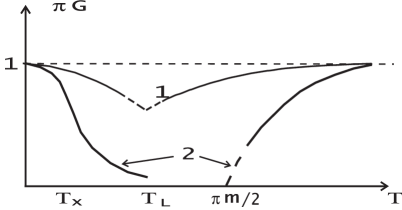
FIG. 3.: Schematic linear bias conductance $G$ vs. temperature near half-filling $\mu\ll T_{L}$: curve 1 for the weak interaction $m\ll T_{L}$, curve 2 for the strong one.

Calculation of above series with the uniform TLL correlator is equivalent to expanding the value $g=1/2$ into the leads. Following Luther and Emery [28] we map this bosonic Lagrangian onto the free massive fermion one [19, 20] with the density of Lagrangian

                                                                           

$${\cal L}_{F}=i\sum_{a=R,L=\pm}\psi^{+}_{a}(\partial_{t}\pm v_{c}\partial_{x})\psi_{a}-m\varphi(x)[e^{i(4k_{F}x+2Vt)}\psi^{+}_{L}(x,t)\psi_{R}(x,t)+h.c.]$$ (23)

                                                                           

Here $\psi_{R(L)}$ is right (left) chiral fermion field. The fermionized backscattering current $\hat{I}_{bsc}=2mi\int_{0}^{L}dx[exp\{i(4k_{F}x+2Vt)\}\psi^{+}_{L}(x,t)\psi_{R}(x,t)-h.c.]$ is the doubled backscattering current for the fermions [23] under doubled voltage. To find its average we just need to know the fermionic reflection coefficient $R$ as a function of dimensionless energy $\omega=\varepsilon/m$:

$$R(\omega)=\frac{\sin^{2}(\sqrt{\omega^{2}-1}\bar{t}_{L})}{(\omega^{2}-1)+\sin^{2}(\sqrt{\omega^{2}-1}\bar{t}_{L})}$$ (24)

where $\bar{t}_{L}\equiv m/T_{L}$ denotes the dimensionless traversal time. The analytical continuation is assumed for $|\omega|<1$. Since the chemical potential for the right/left chiral fermions is $\mu\pm V$, respectively, the total current can be expressed as

$$I={V\over\pi}-{m\sinh(V/T)\over\pi}\times$$ (26)

$$\hskip 14.22636pt\int d\omega\frac{R(\omega)}{\cosh((m\omega-\mu)/T)+\cosh(V/T)}$$

Only the leading term in $max(m,T_{L})/T$ of the right hand side of (26) is meaningful. Extracting it, we find the high-temperature asymptotics as following

$$I={V\over\pi}-{m\over\pi}\frac{\sinh(V/T)B(mt_{L})}{\cosh((\mu)/T)+\cosh(V/T)}$$ (28)

$$\hskip 8.53581ptB(x)\equiv\int d\omega\frac{\sin^{2}(\sqrt{\omega^{2}-1}x)}{(\omega^{2}-1)+\sin^{2}(\sqrt{\omega^{2}-1}x)}$$

where function $B(x)$ increases as $\pi x$ at small $x>0$ and approaches the constant $\simeq\pi$ at $x\gg 1$. Accuracy of this calculation of (26) may be written as a factor $1+O(max(m,T_{L})/max(T,V))$ to (14) if $|\mu|\ll max(T,V)$ or as $1+O([max(m,T_{L})/max(T,V)](max(T,V)/\mu)^{2}e^{|\mu|/T})$, otherwise. The high-temperature conductance (Fig.3)

$$G={1\over\pi}\left(1-{m\over T}\frac{B(m/T_{L})}{1+\cosh(\mu/T)}\right)$$ (29)

approaches zero at $T\approx m$ if the gap is large enough $m/T_{L}\gg 1$ and $|\mu|<m$. This asymptotics gives an adequate description of the whole high temperature region $T>m$ while a high energy value of $g$ was about 1/2. Then it complies with the high temperature conductance (16) we have found in the previous section. At others values of $g$ we would expect the conductance changing its behavior from (16) to (29) as $g$ is scaling with lowering the temperature. This crossover could result in a non- monotonous dependence of the conductance on the temperature, since at high energy $g>3/4$ we have seen that the conductance is increasing with decrease of the temperature.

2.Low energies $T,V<<T_{L}$ - To find a low energy model for our problem we have to integrate out all high energy modes. We will try to escape direct integration following Wiegmann’s effective way of constructing the Bethe-ansatz solvable models [29] for the Kondo problem and for the screening of a resonant level [29, 30]. First, let us substitute $\phi/\sqrt{2}$ instead of $\phi$ in (22). It makes fermions interacting inside the leads and non-interacting inside the wire. Their passage through the wire may be described with the one-electron $S$-matrix dependent on the electron momentum. The interaction between electrons in the leads with some two-particle $S$-matrix. Then the solution could be constructed if the proper commutation relations between the $S$-matrices are met. Being interested in the variation of energy less then $T_{L}$ around the Fermi level, one can simplify the solution keeping the one-particle $S$-matrix constant equal to its value on the Fermi level. It leads us to the problem of one impurity in the TLL.

For the weak backscattering, the Lagrangian of this problem can be written as

                                                                           

$$\int dx{\cal L}_{t}=\int dx{v_{F}\over 2}\{{1\over v_{F}^{2}}\left({{\partial_{t}\phi_{c}(t,x)}\over{\sqrt{4\pi}}}\right)^{2}-\left({{\partial_{x}\phi_{c}(t,x)}\over{\sqrt{4\pi}}}\right)^{2}\}-\frac{YT_{L}u}{\pi v_{F}}\cos(2Vt+\sqrt{2}\phi_{c}(t,0))$$ (30)

                                                                           

where we rescaled $\phi$ back and introduced a new energy cut-off parameter $YT_{L}$ with dimensionless constant $Y$ which will be specified later. Parameter $u$ is related to the weak reflection coefficient as:$u^{2}=v_{F}^{2}R(\mu/m)$. For the strong backscattering the tunneling Hamiltonian approach may be applied [31]. It was associated [7] to the dual representation using the field $\theta$ mutually conjugated to $\phi:\ [\theta_{\sigma}(x),\phi_{\sigma}(y)]=i2\pi sgn(x-y)$. The appropriate Lagrangian reads

                                                                           

$$\int dx{\cal L}_{t}=\int dx{v_{F}\over 2}\{{1\over v_{F}^{2}}\left({{\partial_{t}\theta_{c}(t,x)}\over{\sqrt{4\pi}}}\right)^{2}-\left({{\partial_{x}\theta_{c}(t,x)}\over{\sqrt{4\pi}}}\right)^{2}\}-\frac{YT_{L}u^{\prime}}{\pi v_{F}}\cos(Vt+\theta_{c}(t,0)/\sqrt{2})$$ (31)

                                                                           

with $u^{\prime 2}=v_{F}^{2}(1-R(\mu/m))$ proportional to the free massive fermion transmittance and the voltage multiplied by $g$ factor [32]. Both these Lagrangian are, indeed, equivalent [33] if interaction dependent relation between $u$ and $u^{\prime}$ is met [34, 32]. The above model (30) or(31) characterizes the point scatterer of any backscattering strength at low energy [7]. Although, the exact relation between $u$ or $u^{\prime}$ and the bare parameters of the scatterer remains unknown. Our problem is dually symmetrical to that of Kane and Fisher: suppression of the direct current in their problem equals suppression of the backscattering one in our case. This correspondence allows us to re-write their solution[34, 7] as follows:

$$I = {T_{x}\over\pi}Im\psi({1\over 2}+{T_{x}+iV\over\pi T})$$ (32)

$$I = {T_{x}\over\pi}\arctan(V/T_{x}),\ \ T=0$$ (33)

$$G = \frac{T_{x}}{\pi^{2}T}\psi^{\prime}({1\over 2}+{T_{x}\over\pi T})$$ (34)

where $\psi$ denotes the digamma function and satisfies: $\psi^{\prime}(1/2)=\pi^{2}/2,\ \psi^{\prime}(x)\propto 1/x,\ x\rightarrow\infty$, and a new energy scale $T_{x}$ [32] varies from $T_{x}=YT_{L}/\sqrt{4R}$ at the weak backscattering (30) to $T_{x}=YT_{L}(1-R)/\pi$ at the strong one (31).

Let us, first, compare this result with the perturbative one [18] of the previous section. The latter was derived making use of the long-time asymptotics for the correlator (19):

                                                                           

$$<e^{i\phi_{c}(x,t)}e^{-i\phi_{c}(y,0)}>=const\bigl{(}{\alpha T_{L}}\bigr{)}^{2g}\bigl{(}{{(\pi T/T_{L})^{2}}\over{sinh(\pi(t-i\alpha)T)sinh(\pi(-t+i\alpha)T)}}\bigr{)}F(x)F(y)$$ (35)

                                                                           

where $\alpha=1/E_{F}$ and $F$ was simplified in the previous section as: $F(x)=(x/L)^{gr}\prod_{\pm,m=1}^{\infty}(m\pm x/L)^{gr^{2m\pm 1}}\approx const^{\prime}\times[x(L-x)/L^{2}]^{gr}$ and $const^{\prime}=e^{\gamma(\infty)}$. One can see that substitution of this asymptotics in the whole formal series for the backscattering current discussed above implies transformation of the Lagrangian (22) into the one of (30) with the coefficient for the $\cos$-term: $e^{\gamma}\Gamma(1+r)mJ_{r+1/2}(E_{thr}t_{L})/\{\sqrt{\pi}(2E_{thr}t_{L})^{r+1/2}\}$ instead of $\frac{YT_{L}u}{\pi v_{F}}$ and another energy cut-off $T_{L}$. This model would be equivalent to that we constructed before in the weak perturbative regime if we can meet

$${Y\over\sin(\mu t_{L})}={2e^{-\gamma}\over\sqrt{\pi}\Gamma(1+r)}\frac{(2\mu t_{L})^{r-1/2}}{J_{r+1/2}(\mu t_{L})}$$ (36)

At zero $r$ it exactly specifies $Y$ as a constant on the order of 1. However, if $r\neq 0$ ($r=1/3$ for $g=1/2$ we assumed), $Y$ increases $\propto(\mu t_{L})^{r}$ at large $\mu t_{L}$. Moreover, there is a mismatching between the oscillating structures of $J_{r+1/2}(\mu t_{L})$ and $\sin(\mu t_{L})$ which cannot be naturally accounted for by a smooth variation of the energy cut-off, but sooner by a small deviation of the traversal time $t_{L}$ in the free electron reflection coefficient (26) from its bare value $L/v_{c}$ as $\mu$ changes. Such behavior results from penetration of the interaction inside the wire. It is described by the finite reflection coefficient $r$ in the inhomogeneous TLL model. The phenomenon is more important for $\mu\gg max(T_{L},m)$ when the electron propagation through the wire is not suppressed. In the opposite regime of small $|\mu|/T_{L}<1$ no interference structure is expected and $Y$ remains constant. Finally, under this choice (36) of $Y$ one can see that $T_{x}\gg T_{L}$. Therefore, the solution (33) coincides with the perturbative result (20, 21) that is $I-V/\pi\propto-V^{3}$ and $G-1/\pi\propto-T^{2}$.

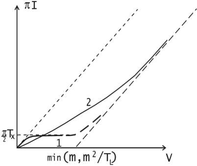
FIG. 4.: Schematic current $I$ vs. voltage $V$ near half-filling $\mu\ll T_{L}$: curve 1 is zero temperature dependence, curve 2 is the high temperature $T\gg T_{L}$ one, the dashed lines are the low voltage $I=V/\pi$ and high voltage asymptotics.

Turning to the case $m/T_{L}\geq 1$ we cannot use the perturbative expression (36) anymore: The perturbative series is not convergent due to a finite gap creation. Then above non-perturbative consideration is necessary. Application of the solution (33) in this case reveals a quite remarkable property of low energy transport through the Mott-Hubbard insulator. There is an exponentially small value of $T_{x}=(1-R(\mu/m))YT_{L}/\pi\propto T_{L}exp(-2m/T_{L})$ for $\mu\ll m$. Hence, the zero temperature current $I$ (Fig.4) is not suppressed for the voltage less than $T_{x}$ and saturates at $T_{x}/2$ value when $T_{x}<V<T_{L}$. Similarly, the conductance (Fig.3) displays a small decrease $\propto T^{2}$ below its zero temperature value $1/\pi$ with increase of $T$ for $T<T_{x}$ and approaches its exponentially small asymptotics $G=T_{x}/(4T)\propto exp(-2m/T_{L})T_{L}/T$ above $T_{x}<T<T_{L}$. As $|\mu|$ increases, the reflection coefficient $R(\mu/m)$ on the Fermi level goes down and $T_{x}$ exceeds $T_{L}$, finally, approaching its weak backscattering value $2T_{x}=YT_{L}/\sqrt{R(\mu/m)}$, where the perturbative consideration is applicable.

In summary, we studied transport through a 1D Mott-Hubbard insulator beyond perturbative approach. Assuming that $g=1/2$ near the half-filling in agreement with the Bethe ansatz solutions we mapped the problem onto the exactly solvable models and found current vs. voltage at high temperature $T>max(m,T_{L})$ and at low energy $T,V<T_{L}$. The solution of these models shows, in particularly, that the high-temperature transport through the Mott-Hubbard insulator is similar to the one through the band gap insulator at $g=1/2$. At low energies, however, there is always a regime where the transport remains non-suppressed in the absence of the impurity backscattering. For the strong interaction resulting in the opening of the large Mott-Hubbard gap, the transport through the wire is suppressed near the half-filling almost everywhere inside the gap except for an exponentially small low energy region $V,T<T_{L}exp(-m/T_{L})$.

V Acknowledgments

Most part of this work has been done in collaboration with Naoto Nagaosa when I was exercising hospitality of the University of Tokyo. I also acknowledge useful discussions with H. Fukuyama and S. Tarucha. The work was supported by the Center of Excellence at the Japanese Society for Promotion of Science and by the Swiss National Science Foundation.

$*$ On leave from A.F.Ioffe Physical Technical Institute, 194021, St. Petersburg, Russia

REFERENCES

- [1] S. Tarucha, T. Honda, and T. Saku, Solid State Commun. 94, 413 (1995).
- [2] A. Yacobi et al, Solid State Commun. 101, 77 (1996); Phys. Rev. Lett. 77, 4612 (1996).
- [3] L.P. Kouweenhoven et al, Phys. Rev. Lett. 65, 361 (1990).
- [4] D. L. Maslov and M. Stone, Phys. Rev. B 52, R5539 (1995).
- [5] V. V. Ponomarenko, Phys. Rev. B 52, R8666 (1995).
- [6] I. Safi and H. J. Schulz, Phys. Rev. B 52, R17040 (1995).
- [7] C. L. Kane and M. P. A. Fisher, Phys. Rev. Lett. 68, 1220 (1992); Phys. Rev. B 46, 15233 (1992); A. Furusaki and N. Nagaosa, Phys. Rev. B47, 4631 (1993).
- [8] M. Ogata and H. Fukuyama, Phys. Rev. Lett. 73, 468 (1994); W.Apel and T.M.Rice, Phys. Rev. B 26, 7063 (1982).
- [9] A. Kawabata, J. Phys. Soc. Jpn. 65, 30 (1996).
- [10] D. L. Maslov, Phys. Rev. B 52, R14368 (1995); A. Furusaki and N. Nagaosa, Phys. Rev. B54, R5239 (1996).
- [11] V.J. Emery, in Highly Conducting One-Dimensional Solid edited by J.T. Devreese (Plenum Press, New York, 1979), p.327.
- [12] H.J.Schulz, Phys. Rev Lett. 71, 1864 (1993).
- [13] T. Giamarchi, Phys. Rev B. 44, 2905 (1991).
- [14] F.D.M.Haldane, Phys. Rev. Lett. 47, 1840 (1981).
- [15] V. V. Ponomarenko, Phys. Rev. B 54, 10326 (1996); preprint cond-mat/9703085.
- [16] Y.Nazarov, A.Odintsov and D.Averin, Europhys. Lett 37, 213 (1997).
- [17] S. Tarucha, private communications.
- [18] V. V. Ponomarenko and N. Nagaosa, Phys. Rev. Lett. 79, 1714 (1997); A.A.Odintsov, Y.Tokura and S.Tarucha, Phys. Rev. B 56, R12729, (1997).
- [19] M.Mori, M. Ogata and H. Fukuyama, J. Phys. Soc. Jpn. 66, 3363 (1997).
- [20] O.A.Starykh and D. L. Maslov, Phys. Rev. Lett. 80, 1694 (1998).
- [21] V. V. Ponomarenko and N. Nagaosa, Phys. Rev. B 56, R12756, (1997).
- [22] V. V. Ponomarenko and N. Nagaosa, Phys. Rev. Lett. 81, 2304 (1998);
- [23] V. V. Ponomarenko and N. Nagaosa, preprint cond-mat/9709272, to appear in Solid State Commun. (1999).
- [24] A.B.Zamolodchikov and Al.B.Zamolodchikov, Ann. Phys. (N.Y.) 120, 253 (1979).
- [25] G.I. Japaridze, A.A. Nersesyan and P.B. Wiegmann, Nucl. Phys. B230, 511 (1984).
- [26] F.D.M. Haldane, Phys. Rev. Lett.45, 1358 (1980); H.J Schulz, Phys. Rev. Lett. 64, 2831 (1990).
- [27] M.J. Rice et al, Phys. Rev. Lett. 36, 432 (1976).
- [28] A.Luther and V.J. Emery, Phys. Rev. Lett. 33, 589 (1974).
- [29] A.M. Tsvelick and P.B. Wiegmann, Adv. Phys. 32, 453 (1983).
- [30] V. V. Ponomarenko, Phys. Rev. B 48, 5265 (1993).
- [31] V. V. Ponomarenko and N. Nagaosa, Phys. Rev. B 56, R12756, (1997) .
- [32] U. Weiss, Solid State Commun. 100, 281 (1996).
- [33] A. Schmid, Phys. Rev. Lett. 51, 1506 (1983).
- [34] P. Fendley et al, Phys. Rev. Lett. 74, 3005 (1995); Phys. Rev. B 52, 8934 (1995).