*

Abstract

The TB-LMTO-ASA method is reviewed and generalized to an accurate and robust TB-NMTO minimal-basis method, which solves Schrödinger’s equation to $N$th order in the energy expansion for an overlapping MT-potential, and which may include any degree of downfolding. For $N=1,$ the simple TB-LMTO-ASA formalism is preserved. For a discrete energy mesh, the NMTO basis set may be given as: $\chi^{\left(N\right)}\left(\mathbf{r}\right)=\sum_{n}\phi\left(\varepsilon_{n},\mathbf{r}\right)L_{n}^{\left(N\right)}$ in terms of kinked partial waves, $\phi\left(\varepsilon,\mathbf{r}\right),$ evaluated on the mesh, $\varepsilon_{0},...,\varepsilon_{N}.$ This basis solves Schrödinger’s equation for the MT-potential to within an error $\propto\left(\varepsilon-\varepsilon_{0}\right)...\left(\varepsilon-\varepsilon_{N}\right).$ The Lagrange matrix-coefficients, $L_{n}^{\left(N\right)},$ as well as the Hamiltonian and overlap matrices for the NMTO set, have simple expressions in terms of energy derivatives on the mesh of the Green matrix, defined as the inverse of the screened KKR matrix. The variationally determined single-electron energies have errors $\propto$ $\left(\varepsilon-\varepsilon_{0}\right)^{2}...\left(\varepsilon-\varepsilon_{N}\right)^{2}.$ A method for obtaining orthonormal NMTO sets is given and several applications are presented.

1 Overview

Muffin-tin orbitals (MTOs) have been used for a long time in ab initio calculations of the electronic structure of condensed matter. Over the years, several MTO-based methods have been devised and further developed. The ultimate aim is to find a generally applicable electronic-structure method which is accurate and robust, as well as intelligible.

In order to be intelligible, such a method must employ a small, single-electron basis of atom-centered, short-ranged orbitals. Moreover, the single-electron Hamiltonian must have a simple, analytical form, which relates to a two-center, orthogonal, tight-binding (TB) Hamiltonian.

In this sense, the conventional linear muffin-tin-orbitals method in the atomic-spheres approximation (LMTO-ASA) [1, 2] is intelligible, because the orbital may be expressed as:

$$\chi_{RL}\left(\mathbf{r}_{R}\right)\;=\;\phi_{RL}\left(\mathbf{r}_{R}\right)+\sum_{R^{\prime}L^{\prime}}\dot{\phi}_{R^{\prime}L^{\prime}}\left(\mathbf{r}_{R^{\prime}}\right)\left(H_{R^{\prime}L^{\prime},RL}-\varepsilon_{\nu}\delta_{R^{\prime}R}\delta_{L^{\prime}L}\right).$$ (1)

Here, $\phi_{RL}\left(\mathbf{r}_{R}\right)$ is the solution, $\varphi_{Rl}\left(\varepsilon_{\nu},r_{R}\right)Y_{lm}\left(\mathbf{\hat{r}}_{R}\right),$ at a chosen energy, $\varepsilon_{\nu},$ of Schrödinger’s differential equation inside the atomic sphere at site $R$ for the single-particle potential, $\sum_{R}v_{R}\left(r_{R}\right)\,,$ assumed to be spherically symmetric inside that sphere. Moreover, $\mathbf{r}_{R}\equiv\mathbf{r-R}$ and $L\equiv lm.\;$The function $\varphi_{Rl}\left(\varepsilon,r\right)$ thus satisfies the one-dimensional, radial Schrödinger equation

$$\frac{\partial^{2}}{\partial r^{2}}r\varphi_{Rl}\left(\varepsilon,r\right)=-\left[\varepsilon-v_{R}\left(r\right)-\frac{l\left(l+1\right)}{r^{2}}\right]r\varphi_{Rl}\left(\varepsilon,r\right).$$ (2)

In (1), $\dot{\phi}_{RL}\left(\mathbf{r}\right)$ are the energy-derivative functions, $\left.\partial\varphi_{Rl}\left(\varepsilon,r\right)/\partial\varepsilon\right|_{\varepsilon_{\nu}}Y_{lm}\left(\mathbf{\hat{r}}\right).$ The radial functions, $\varphi$ and $\dot{\varphi},$ and also the potential, $v,$ are truncated outside their own atomic sphere of radius $s,$ and the matrix, $H,$ is constructed in such a way that the LMTO is continuous and differentiable in all space. Equation (1) therefore expresses the LMTO at site $R$ and (pseudo) angular momentum $L$ as the solution of Schrödinger’s equation at that site, with that angular momentum, and at the chosen energy, plus a ’smoothing cloud’ of energy-derivative functions, centered mainly at the neighboring sites, and having around these, all possible angular momenta.

That a set of energy-independent orbitals must have the form (1) in order to constitute a basis for the solutions $\Psi_{i}\left(\mathbf{r}\right)$ –with energies $\varepsilon_{i}$ in the neighborhood of $\varepsilon_{\nu}$– of Schrödinger’s equation for the entire system, is intuitively obvious, because the corresponding linear combinations, $\sum_{RL}\chi_{RL}\left(\mathbf{r}_{R}\right)\,c_{RL,i},$ will be those which locally, inside each atomic sphere and for each angular momentum, have the right amount of $\dot{\varphi}$ –provided mainly by the tails of the neighboring orbitals– added onto the central orbital’s $\varphi.$ Since by construction each $\varphi_{Rl}\left(\varepsilon,r\right)$ is the correct solution, this right amount is of course $\varepsilon_{i}-\varepsilon_{\nu}.$ In math: since definitions can be made such that the expansion matrix $H_{R^{\prime}L^{\prime},RL}$ is Hermitian, its eigenvectors are the coefficients of the proper linear combinations, and its eigenvalues are the energies:

$$\sum_{RL}\chi_{RL}\left(\mathbf{r}_{R}\right)\,c_{RL,i}\; = \;\sum_{RL}\left[\phi_{RL}\left(\mathbf{r}_{R}\right)+\left(\varepsilon_{i}-\varepsilon_{\nu}\right)\dot{\phi}_{RL}\left(\mathbf{r}_{R}\right)\right]c_{RL,i}$$ (3)

$$\approx \;\sum_{RL}\phi_{RL}\left(\varepsilon_{i},\mathbf{r}_{R}\right)c_{RL,i}\;=\;\Psi_{i}\left(\mathbf{r}\right).$$

Hence, $H$ is a 1st-order Hamiltonian, delivering energies and wave functions with errors proportional to $\left(\varepsilon_{i}-\varepsilon_{\nu}\right)^{2},$ to leading order.

First-order energies seldom suffice, and in the conventional LMTO-ASA method use is made of the variational principle for the Hamiltonian,

$$\mathcal{H\;}\equiv\;-\nabla^{2}\;+\;\sum\nolimits_{R}v_{R}\left(r_{R}\right)\,,$$ (4)

so that errors of order $\left(\varepsilon_{i}-\varepsilon_{\nu}\right)^{2}$ in the basis set merely give rise to errors of order $\left(\varepsilon_{i}-\varepsilon_{\nu}\right)^{4}$ in the energies. With that approach, the energies and eigenvectors are obtained as solutions of the generalized eigenvalue problem:

$$\sum_{RL}\left[\left\langle\chi_{R^{\prime}L^{\prime}}\left|\mathcal{H}-\varepsilon_{\nu}\right|\chi_{RL}\right\rangle-\left(\varepsilon_{i}-\varepsilon_{\nu}\right)\left\langle\chi_{R^{\prime}L^{\prime}}\mid\chi_{RL}\right\rangle\right]c_{RL,i}=0,$$ (5)

for all $R^{\prime}L^{\prime}.$ If we now insert (1) in (5), we see that the Hamiltonian and overlap matrices are expressed in terms of the 1st-order Hamiltonian, $H,$ plus two diagonal matrices with the respective elements

$$\left\langle\phi_{RL}\mid\dot{\phi}_{RL}\right\rangle=\textstyle{\int_{0}^{s}}\varphi_{Rl}\left(r\right)\dot{\varphi}_{Rl}\left(r\right)r^{2}dr,\;\;\;\left\langle\dot{\phi}_{RL}\mid\dot{\phi}_{RL}\right\rangle=\int_{0}^{s}\dot{\varphi}_{Rl}\left(r\right)^{2}r^{2}dr.$$

These matrices are diagonal by virtue of the ASA, which approximates integrals over space by the sum of integrals over atomic spheres. If each partial wave is normalized to unity in its sphere: $\int_{0}^{s}\varphi_{Rl}\left(r\right)^{2}r^{2}dr=1,$ then $\left\langle\phi\mid\phi\right\rangle$ is the unit matrix in the ASA, and the Hamiltonian and overlap matrices entering (5) take the simple forms:

$$\left\langle\chi\left|\mathcal{H}-\varepsilon_{\nu}\right|\chi\right\rangle\; = \;\left(H-\varepsilon_{\nu}\right)\left[1+\left\langle\phi\mid\dot{\phi}\right\rangle\left(H-\varepsilon_{\nu}\right)\right]$$ (6)

$$\left\langle\chi\mid\chi\right\rangle\; = \;\left[1+\left(H-\varepsilon_{\nu}\right)\left\langle\dot{\phi}\mid\phi\right\rangle\right]\left[1+\left\langle\phi\mid\dot{\phi}\right\rangle\left(H-\varepsilon_{\nu}\right)\right]$$

$$\quad\quad\quad+\;\left(H-\varepsilon_{\nu}\right)\left[\left\langle\dot{\phi}\mid\dot{\phi}\right\rangle-\left\langle\phi\mid\dot{\phi}\right\rangle^{2}\right]\left(H-\varepsilon_{\nu}\right).$$

Here and in the following we use a vector-matrix notation according to which, for example $\chi_{RL}\left(\mathbf{r}_{R}\right)$ and $\chi_{RL}\left(\mathbf{r}_{R}\right)^{\ast}$ are considered components of respectively a row-vector, $\chi\left(\mathbf{r}\right),$ and a column-vector, $\chi\left(\mathbf{r}\right)^{\dagger}.$ The eigenvector, $c_{i},$ is a column vector with components $c_{RL,i}.$ Moreover, $1$ is the unit matrix, $\varepsilon_{\nu}$ is a diagonal matrix, and $H$ is a Hermitian matrix. Vectors and diagonal matrices are denoted by lower-case Latin and Greek characters, and matrices by upper-case Latin characters. Exceptions to this rule are: $Y\left(\mathbf{\hat{r}}\right),$ the vector of spherical harmonics, the site and angular-momentum indices (subscripts) $R,\,L,\,I,$ and $A,$ and the orders (superscripts) $L,\,M,$ and $N.$ Operators are given in calligraphic, like $\mathcal{H},$ and an omitted energy argument means that $\varepsilon=\varepsilon_{\nu}.$

With the $\phi\left(\mathbf{r}\right)$’s being orthonormal in the ASA, the LMTO overlap matrix in (6) is seen to factorize to 1st order, and it is therefore simple to transform to a set of nearly orthonormal LMTOs:

$$\hat{\chi}\left(\mathbf{r}\right)\; = \;\chi\left(\mathbf{r}\right)\left[1+\left\langle\phi\mid\dot{\phi}\right\rangle\left(H-\varepsilon_{\nu}\right)\right]^{-1}$$ (7)

$$\left\langle\hat{\chi}\left|\mathcal{H}-\varepsilon_{\nu}\right|\hat{\chi}\right\rangle\; \equiv \;\hat{H}-\varepsilon_{\nu}\;=\;\left[1+\left(H-\varepsilon_{\nu}\right)\left\langle\dot{\phi}\mid\phi\right\rangle\right]^{-1}\left(H-\varepsilon_{\nu}\right)$$

$$= \;H-\varepsilon_{\nu}\;-\;\left(H-\varepsilon_{\nu}\right)\left\langle\dot{\phi}\mid\phi\right\rangle\left(H-\varepsilon_{\nu}\right)\;+\;...$$

$$\left\langle\hat{\chi}\mid\hat{\chi}\right\rangle\; = \;1\;+\;\left(\hat{H}-\varepsilon_{\nu}\right)\left\langle\overset{.}{\hat{\phi}}\mid\overset{.}{\hat{\phi}}\right\rangle\left(\hat{H}-\varepsilon_{\nu}\right)$$

$$\overset{.}{\hat{\phi}}\left(\mathbf{r}\right)\; \equiv \;\dot{\phi}\left(\mathbf{r}\right)\;-\;\phi\left(\mathbf{r}\right)\left\langle\phi\mid\dot{\phi}\right\rangle.$$

Here, the energy-derivative function, $\overset{.}{\hat{\phi}}\left(\mathbf{r}\right),$ equals $\dot{\phi}\left(\mathbf{r}\right),$ orthogonalized to $\phi\left(\mathbf{r}\right).$ Finally, we may transform to a set of orthonormal LMTOs:

$$\check{\chi}\left(\mathbf{r}\right)\;=\;\hat{\chi}\left(\mathbf{r}\right)\left[1+\left(\hat{H}-\varepsilon_{\nu}\right)\left\langle\overset{.}{\hat{\phi}}\mid\overset{.}{\hat{\phi}}\right\rangle\left(\hat{H}-\varepsilon_{\nu}\right)\right]^{-1/2}\;=$$ (8)

$$\quad\quad\quad\quad\quad\quad\quad\quad\quad\quad\hat{\chi}\left(\mathbf{r}\right)\left[1-\frac{1}{2}\left(\hat{H}-\varepsilon_{\nu}\right)\left\langle\overset{.}{\hat{\phi}}\mid\overset{.}{\hat{\phi}}\right\rangle\left(\hat{H}-\varepsilon_{\nu}\right)+..\right]$$

$$\left\langle\check{\chi}\left|\mathcal{H}-\varepsilon_{\nu}\right|\check{\chi}\right\rangle\;\equiv\;\check{H}-\varepsilon_{\nu}\;=\;\hat{H}-\varepsilon_{\nu}-$$

$$\frac{1}{2}\left(\hat{H}-\varepsilon_{\nu}\right)\left\langle\overset{.}{\hat{\phi}}\mid\overset{.}{\hat{\phi}}\right\rangle\left(\hat{H}-\varepsilon_{\nu}\right)^{2}-\frac{1}{2}\left(\hat{H}-\varepsilon_{\nu}\right)^{2}\left\langle\overset{.}{\hat{\phi}}\mid\overset{.}{\hat{\phi}}\right\rangle\left(\hat{H}-\varepsilon_{\nu}\right)+..$$

We thus realize that of the Hamiltonians considered, $H$ is of 1st, $\hat{H}$ is of 2nd, and $\check{H}$ is of 3rd order. As the order increases, and the energy window –inside which the eigenvalues of the Hamiltonian are useful as single-electron energies– widens, the real-space range of the Hamiltonian increases. For real-space calculations [3, 4, 5, 6, 7], it is therefore important to be able to express a higher-order Hamiltonian as a power series in a lower-order Hamiltonian like in (7) and (8), because such a series may be truncated when the energy window is sufficiently wide.

The energy-derivative of the radial function $\varphi\left(\varepsilon,r\right)$ depends on the energy derivative of its normalization. If we choose to normalize according to: $\int_{0}^{s}\hat{\varphi}\left(\varepsilon,r\right)^{2}r^{2}dr=1,$ then it follows that $\int_{0}^{s}\hat{\varphi}\left(r\right)\overset{.}{\hat{\varphi}}\left(r\right)r^{2}dr=0.$ Choosing another energy-dependent normalization: $\varphi\left(\varepsilon,r\right)\equiv\hat{\varphi}\left(\varepsilon,r\right)\left[1+\left(\varepsilon-\varepsilon_{\nu}\right)o\right],$ specified by a constant $o,$ then we see that: $\dot{\varphi}\left(r\right)=\overset{.}{\hat{\varphi}}\left(r\right)+\varphi\left(r\right)o.$ Changing the energy derivative of the normalization thus adds some $\varphi\left(r\right)$ to $\overset{.}{\hat{\varphi}}\left(r\right)$ and thereby changes the shape of the ’tail function’ $\dot{\varphi}\left(r\right).$ Since all LMTOs (1) should remain smooth upon this change, also $H$ must change, and so must all LMTOs in the set. The diagonal matrix $\left\langle\phi\mid\dot{\phi}\right\rangle,$ whose elements are the radial overlap integrals: $o=\int_{0}^{s}\varphi\left(r\right)\dot{\varphi}\left(r\right)r^{2}dr,$ thus determines the LMTO representation, and the first and the last equations (7) specify the linear transformation between representations. Values of the diagonal matrix $\left\langle\phi\mid\dot{\phi}\right\rangle$ exist, which yield short range for the 1st-order Hamiltonian $H$ and, hence, for the LMTO set (1). Such an $H$ is therefore a two-center TB Hamiltonian and such an LMTO set is a first-principles TB basis.

In order to obtain an explicit expression for $H,$ one needs to find the spherical-harmonics expansions about the various site for a set of smooth MTO envelope functions. For a MT-potential, which is flat in the interstitial, the envelope functions are wave-equation solutions with pure spherical-harmonics character near the sites. Consistent with the idea behind the ASA –to use ’space-filling spheres’– is the use of envelope functions with fixed energy, specifically zero, which is a reasonable approximation for the kinetic energy between the atoms for a valence state. The envelope functions in the ASA are thus screened multipole potentials, with the screening specified by a diagonal matrix of screening constants, $\alpha_{Rl},$ related to the radial overlaps $o_{Rl}$. The expansion of a bare multipole potential at site $R$ about a different site $R^{\prime}$ is well known:

$$\frac{Y_{L}\left(\mathbf{\hat{r}}_{R}\right)}{r_{R}^{l+1}}\sim\sum_{R^{\prime}L^{\prime}}r_{R^{\prime}}^{l^{\prime}}Y_{L^{\prime}}\left(\mathbf{\hat{r}}_{R^{\prime}}\right)\,\frac{Y_{l^{\prime\prime}m^{\prime\prime}}\left(\widehat{\mathbf{R}^{\prime}\mathbf{-R}}\right)}{\left|\mathbf{R}^{\prime}\mathbf{-R}\right|^{l^{\prime\prime}+1}}\sim\sum_{R^{\prime}L^{\prime}}\,r_{R^{\prime}}^{l^{\prime}}Y_{L^{\prime}}\left(\mathbf{\hat{r}}_{R^{\prime}}\right)\,\mathsf{S}_{R^{\prime}L^{\prime},RL}^{0}\,.$$

Here, $l^{\prime\prime}\equiv l^{\prime}+l$ and $m^{\prime\prime}\equiv m^{\prime}-m.$ With suitable normalizations, the bare structure matrix, $\mathsf{S}^{0},$ can be made Hermitian. The screened structure matrix is now related to the bare one through a Dyson equation:

$$\left(\mathsf{S}^{\alpha}\right)^{-1}\;\mathsf{=\;}\left(\mathsf{S}^{0}\right)^{-1}-\,\alpha,$$ (9)

which may be solved by inversion of the matrix $\mathsf{S}^{0}-\alpha^{-1}.$ This inversion may be performed in real space, that is in $\mathbf{R}$- rather than in $\mathbf{k}$-representation, provided that the screening constants take values known from experience to give a short-ranged $\mathsf{S}^{\alpha}.$

In the end, it turns out that all ingredients to the LMTO Hamiltonian and overlap integrals, $H,$ $\left\langle\phi\mid\dot{\phi}\right\rangle,$ and $\left\langle\dot{\phi}\mid\dot{\phi}\right\rangle,$ may be obtained from the screened Korringa-Kohn-Rostoker (KKR) matrix in the ASA:

$$\mathsf{K}_{R^{\prime}L^{\prime},RL}^{\alpha}\left(\varepsilon\right)\equiv\mathsf{p}_{Rl}^{\alpha}\left(\varepsilon\right)\delta_{R^{\prime}R}\delta_{L^{\prime}L}-\mathsf{S}_{R^{\prime}L^{\prime},RL}^{\alpha}.$$ (10)

Here, $\mathsf{p}^{0}\left(\varepsilon\right)$ is a diagonal matrix of potential functions obtained from the radial logarithmic derivative functions, $\partial\left\{\varphi\left(\varepsilon,s\right)\right\}\equiv\partial\ln\left|\varphi\left(\varepsilon,r\right)\right|\left/\partial\ln r\right|_{s},$ evaluated at the MT-radius, and $\mathsf{p}^{\alpha}\left(\varepsilon\right)$ is related to $\mathsf{p}^{0}\left(\varepsilon\right)$ via the diagonal version of Equation (9). The results are:

$$H\;=\;\varepsilon_{\nu}-K\;=\;\varepsilon_{\nu}-\mathsf{p\dot{p}}^{-1}+\mathsf{\dot{p}}^{-\frac{1}{2}}\mathsf{S}\,\mathsf{\dot{p}}^{-\frac{1}{2}}\;\equiv\;\mathsf{c}+\mathsf{d}^{\frac{1}{2}}\mathsf{S}\,\mathsf{d}^{\frac{1}{2}},$$

$$\left\langle\phi\mid\dot{\phi}\right\rangle=\frac{\ddot{K}}{2!}=\frac{1}{2!}\frac{\mathsf{\ddot{p}}}{\mathsf{\dot{p}}}\,,\quad\quad\left\langle\dot{\phi}\mid\dot{\phi}\right\rangle=\frac{\dddot{K}}{3!}=\frac{1}{3!}\frac{\mathsf{\dddot{p}}}{\mathsf{\dot{p}}}\,,$$ (11)

expressed in terms of the KKR matrix, renormalized to have $\dot{K}=1:$

$$K\left(\varepsilon\right)\;\equiv\;\mathsf{\dot{K}}^{-\frac{1}{2}}\,\mathsf{K}\left(\varepsilon\right)\mathsf{\dot{K}}^{-\frac{1}{2}}\;=\;\mathsf{p}\left(\varepsilon\right)\mathsf{\dot{p}}^{-1}-\mathsf{\dot{p}}^{-\frac{1}{2}}\mathsf{S}\,\mathsf{\dot{p}}^{-\frac{1}{2}}.$$ (12)

This corresponds to the partial-wave normalization: $\int_{0}^{s}\varphi\left(r\right)^{2}r^{2}dr=1,$ and $K\left(\varepsilon\right)$ is what in the 2nd-generation method [1, 2] is denoted $-h\left(\varepsilon\right),$ but since the current notation identifies matrices by capitals, we have changed. The LMTO Hamiltonian and overlap matrices are thus expressed solely in terms of the structure matrix $\mathsf{S}$ and the potential functions $\mathsf{p}\left(\varepsilon\right),$ specifically the diagonal matrices $\mathsf{p},$ $\mathsf{\dot{p}},\;\mathsf{\ddot{p}},\mathrm{\;}$and$\;\mathsf{\dddot{p}}$. It may be realized that the nearly-orthonormal representation is generated if the diagonal screening matrix in (9) is set to the value $\gamma,$ which makes $\mathsf{\ddot{p}}^{\gamma}$ vanish.

For calculations [8, 9, 10] which employ the coherent-potential approximation (CPA) to treat substitutional disorder, it is important to be able to perform screening transformations of the Green matrix:

$$\mathsf{G}^{\alpha}\left(z\right)\equiv\mathsf{K}^{\alpha}\left(z\right)^{-1}=\left[\mathsf{p}^{\alpha}\left(z\right)-\mathsf{S}^{\alpha}\right]^{-1},$$ (13)

also called the resolvent, or the scattering path operator in multiple scattering theory [11]. In the 2nd generation MTO formalism, $\mathsf{G}^{a}\left(\varepsilon\right)$ was denoted $g^{\alpha}\left(\varepsilon\right).$ This screening transformation is:

$$\mathsf{G}^{\beta}\left(z\right)=\left(\beta-\alpha\right)\frac{\mathsf{p}^{\alpha}\left(z\right)}{\mathsf{p}^{\beta}\left(z\right)}+\frac{\mathsf{p}^{\alpha}\left(z\right)}{\mathsf{p}^{\beta}\left(z\right)}\mathsf{G}^{\alpha}\left(z\right)\frac{\mathsf{p}^{\alpha}\left(z\right)}{\mathsf{p}^{\beta}\left(z\right)},$$ (14)

and is seen to involve no matrix multiplications, but merely energy-dependent rescaling of matrix elements. As a transformation between the nearly orthonormal, $\beta\mathrm{=}\gamma,$ and the short-ranged TB-representation, Eq. (14) has been useful also in Green-function calculations for extended defects, surfaces, and interfaces [8, 10, 12, 13, 14]. However, calculations which start out from the unperturbed Green matrices most natural for the problem –namely those obtained from LMTO band-structure calculations in the nearly orthonormal representation for the bulk systems– have usually been limited to 2nd-order in $z-\varepsilon_{\nu}$, because $\mathsf{p}^{\gamma}\left(z\right)$ is linear to this order, and because attempts to use 3rd-order expressions for $\mathsf{p}^{\gamma}\left(z\right)$ employing the potential parameter $\mathsf{\dddot{p}}^{\gamma}=3!\,\mathsf{\dot{p}}^{\gamma}\left\langle\overset{.}{\hat{\phi}}\mid\overset{.}{\hat{\phi}}\right\rangle,$ induced false poles in the Green matrix.

What is not intelligible in the TB-LMTO-ASA method is that the LMTO expansion (1) must include all $L^{\prime}$’s until convergence is reached throughout each sphere, and all $R^{\prime}$’s until space is covered with spheres. This means that the LMTO-ASA basis is minimal –at most– for elemental, closely packed transition metals, the case for which it was in fact invented [15]. The supreme computational efficiency of the method soon made self-consistent density-functional [16] calculations possible, and not only for elemental transition metals, but also for compounds. In order to treat open structures such as diamond, empty spheres were introduced as a device for describing the repulsive potentials in the interstices [17]. All of this then, led to misinterpretations of the wave-function related output of such calculations in terms of the components of the one-center expansions (1), typically the numbers of $s,$ $p,$ and $d$ electrons on the various atoms (including in the empty spheres!) and the charge transfers between them. Absurd statements to the effect that CsCl is basically a neutral compound with the Cs electron having a bit of $s$-, more $p$-, quite some $d$-, and a bit of $f$-character were not uncommon. Many practitioners of the ASA method did not realize that the role of the MT-spheres is to describe the input potential, rather than the output wave-functions. For the latter, the one-center expansions truncated outside the spheres constitute merely a decomposition which is used in the code for selfconsistent calculations. The strange Cs electron is therefore little more than the expansion about the Cs site of the tails of the neighboring Cl $p$ electrons spilling into the Cs sphere. That latter MT-sphere must of course be chosen to have about the same size as that of Cl, because only then is the shape of the Cs⁺Cl^- potential in the bi-partitioned structure well described.

Now, the so-called high partial waves –they are those which are shaped like $r^{l}$ in the outer part of the sphere where the potential flattens out– do enter the LMTO expansion (1), but not the eigenvalue problem (5) or the equivalent KKR equation:

$$K\left(\varepsilon_{i}\right)c_{i}=0,$$ (15)

because they are part of the MTO envelope functions. This property of having the high-$l$ limit correct is a strength of the MTO method, not shared by for instance Gaussian orbitals, which are solutions of (2) for a parabolic potential. There are, however, also other partial waves –like the Cs $s$-waves, $d$-waves in non-transition metal atoms, $f$-waves in transition-metal atoms, $s$-waves in oxygen and fluorine, and in positive alkaline ions, and all partial waves in empty spheres– which for the problem at hand are judged to be inactive and should therefore not have corresponding LMTOs in the basis. In order to get rid of such inactive LMTOs, one must first –by means of (9) or (14)– transform to a representation in which the inactive partial waves appear only in the ’tails’ (second term of (1)) of the remaining LMTOs; only thereafter, the inactive LMTOs can be deleted. This down-folding procedure works for the LMTO-ASA method, but it messes up the connection between the LMTO Hamiltonian (6)-(12) and the KKR Green-function formalisms (11)-(15), and it is not as efficient as one would have liked it to be [2]. E.g., the Si valence band cannot be described with an $sp$ LMTO basis set derived by down-folding of the Si $d$- as well as all empty-sphere partial waves [18].

The basic reason for these failures is that the ASA envelopes are chosen to be independent of energy –in order to avoid energy dependence of the structure matrix– because this is what forces us to carry out explicitly the integrals involving all partial waves in all spheres throughout space. What should be done is to include all inactive waves, $\varphi_{I}\left(\varepsilon,r\right),$ in energy-dependent MTO-envelopes, and then to linearize these MTOs to form LMTOs. This has been achieved with the development of the LMTO method of the 3rd-generation [19, 20], and will be dealt with in the present paper. The reason why energy linearization still works in a window of useful width, now that the energy dependence is kept throughout space, is due to the screening of the wave-equation solutions used as envelope functions [21].

As an extreme example, it was demonstrated in Fig. 7 of Ref. [20] –and we shall present further results in Fig. 11 below– how with this method one may pick the orbital of one band, with a particular local symmetry and energy range, out of a complex of overlapping bands. This goes beyond the construction of a Wannier function and has relevance for the treatment of correlated electrons in narrow bands [22, 23]. Another example to be treated in the present paper is the valence and low-lying conduction-band structure of GaAs calculated with the minimal Ga $spd$ As $sp$ basis [24]. Other examples, not treated in this paper, concern the calculation of chemical indicators, such as the crystal-orbital-overlap-projected densities of states (COOPs) [25] for describing chemical pair bonding. These indicators were originally developed for the empirical Hückel method where all parameters have been standardized. When one tries to take this over to an ab initio method, one immediately gets confronted with the problems of representation. For instance, COOPs will vanish in a basis of orthonormal orbitals. Therefore, the COOPs first had to be substituted by COHPs, which are Hamiltonian- rather than overlap projections, but still, the LMTO-ASA method often gave strange results –for the above mentioned reasons [26]. What one has to do is –through downfolding– to chose the chemically-correct LMTO Hilbert space and –through screening– choose the chemically correct axes (orbitals) in this space. Only with such orbitals, does it make sense to compute indicators [27, 28].

A current criterion for an electronic-structure method to be accurate and robust is that it can be used in ab initio density-functional molecular-dynamics (DF-MD) calculations [29]. According to this criterion, hardly any existing LMTO method –and the LMTO-ASA least of all– is accurate and robust.

Most LMTO calculations include non-ASA corrections to the Hamiltonian and overlap matrices, such as the combined correction for the neglected integrals over the interstitial region and the neglected high partial waves. This brings in the first energy derivative of the structure matrix, $\mathsf{\dot{S}},$ in a way which makes the formalism clumsy [2]. The code [30] for the 2nd-generation LMTO method is useful [31] and quite accurate for calculating energy bands, because it includes downfolding in addition to the combined correction, as well as an automatic way of dividing space into MT-spheres, but the underlying formalism is complicated.

There certainly are LMTO methods sufficiently accurate to provide structural energies and forces within density-functional theory [32, 33, 34, 35, 36, 37, 38, 39, 40], but their basis functions are defined with respect to MT-potentials which do not overlap. As a consequence, in order to describe adequately the correspondingly large interstitial region, these LMTO sets must include extra degrees of freedom, such as LMTOs centered at interstitial sites and LMTOs with more than one radial quantum number. The latter include LMTOs with tails of different kinetic energies (multiple kappa -sets) and LMTOs for semi-core states. Moreover, these methods usually do not employ short-ranged representations. Finally, since a non-overlapping MT potential is a poor approximation to the self-consistent potential, these methods are forced to include the matrix elements of the full potential. Existing full-potential methods are thus set up to provide final, numerical results at relatively low cost, but since they are complicated, they have sofar lacked the robustness needed for DF-MD, and their formalisms provide little insight to the physics and chemistry of the problem.

One of the early full-potential MTO methods did fold down extra orbitals and furthermore contained a scheme by which the matrix elements of the full potential could be efficiently approximated by integrals in overlapping spheres [38]. The formalism however remained complicated, and the method apparently never took off. A decade later, it was shown [21, 20] that the MT-potential, which defines the MTOs –and to which the Hamiltonian (4) refers– may in fact have some overlap: If one solves the exact KKR equations [41] with phase shifts calculated for MT-wells which overlap, then the resulting wave function is the one for the superposition of these MT-wells, plus an error of 2nd order in the potential-overlap. This proof will be repeated in Eq. (2.1) of the present paper, and in Figs. 14 and 13 we shall supplement the demonstration in Ref. [20] that this may be exploited to make the kind of extra LMTOs mentioned above superfluous, provided that the MTO-envelopes have the proper energy dependence, that is, provided that 3rd generation LMTOs are used. Presently we can handle MT-potentials with up to $\sim$60% radial overlap $\left(s_{R}+s_{R^{\prime}}<1.6\left|\mathbf{R-R}^{\prime}\right|\right)$, and it seems as if such potentials, with the MT-wells centered exclusively on the atoms, are sufficiently realistic that we only need the minimal LMTO set defined therefrom [20, 42]. It may even be that such fat MT-potentials, without full-potential corrections to the Hamiltonian matrix, will yield output charge densities which, when used in connection with the Hohenberg-Kohn variational principle for the total energy [16], will yield good structural energies [43]. Hence, we are getting rid of one of the major obstacles to LMTO DF-MD calculations, the empty spheres.

Soon after the development of the TB-LMTO-ASA method, it was realized [44] that the full charge density produced with this method –for cases where atomic and interstitial MT-spheres fill space well– is so accurate, that it should suffice for the calculation of total energies, provided that this charge density is used in connection with a variational principle. However, it took ten years before the first successful implementation was published [45]. The problem is as follows: The charge density, $\rho\left(\mathbf{r}\right)=\sum_{i}^{occ}\left|\Psi_{i}\left(\mathbf{r}\right)\right|,$ is most simply obtained in the form of one-center expansions:

$$\rho\left(\mathbf{r}\right)=\sum_{R}\sum_{LL^{\prime}}\int_{occ}\phi_{RL}\left(z,\mathbf{r}_{R}\right)\,{\rm Im}G_{RL,RL^{\prime}}\left(z\right)\,\phi_{RL^{\prime}}\left(z,\mathbf{r}_{R}\right)^{\ast}\frac{dz}{\pi},$$ (16)

where $G\left(z\right)\equiv K\left(z\right)^{-1},$ as can be seen from (1) and (3), but these expansions have terribly bad $L$-convergence in the region between the atoms and cannot even be used to plot the charge-density in that region. That was made possible by the transformation to a short-ranged representation, because one could now use:

$$\rho\left(\mathbf{r}\right)=\sum_{RL}\sum_{R^{\prime}L^{\prime}}\chi_{RL}\left(\mathbf{r}_{R}\right)\,\left[\int_{occ}{\rm Im}G_{RL,R^{\prime}L^{\prime}}\left(z\right)\,\frac{dz}{\pi}\right]\,\chi_{R^{\prime}L^{\prime}}\left(\mathbf{r}_{R^{\prime}}\right)^{\ast},$$ (17)

where the $L$-sums only run over active values, and where the double-sum over sites converges fast. Nevertheless, to compute a value of $\chi_{RL}\left(\mathbf{r}\right)$ with $\mathbf{r}$ far away from a site, one must evaluate the LMTO envelope function, which is a superposition of the bare ones, $Y_{L}\left(\mathbf{\hat{r}}_{R}\right)/r_{R}^{l+1},$ and this means that (17) actually contains a 4-double summation over sites. At that time, this appeared to make the evaluation of $\rho\left(\mathbf{r}\right)$ at a sufficient number of interstitial points too time-consuming for DF-MD, although the full charge density from (17) was used routinely for plotting the charge-density, the electron-localization function [46], a.s.o. In order to evaluate the total energy, the full charge density must also be expressed in a form practical for solving the Poisson equation. If one insists on a real-space method, then fast Fourier transformation is not an option. In Fig. 12 of the present paper, we shall present results of a real-space scheme [47, 48] used in connection with 3rd-generation LMTOs for the phase diagram of Si [49]. This scheme is presently not a full-potential, but a full charge-density scheme, and the calculation of inter-atomic forces has still not been implemented.

With 3rd generation LMTOs [19, 20], the simple ASA expressions (1)-(17) still hold, provided that $\phi\left(\varepsilon,\mathbf{r}\right)$ is suitably redefined, and that $K\left(\varepsilon\right)$ is substituted by the proper screened KKR matrix whose structure matrix depends on energy. The LMTO Hamiltonian and overlap matrices are given in terms of $K,$ and its first three energy derivatives, $\dot{K},\;\ddot{K},\;$and $\overset{...}{K},$ which are not diagonal. Downfolding, the interstitial region, and potential-overlap to first order are now all included in this simple ASA-like formalism [1]. In due course, we thus hope to be able to perform DF-MD calculations with an electronic Hamiltonian which is little more complicated than (6), (7), or (8).

A final problem with the LMTO basis is that even with the conventional $spd$-basis and space-filling spheres, the LMTO set is insufficient for cases where semi-core states and excited states must be described by one minimal basis set, and in one energy panel. This problem becomes even more acute in the 3rd-generation method where, due to the proper treatment of the interstitial region, the expansion energy $\varepsilon_{\nu}$ must be global, that is, $\varepsilon_{\nu}$ is now the unit matrix times $\varepsilon_{\nu},$ rather than a diagonal matrix with elements $\varepsilon_{\nu Rl}\delta_{RR^{\prime}}\delta_{LL^{\prime}}.$ The same problem was met when attempting to apply the formally elegant relativistic, spin-polarized LMTO method of Ref. [50] to narrow, spin-orbit split $f$-bands. Finally, as MT-spheres get larger, and as more partial waves are being folded into the MTO envelopes, the energy window inside which the LMTO basis gives accurate results shrinks. This means, that the 3rd-generation LMTO method described in [20] may not be sufficiently robust.

The idea emerging from the LMTO construction (1) seems to be: Divide space into local regions inside which Schrödinger’s equation separates due to spherical symmetry and which are so small that the energy dependence of the radial functions is weak over the energy range of interest. Then expand this energy dependence in a Taylor series to first order around the energy $\varepsilon_{\nu}$ at the center of interest: $\phi\left(\varepsilon\mathbf{,r}\right)\approx\phi\left(\mathbf{r}\right)+\left(\varepsilon-\varepsilon_{\nu}\right)\dot{\phi}\left(\mathbf{r}\right).$ Finally, substitute the energy by a Hamiltonian to obtain the energy-independent LMTO. The question therefore arises (Fig. 1): Can we develop a more general, polynomial MTO scheme of degree $N,$ which allows us to use an $N$th-order Taylor series or –more generally– allows us to use a mesh of $N+1$ discrete energy points, and thereby obtain good results over a wider energy range, without increasing the size of the basis set ? Such an NMTO scheme has recently been developed [51] and shown to be very powerful [24]. We shall preview it in the present paper.

Figure 1: Quadratic approximation to the energy dependence of a partial wave for a condensed (Taylor) and a discrete (Lagrange) mesh.

Most aspects of the 3rd-generation LMTO method have been dealt with in a set of lecture notes [19] and a recent review [20]. Here, we shall try to avoid repetition but, nevertheless, give a self-contained description of two selected aspects of the new method: the basic concepts and the new polynomial NMTO scheme, to be presented here for the first time.

We first explain (Sect. 2) what the functions $\phi\left(\varepsilon,\mathbf{r}\right)$ actually are in the 3rd-generation formalism. This we do using conventional notation in terms of spherical Bessel functions and phase shifts –like in Ref. [21]– and only later, we renormalize to the notation used in Refs. [19] and [20]. It turns out that the bare $\phi$’s are the energy-dependent MTOs of the 1st generation [52]. The screened $\phi$’s are the screened, energy-dependent MTOs of the 2nd generation [21], with the proviso that $\kappa^{2}\equiv\varepsilon.$ This proviso –together with truncations of the screening divergencies at the sites, inside the so-called screening spheres– is what makes the screened $\phi$’s equal to the so-called unitary [19] or kinked [20] partial waves in the formalism of the 3rd generation. We then derive the screened KKR equations and repeat the proof from Refs. [21] and [20] that overlapping MT-potentials are treated correctly to leading (1st) order in the potential overlap. Towards the end of this first section, we introduce the so-called contracted Green function $\phi\left(\varepsilon,\mathbf{r}\right)G\left(\varepsilon\right),$ which will play a crucial role in the development of the polynomial NMTO scheme, and we derive the 3rd-generation version of the scaling relation (14) for screening the Green function.

In Sect. 3 we show how to get rid of the energy dependence of the kinked-partial wave set: First, we introduce a set of energy-dependent NMTOs, $\chi^{\left(N\right)}\left(\varepsilon,\mathbf{r}\right),$ which –like the $\phi\left(\varepsilon,\mathbf{r}\right)$ set– spans the solutions of Schrödinger’s equation for the chosen MT-potential, and whose contracted Green function, $\chi^{\left(N\right)}\left(\varepsilon,\mathbf{r}\right)G\left(\varepsilon\right),$ differs from $\phi\left(\varepsilon,\mathbf{r}\right)G\left(\varepsilon\right)$ by a function which is analytical in energy. Like in classical polynomial approximations, we choose a mesh of arbitrarily spaced energies, $\varepsilon_{0},...,\varepsilon_{N},$ and subsequently adjust the analytical function in such a way that, $\chi^{\left(N\right)}\left(\varepsilon_{0},\mathbf{r}\right)=...=\chi^{\left(N\right)}\left(\varepsilon_{N},\mathbf{r}\right).$ The latter then, constitutes the set of energy-independent NMTOs. The 0th-order set, $\chi^{\left(0\right)}\left(\mathbf{r}\right),$ is seen to be the set of kinked partial waves, $\phi\left(\varepsilon_{0},\mathbf{r}\right),$ at the energy $\varepsilon_{0},$ and the 1st-order set, $\chi^{\left(1\right)}\left(\mathbf{r}\right),$ to be the set of tangent or chord-LMTOs –depending on whether the mesh is condensed or discrete. For the case of a condensed mesh –which is the simplest– the matrices, which substitute for the energies in the Taylor series (1) –generalized to $N$th order– turn out to be:

$$E^{\left(M\right)}-\varepsilon_{\nu}\;=\;\frac{\overset{\left(M-1\right)}{G}}{\left(M-1\right)!}\left(\frac{\overset{\left(M\right)}{G}}{M!}\right)^{-1},\quad\quad\mathrm{for\;}1\leq M\leq N,$$ (18)

in terms of the $M$th and the $\left(M-1\right)$st energy derivatives of the Green matrix. Moreover, the expressions for the Hamiltonian and overlap matrices are:

$$\left\langle\chi^{\left(N\right)}\left|\mathcal{H}-\varepsilon_{\nu}\right|\chi^{\left(N\right)}\right\rangle\; = \;-\left(\frac{\overset{\left(N\right)}{G}}{N!}\right)^{-1}\frac{\overset{\left(2N\right)}{G}}{\left(2N\right)!}\,\left(\frac{\overset{\left(N\right)}{G}}{N!}\right)^{-1},$$ (19)

$$\left\langle\chi^{\left(N\right)}\mid\chi^{\left(N\right)}\right\rangle\; = \;-\left(\frac{\overset{\left(N\right)}{G}}{N!}\right)^{-1}\frac{\overset{\left(2N+1\right)}{G}}{\left(2N+1\right)!}\,\left(\frac{\overset{\left(N\right)}{G}}{N!}\right)^{-1},$$

which, for $N=1,$ are easily seen to reduce to (6) upon insertion of (11). In retrospect, it is convenient that these basic NMTO results are expressed in terms of energy derivatives of the Green matrix $G\left(\varepsilon\right)$ –rather than in terms of those of its inverse ,the KKR matrix, as we are used to from the LMTO-ASA method (11)– because if we imagine generalizing (1) to $N$th order and using it to form the Hamiltonian and overlap matrices like in (6), then each matrix will consist of $N^{2}$ terms, among which a number of relations can be shown to exist. We also realize, that the problem mentioned above about using Green matrices beyond 2nd order in $z-\varepsilon_{\nu},$ is solved by using –instead of $G\left(z\right)$– the NMTO Green function:

$$\left\langle\chi^{\left(N\right)}\left|z-\mathcal{H}\right|\chi^{\left(N\right)}\right\rangle^{-1}=\frac{\overset{\left(N\right)}{G}}{N!}\left[\frac{\overset{\left(2N\right)}{G}}{\left(2N\right)!}-\left(z-\varepsilon_{\nu}\right)\frac{\overset{\left(2N+1\right)}{G}}{\left(2N+1\right)}\right]^{-1}\frac{\overset{\left(N\right)}{G}}{N!},$$ (20)

which equals $G\left(z\right)$ to $\left(2N+1\right)$st order. This Green function has the additional advantage of allowing for a simple treatment of non-MT perturbations. We admit that this route to energy-independent MTO basis sets has little in common with the twisted path we cut the first time, but once found, it is easy to accept and understand the results –which are simple.

In practice, it is cumbersome to differentiate a KKR matrix –not to speak of a Green matrix– many times with respect to energy. Hence, one uses a discrete energy mesh. With that, the derivatives in (18) and the pre- and post factors in (19) and (20) turn out to be divided differences, while those at the centers of (19) turn out to be the highest derivative of that approximating polynomial which is fitted not only to the values of $G\left(\varepsilon\right)$ at the mesh points, but also to its slopes. Hence, they are related to classical Hermite interpolation [53].

In both Sections 2 and 3, special attention is paid to the so-called triple-valuedness, because this was not previously explained in any detail, but has turned out to be crucial for the further developments and will be even more so when we come to evaluate the inter-atomic forces. A related aspect is the fact that a screening transformation in the formalism of the 3rd-generation is linear as regards the envelope functions, but non-linear as regards the NMTOs. This means, that changing the screening, changes the NMTO Hilbert space. This was not the case for 2nd-generation LMTOs. This is the reason why we took care to denote the nearly-orthonormal and orthonormal LMTO sets arrived at by the linear transformations (7) and (8) by respectively $\hat{\chi}$ and $\check{\chi},$ rather than by $\chi^{\gamma}$ and $\chi^{\perp},$ as in the 2nd-generation LMTO scheme, where screening transformations were linear and denoted by superscripts. Screening transformations like (9) and (14) still hold for the 3rd-generation structure- and Green-matrices, but the partial waves providing the spatial factors of the Green function (see(16)) are different: they have tails extending into the interstitial region. A tail is attached continuously, but with a kink, at the screening sphere, which is concentric with, but smaller than, its own MT-sphere, and the resulting kinked partial wave, or 0th-order energy-dependent MTO, is –for the purpose of evaluating its properties in a simple, approximate way– triple-valued in the shell between these two spheres. The radii, $a_{RL},$ define the screening and determine the shape of the MTO envelopes. Now, for a superposition of kinked partial waves given by a solution of the KKR equations (15), the kinks and the triple-valuedness cancel, but for a single NMTO, a triple-valuedness of order $\left(r-a\right)^{2N+1}\left(\varepsilon_{i}-\varepsilon_{0}\right)...\left(\varepsilon_{i}-\varepsilon_{N}\right)$ –which is the same as the error caused by the energy interpolation– remains. For this reason: The smaller the screening radii –i.e. the weaker the screening– the smaller the energy window inside which an energy-independent NMTO set gives good results. The extreme case is the bare $\left(a\rightarrow 0\right)$ $N=0$ set, which is the set of 1st-generation MTOs [52], but defined without freezing the energy dependence outside the central MT-sphere. The tail-cancellation condition for this set leads to the original KKR equations [41], which –we know– must be solved energy-by-energy, that is, the energy window can be very narrow, depending on the application. Specifically, for free electrons the width is zero.

At the end of Sect. 3, we demonstrate the power of the new NMTO methods by applying the differential and discrete LMTO, QMTO, and CMTO variational methods to the valence and conduction-band structure of GaAs using a minimal Ga $spd$ As $sp$ basis, and to the conduction band of CaCuO₂ using only one orbital, all others being removed by massive downfolding [24]. We also give simple expressions for the charge density and show the total energy as a function of volume for the various crystalline phases of Si calculated with the full-charge, differential LMTO method [47, 48, 49]. Finally, numerical results are presented for the error of the valence-band energy of diamond-structured Si –as a function of the potential overlap– obtained from LMTOs constructed for a potential whose MT-wells are centered exclusively on the atoms. In addition, results of a scheme which corrects for the error of 2nd order in the overlap will be presented [42].

In Sect. 4 we show that energy-dependent, linear transformations of the set of kinked partial waves –such as a normalization– merely leads to similarity transformations among the NMTO basis functions and, hence, does not change the Hilbert space spanned by the NMTO set.

This is exploited in Sect. 5 to generate nearly orthonormal basis sets, $\hat{\chi}^{\left(N\right)}\left(\mathbf{r}\right),$ for which the energy matrices defined in (18) become Hermitian, Hamiltonian matrices, $\hat{H}^{\left(M\right)}.$ We also show how to generate orthonormal sets, $\check{\chi}^{\left(N\right)}\left(\mathbf{r}\right),$ of general order, and we demonstrate by the example of the minimal MTO set for GaAs that this technique works numerically efficiently –at least up to and including $N=3.$ This development of orthonormal basis sets should be important e.g. for the construction of correlated, multi-orbital Hamiltonians for real materials [23, 54].

In the last Sect. 6 we show explicitly how –for $N=1$ and a condensed mesh– the general, nearly-orthonormal NMTO formalism reduces to the simple ASA formalism of the present Overview.

In the Appendix we have derived those parts of the classical formalism for polynomial approximation –Lagrange, Newton, and Hermite interpolation– needed for the development of the NMTO method for discrete meshes [53].

2 Kinked partial waves

In this section we shall define 0th-order energy-dependent MTOs and show that linear combinations can be formed which solve Schrödinger’s equation for the MT-potential used to construct the MTOs. The coefficients of these linear combinations are the solutions of the (screened) KKR equations. By renormalization and truncation of the irregular parts of the screened MTOs inside appropriately defined screening spheres, these 0th-order energy-dependent MTOs become the kinked partial waves of the 3rd generation.

If we continue the regular solution $\varphi_{Rl}\left(\varepsilon,r\right)$ of the radial Schrödinger equation (2) for the single potential well, $v_{R}\left(r\right),$ smoothly outside that well, it becomes:

$$\varphi_{Rl}\left(\varepsilon,r\right)=n_{l}\left(\kappa r\right)-j_{l}\left(\kappa r\right)\cot\eta_{Rl}\left(\varepsilon\right)\equiv\varphi_{Rl}^{\circ}\left(\varepsilon,r\right),\quad\mathrm{for}\;r>s_{R},$$ (21)

in terms of the spherical Bessel and Neumann functions, $j_{l}\left(\kappa r\right)$ and $n_{l}\left(\kappa r\right),$ which are regular respectively at the origin and at infinity, and a phase shift defined by:

$$\cot\eta\left(\varepsilon\right)=\frac{n\left(\kappa s\right)}{j\left(\kappa s\right)}\frac{\partial\ln\left|\varphi\left(\varepsilon,r\right)\right|\left/\partial\ln r\right|_{s}-\partial\ln\left|n\left(\kappa r\right)\right|\left/\partial\ln r\right|_{s}}{\partial\ln\left|\varphi\left(\varepsilon,r\right)\right|\left/\partial\ln r\right|_{s}-\partial\ln\left|j\left(\kappa r\right)\right|\left/\partial\ln r\right|_{s}}.$$

In the latter expression, we have dropped the subscripts. Note that we no longer distinguish between ’inside’ and ’outside’ kinetic energies, $\varepsilon-v\left(r\right)$ and $\kappa^{2}\equiv\varepsilon-V_{mtz},$ and that we have returned to the common practice of setting $V_{mtz}\equiv 0.$ If the energy is negative, $n_{l}\left(\kappa r\right)$ denotes a spherical, exponentially decreasing Hankel function. Note also that –unlike in the ASA– the radial function is not truncated outside its MT-sphere, and is not normalized to unity inside. In fact, we shall meet three different normalizations throughout the bulk of this paper, and (21) is the first.

Figure 2: Bare Si $p$ MTO according to Eq.(25)

2.1 Bare MTOs

The bare, energy-dependent muffin-tin orbital (MTO) remains the one of the 1st generation [52]:

$$\phi_{RL}\left(\varepsilon,\mathbf{r}\right) \equiv Y_{L}\left(\widehat{\mathbf{r}}\right)\left[\varphi_{Rl}\left(\varepsilon,r\right)+j_{l}\left(\kappa r\right)\cot\eta_{Rl}\left(\varepsilon\right)\right]$$ (24)

$$= Y_{L}\left(\widehat{\mathbf{r}}\right)\left\{\begin{array}[]{c}\varphi_{Rl}\left(\varepsilon,r\right)+j_{l}\left(\kappa r\right)\cot\eta_{Rl}\left(\varepsilon\right)\quad\mathrm{for\quad}r\leq s_{R}\\ n_{l}\left(\kappa r\right)\quad\quad\quad\quad\quad\quad\quad\quad\quad\quad\;\mathrm{for\quad}r>s_{R}\end{array}\right.$$

$$= Y_{L}\left(\widehat{\mathbf{r}}\right)\left[\varphi_{Rl}\left(\varepsilon,r\right)-\varphi_{Rl}^{\circ}\left(\varepsilon,r\right)+n_{l}\left(\kappa r\right)\right],$$ (25)

and is seen to have pure angular momentum and to be regular in all space. The reason for denoting this 0th-order MTO $\phi\left(\varepsilon,\mathbf{r}\right),$ rather than $\chi^{\left(N=0\right)}\left(\varepsilon,\mathbf{r}\right),$ should become clear later.

In Fig. 2 we show the radial part of this MTO for a Si $p$-orbital, a MT-sphere which is so large that it reaches 3/4 the distance to the next site in the diamond lattice, and an energy in the valence-band, which –in this case of a large MT-sphere– is slightly negative (see Fig. 11 in Ref. [20]). The full line shows the MTO as defined in (25), while the various broken lines show it ’the 3-fold way’: The radial Schrödinger equation for the potential $v\left(r\right)$ is integrated outwards, from the origin to the MT radius, $s,$ yielding the regular solution, $\varphi\left(\varepsilon,r\right),$ shown by the dot-dashed curve. At $s,$ the integration is continued with reversed direction and with the potential substituted by the flat potential, whose value is defined as the zero of energy. This inwards integration results in the radial function ’seen from the outside of the atom’, $\varphi^{\circ}\left(\varepsilon,r\right),$ shown by the dotted curve. The inwards integration is continued to the origin, where $\varphi^{\circ}\left(\varepsilon,r\right)$ joins the ’outgoing’ solution for the flat potential, that is the one which is regular at infinity: $n\left(\kappa r\right).$ The latter is the envelope function for the bare MTO.

As usual, the envelope-function for the MTO centered at $\mathbf{R}$ may be expanded in spherical-harmonics about another site $\mathbf{R}^{\prime}$ $\left(\neq\mathbf{R}\right)$:

$$\kappa n_{l}\left(\kappa r_{R}\right)Y_{L}\left(\mathbf{\hat{r}}_{R}\right)=\sum_{L^{\prime}}j_{l^{\prime}}\left(\kappa r_{R^{\prime}}\right)Y_{L^{\prime}}\left(\mathbf{\hat{r}}_{R^{\prime}}\right)B_{R^{\prime}L^{\prime},RL}\left(\varepsilon\right),$$

where the expansion coefficients form the Hermitian KKR structure matrix:

$$B_{R^{\prime}L^{\prime},RL}\left(\varepsilon\right)\equiv\sum_{l"}4\pi\,i^{-l+l^{\prime}-l^{\prime\prime}}C_{LL^{\prime}l^{\prime\prime}}\,\kappa n_{l^{\prime\prime}}\left(\kappa\left|\mathbf{R-R}^{\prime}\right|\right)Y_{l^{\prime\prime},m^{\prime\prime}}^{\ast}\left(\widehat{\mathbf{R-R}^{\prime}}\right)$$ (26)

as conventionally [41] defined, albeit in $R$-space. The spherical harmonics are as defined by Condon and Shortley, $m^{\prime\prime}\equiv m^{\prime}-m,$ the summation runs over $l^{\prime\prime}=\left|l^{\prime}-l\right|,\;\left|l^{\prime}-l\right|+2,\,...,\;l^{\prime}+l,$ and $i^{-l+l^{\prime}-l^{\prime\prime}}$ is real, because $C_{LL^{\prime}L^{\prime\prime}}\equiv\int Y_{L}(\hat{r})Y_{L^{\prime}}^{\ast}(\hat{r})Y_{L^{\prime\prime}}(\hat{r})d\hat{r}$.

If for the on-site elements of $B\left(\varepsilon\right),$ we define: $B_{RL,RL^{\prime}}\left(\varepsilon\right)\equiv 0,$ and use the notation: $f_{L}\left(\varepsilon,\mathbf{r}_{R}\right)\equiv f_{l}\left(\kappa r_{R}\right)Y_{L}\left(\mathbf{\hat{r}}_{R}\right),$ as well as the vector-matrix notation introduced in connection with (6), we may express the spherical-harmonics expansion of the bare envelope about any site as:

$$\kappa n\left(\varepsilon,\mathbf{r}\right)=j\left(\varepsilon,\mathbf{r}\right)B\left(\varepsilon\right)+\kappa n\left(\varepsilon,\mathbf{r}\right).$$ (27)

When we now form a linear combination, $\sum_{RL}\phi_{RL}\left(\varepsilon,\mathbf{r}_{R}\right)c_{RL},$ of energy-dependent MTOs (25), and require that it be a solution of Schrödinger’s equation, then the condition is that, inside any MT-sphere $\left(R^{\prime}\right)$ and for any angular momentum $\left(L^{\prime}\right),$ the contributions from the tails should cancel the $j_{l^{\prime}}\left(\kappa r\right)\cot\eta_{R^{\prime}l^{\prime}}\left(\varepsilon\right)$-term from their own MTO, $\phi_{R^{\prime}L^{\prime}}\left(\varepsilon,\mathbf{r}_{R^{\prime}}\right)$, thus leaving behind the term $\varphi_{R^{\prime}l^{\prime}}\left(\varepsilon,r\right),$ which is a solution by construction. This gives rise to the original KKR equations [41]:

$$\sum_{RL}\left[B_{R^{\prime}L^{\prime},RL}\left(\varepsilon_{i}\right)+\kappa\cot\eta_{Rl}\left(\varepsilon_{i}\right)\delta_{R^{\prime}R}\delta_{L^{\prime}L}\right]c_{RL,i}$$ (28)

$$\equiv \;\sum_{RL}K_{R^{\prime}L^{\prime},RL}\left(\varepsilon_{i}\right)c_{RL,i}\;=\;0,$$

which have non-zero solutions, $c_{RL,i},$ for those energies, $\varepsilon_{i},$ where the determinant of the KKR matrix vanishes.

With those equations satisfied, the wave function is

$$\sum_{RL}\phi_{RL}\left(\varepsilon_{i},\mathbf{r}_{R}\right)c_{RL,i} = \sum_{l^{\prime}=0}^{\infty}\sum_{m^{\prime}=-l^{\prime}}^{l^{\prime}}\varphi_{R^{\prime}l^{\prime}}\left(\varepsilon_{i},r_{R^{\prime}}\right)Y_{L^{\prime}}\left(\mathbf{\hat{r}}_{R^{\prime}}\right)c_{R^{\prime}L^{\prime},i}+$$

$$\sum_{R\neq R^{\prime}}\sum_{L}\left[\varphi_{Rl}\left(\varepsilon_{i},r_{R}\right)-\varphi_{Rl}^{\circ}\left(\varepsilon_{i},r_{R}\right)\right]Y_{L}\left(\mathbf{\hat{r}}_{R}\right)c_{RL,i}$$

near site $R^{\prime}$. Since according to (21) the function $\varphi-\varphi^{\circ}$ vanishes outside its own MT-sphere, the terms in the second line vanish for a non-overlapping MT-potential so that, in this case, (2.1) solves Schrödinger’s equation exactly. If the potential from a neighboring site $\left(R\right)$ overlaps the central site $\left(R^{\prime}\right)$, then $\varphi_{RL}-\varphi_{RL}^{\circ}$ tongues stick into the MT-sphere at $R^{\prime}.$ The radial part of such a tongue is $\frac{1}{2}\left(s_{R}-r_{R}\right)^{2}v_{R}\left(s_{R}\right)\varphi_{RL}\left(s_{R}\right),$ to lowest order in $s_{R}-r_{R},$ as may be seen from the radial Schrödinger equation (2). Let us now operate on the smooth function $\Psi_{i}\left(\mathbf{r}\right)\equiv\sum_{RL}\phi_{RL}\left(\varepsilon_{i},\mathbf{r}_{R}\right)c_{RL,i}\,,$ of which (2.1) is the expansion around site $R^{\prime},$ with $\mathcal{H}-\varepsilon_{i}$ as given by (4) to find the error:

$$\left(\mathcal{H}-\varepsilon_{i}\right)\Psi_{i}\left(\mathbf{r}\right)=$$

$$\sum_{R^{\prime}}v_{R^{\prime}}\left(r_{R^{\prime}}\right)\sum_{R\neq R^{\prime}}\sum_{L}\left[\varphi_{Rl}\left(\varepsilon_{i},r_{R}\right)-\varphi_{Rl}^{\circ}\left(\varepsilon_{i},r_{R}\right)\right]Y_{L}\left(\mathbf{\hat{r}}_{R}\right)c_{RL,i}$$

$$\sim \frac{1}{2}\sum_{RR^{\prime}}^{pairs}v_{R^{\prime}}\left(s_{R^{\prime}}\right)\left[\left(s_{R^{\prime}}-r_{R^{\prime}}\right)^{2}+\left(s_{R}-r_{R}\right)^{2}\right]v_{R}\left(s_{R}\right)\Psi_{i}\left(\mathbf{r}\right).$$

This shows that the wave function (2.1) solves Schrödinger’s equation for the superposition of MT-wells to within an error, which is of second order in the potential overlap [21, 20].

2.2 Screened MTOs

Screening is the characteristic of 2nd-generation MTOs and was first discovered as the transformation (7) to a nearly-orthonormal representation, in which the Hamiltonian is of second order [55, 56]. Shortly thereafter it was realized that there exists a whole set of screening transformations which may be used to make the orbitals short ranged, so that the structure matrix may be generated in real space. It was also realized that the screening transformation could be used to downfold inactive channels and, hence, to produce minimal basis sets [1, 18, 44]. These applications were all for the ASA with $\kappa^{2}$=0. Only long time after [21], did it become clear that screening would work for positive energies as well, and at that time a fourth virtue of screening became clear, namely, that sceening the range of the orbitals, simultaneously reduces their energy dependence to the extent that the full energy dependence may be kept in the interstitial region, thus making the $\kappa^{2}$=0-part of the ASA superfluous. Most of this was shown in the last paper on the 2nd-generation formalism [21]. Nevertheless, this paper was unable to devise a generally useful recipe for choosing the energy-dependent screening constants, it failed to realize that screening allows the return to: $\kappa^{2}\mathrm{=}\varepsilon,$ and for those reasons it missed the elegant energy-linearization of the MTOs achieved by the 3rd generation.

The screened envelopes of the 2nd-generation method are linear superpositions,

$$n^{\alpha}\left(\varepsilon,\mathbf{r}\right)\equiv n\left(\varepsilon,\mathbf{r}\right)S^{\alpha}\left(\varepsilon\right),$$ (31)

of the envelope functions, $n\left(\varepsilon,\mathbf{r}\right),$ with the property that the spherical-harmonics expansions of the set of screened envelopes be:

$$\kappa n\left(\varepsilon,\mathbf{r}\right)S^{\alpha}\left(\varepsilon\right)\equiv\kappa n^{\alpha}\left(\varepsilon,\mathbf{r}\right)=j^{\alpha}\left(\varepsilon,\mathbf{r}\right)B^{\alpha}\left(\varepsilon\right)+\kappa n\left(\varepsilon,\mathbf{r}\right),$$ (32)

which are (27) with the substitutions:

$$j_{l}\left(\kappa r\right)\quad\rightarrow\quad j_{Rlm}^{\alpha}\left(\varepsilon,r\right)\equiv j_{l}\left(\kappa r\right)-n_{l}\left(\kappa r\right)\tan\alpha_{Rlm}\left(\varepsilon\right),$$ (33)

and: $B\left(\varepsilon\right)\rightarrow B^{\alpha}\left(\varepsilon\right),$ which will be determined below. In contrast to its bare counterpart, a screened envelope does not have pure angular momentum, i.e., cannot be factorized as a radial function times a spherical harmonics, and it depends explicitly on its surroundings. The background phase shifts $\alpha\left(\varepsilon\right)$ –which may even depend on $m$ (see for instance Fig. 11)– specify the shapes of the screened envelopes. Whereas the bare envelopes are regular in all space –except at their own site where they diverge like $Y_{lm}\left(\mathbf{\hat{r}}\right)/r^{l+1}$– the screened envelopes diverge at any site where there is a finite background phase shift in at least one $L$-channel.

Note that only in the Overview did we use ASA $\kappa^{2}$=0-notation with Greek letters denoting screening constants and $\mathsf{S}^{\alpha}\mathsf{\,}$the structure matrix. In the bulk of the present paper, we use Greek letters to denote background phase shifts, and $B^{\alpha}$ and $S^{\alpha}$ to denote respectively the structure matrix and the screening transformation.

We now find the screened structure matrix and the transformation matrix by expanding also the bare envelope on the left hand side of (32) by means of (27). Comparisons of the coefficients to $\kappa n_{L^{\prime}}\left(\varepsilon,\mathbf{r}_{R^{\prime}}\right)$ and $j_{L^{\prime}}\left(\varepsilon,\mathbf{r}_{R^{\prime}}\right)$ yield respectively:

$$S^{\alpha}\left(\varepsilon\right)=1-\frac{\tan\alpha\left(\varepsilon\right)}{\kappa}B^{\alpha}\left(\varepsilon\right),\quad\mathrm{and:\quad}B^{\alpha}\left(\varepsilon\right)=B\left(\varepsilon\right)S^{\alpha}\left(\varepsilon\right)$$ (34)

with the quantities regarded as matrices, e.g. $\kappa^{-1}\tan\alpha$ is considered a diagonal matrix with elements $\kappa^{-1}\tan\alpha_{RL}\,\delta_{RR^{\prime}}\delta_{LL^{\prime}}.$ As a result of (34):

$$B^{\alpha}\left(\varepsilon\right)^{-1}=B\left(\varepsilon\right)^{-1}+\frac{\tan\alpha\left(\varepsilon\right)}{\kappa},$$ (35)

which shows that, like the bare structure matrix, also the screened one is Hermitian. In contrast to the bare structure matrix, the screened one has non-vanishing on-site elements. For background phase shifts known to give a short-ranged $B^{\alpha}\left(\varepsilon\right),$ the inversion of the matrix $B\left(\varepsilon\right)+\kappa\cot\alpha\left(\varepsilon\right),$ implied by (35), may be performed in real space, although the bare structure matrix is long-ranged. Eq. (35) is the $\kappa^{2}\mathrm{=}\varepsilon$ equivalent of the ASA ’Dyson equation’ (9).

For the inactive channels $\left(RL\equiv I\right),$ we choose the background phase shifts to be equal to the real phase shifts:

$$\alpha_{I}\left(\varepsilon\right)\equiv\eta_{I}\left(\varepsilon\right)$$ (36)

so that for these channels,

$$j_{I}^{\alpha}\left(\varepsilon,r\right)\;=\;j_{I}\left(\kappa r\right)-n_{I}\left(\kappa r\right)\tan\eta_{I}\left(\varepsilon\right)\;=\;-\varphi_{I}^{\circ}\left(\varepsilon,r\right)\tan\eta_{I}\left(\varepsilon\right).$$

That is, we shape the set of screened envelope functions in such a way that, for the inactive channels, the radial functions, $\varphi_{I}^{\circ}\left(\varepsilon,r\right),$ may be substituted smoothly by the regular solutions, $\varphi_{I}\left(\varepsilon,r\right),$ of the radial Schrödinger equation. This is what we call downfolding. This substitution makes the screened envelopes become the so-called screened spherical waves, $\psi,$ of the 3rd-generation method. Only the screened spherical waves corresponding to the remaining, so-called active channels $\left(RL=A\right)$ will be used to construct the MTO; they are:

$$\psi_{RL}^{\alpha}\left(\varepsilon,\mathbf{r}_{R}\right)\;\equiv\;n_{RL}^{\alpha}\left(\varepsilon,\mathbf{r}_{R}\right)\;+$$ (37)

$$\sum_{I}\left[\varphi_{I}^{\circ}\left(\varepsilon,r_{R^{\prime}}\right)-\varphi_{I}\left(\varepsilon,r_{R^{\prime}}\right)\right]\frac{\tan\eta_{I}\left(\varepsilon\right)}{\kappa}Y_{I}\left(\mathbf{\hat{r}}_{R^{\prime}}\right)B_{I,RL}^{\alpha}\left(\varepsilon\right),$$

which –in contrast to $n_{RL}^{\alpha}\left(\varepsilon,\mathbf{r}_{R}\right)$– are regular in all inactive channels, albeit irregular in the active channels. In (37), $I\equiv R^{\prime}L^{\prime}.$ Below, we shall choose to truncate the active channels inside their screening spheres. Due to the augmentation (substitution), the screened spherical waves do not transform linearly like (31).

For the partial waves of high $l,$ the phase shifts vanish due to the dominance of the centrifugal term over the potential term in the radial Schrödinger equation (2). As a consequence, the matrices involved in the Dyson equation (35) –whose indices run over all active as well as inactive channels– truncate above a certain $l$ of about 3–4.

Before specifying our choice of background phase shifts for the active channels, let us define the energy-dependent, screened MTO analogous to the third equation (25) as the (augmented) envelope function, plus a term proportional to the function $\varphi-\varphi^{\circ},$ which vanishes (quadratically) outside the central MT-sphere and has pure angular-momentum character. That is:

$$\phi_{RL}^{\alpha}\left(\varepsilon,\mathbf{r}_{R}\right) \equiv Y_{L}\left(\mathbf{\hat{r}}_{R}\right)\left[\varphi_{Rl}\left(\varepsilon,r_{R}\right)-\varphi_{Rl}^{\circ}\left(\varepsilon,r_{R}\right)\right]\frac{\tan\eta_{Rl}\left(\varepsilon\right)}{\tan\eta_{RL}^{\alpha}\left(\varepsilon\right)}+\psi_{RL}^{\alpha}\left(\varepsilon,\mathbf{r}_{R}\right)$$ (38)

$$\equiv Y_{L}\left(\mathbf{\hat{r}}_{R}\right)\left[\varphi_{Rl}^{\alpha}\left(\varepsilon,r_{R}\right)-\varphi_{Rl}^{\circ\,\alpha}\left(\varepsilon,r_{R}\right)\right]+\psi_{RL}^{\alpha}\left(\varepsilon,\mathbf{r}_{R}\right)$$

and $RL\in A.$ Here, the coefficient to $\varphi-\varphi^{\circ}$ has been chosen in such a way that, in its own channel and outside any other MT-sphere, the screened MTO is $\varphi^{\alpha}+j^{\alpha}\cot\eta^{\alpha}$ plus a term from the diagonal element of the screened structure matrix.

To check this, we project onto the ’eigen-channel,’ making use of (37), (32), (21), and (33), and neglecting any contribution from $\varphi_{I}\left(\varepsilon,r_{R^{\prime}}\right)$’s from overlapping neighboring MT-spheres:

$$\mathcal{P}_{RL}\phi_{RL}^{\alpha}\left(\varepsilon,\mathbf{r}_{R}\right) = \varphi_{Rl}^{\alpha}\left(\varepsilon,r_{R}\right)-\varphi_{Rl}^{\circ\,\alpha}\left(\varepsilon,r_{R}\right)+\mathcal{P}_{RL}\psi_{RL}^{\alpha}\left(\varepsilon,\mathbf{r}_{R}\right)$$ (39)

$$= \left[\varphi-n+\left(j^{\alpha}+n\tan\alpha\right)\cot\eta\right]\frac{\tan\eta}{\tan\eta^{\alpha}}+n+j^{\alpha}\frac{B^{\alpha}}{\kappa}$$

$$= \varphi^{\alpha}+j^{\alpha}\cot\eta^{\alpha}-n\frac{\tan\eta-\tan\alpha}{\tan\eta^{\alpha}}+n+j^{\alpha}\frac{B^{\alpha}}{\kappa}$$

$$= \varphi^{\alpha}+j^{\alpha}\cot\eta^{\alpha}+j^{\alpha}\frac{B^{\alpha}}{\kappa}$$

For simplicity, we have dropped all arguments and indices in the last three lines. We see that the new phase shift, $\eta^{\alpha},$ is given by:

$$\tan\eta_{RL}^{\alpha}\left(\varepsilon\right)\equiv\tan\eta_{Rl}\left(\varepsilon\right)-\tan\alpha_{RL}\left(\varepsilon\right),$$ (40)

as expected for the phase shift on the background of $\alpha.$ This is the same transformation as the one obtained from (35) for $-B^{\alpha}\left(\varepsilon\right)^{-1}.$ The definition of the renormalized free radial solution given in (38) may be written as:

$$\varphi_{RL}^{\circ\,\alpha}\left(\varepsilon,r\right) \equiv n_{l}\left(\kappa r\right)-j_{RL}^{\alpha}\left(\varepsilon,r\right)\cot\eta_{RL}^{\alpha}\left(\varepsilon\right)$$

$$= \left[n_{l}\left(\kappa r\right)\tan\eta_{Rl}\left(\varepsilon\right)-j_{l}\left(\kappa r\right)\right]\cot\eta_{RL}^{\alpha}\left(\varepsilon\right),$$

and $\varphi_{Rl}^{\alpha}\left(\varepsilon,r_{R}\right)$ is the solution of the radial Schrödinger equation, normalized in such a way that it matches onto $\varphi_{RL}^{\circ\,\alpha}\left(\varepsilon,r\right)$ at the MT radius, $s_{R}.$ The definition (2.2) reduces to (21) when $\alpha=0.$

The set of screened MTOs now consists of the screened MTOs (38) of all active channels. Since the $\varphi-\varphi^{\circ}$ function has pure angular-momentum character, the mixed character of the screened MTO stems solely from the $\psi$-function. The result of projecting the screened MTO onto an active channel $R^{\prime}L^{\prime}$ different from its own is seen from (32) to be:

$$\mathcal{P}_{R^{\prime}L^{\prime}}\phi_{RL}^{\alpha}\left(\varepsilon,\mathbf{r}_{R}\right)=\mathcal{P}_{R^{\prime}L^{\prime}}\psi_{RL}^{\alpha}\left(\varepsilon,\mathbf{r}_{R}\right)=j_{R^{\prime}L^{\prime}}^{\alpha}\left(\varepsilon,r_{R^{\prime}}\right)\frac{B_{R^{\prime}L^{\prime},RL}^{\alpha}\left(\varepsilon\right)}{\kappa},$$ (42)

when $r_{R^{\prime}}$ is so small that $\mathbf{r}$ lies inside only one MT-sphere, the one centered at $R^{\prime}.$ From (42) and (39) it is then obvious that, in order to get a smooth linear combination $\sum_{A}\phi_{A}^{\alpha}\left(\varepsilon,\mathbf{r}_{A}\right)c_{A}^{\alpha}$ of screened MTOs, all $j^{\alpha}$-functions must cancel. This leads to the condition that the energy must be such that the coefficients can satisfy

$$\sum_{A}\left[B_{A^{\prime}A}^{\alpha}\left(\varepsilon_{i}\right)+\kappa\cot\eta_{A}^{\alpha}\left(\varepsilon_{i}\right)\delta_{A^{\prime}A}\right]c_{A,i}^{\alpha}\;\equiv\;\sum_{A}K_{A^{\prime}A}^{\alpha}\left(\varepsilon_{i}\right)c_{A,i}^{\alpha}=0,$$ (43)

for all active $R^{\prime}L^{\prime}\equiv A^{\prime}.$ These are the screened KKR equations, and $K^{\alpha}\left(\varepsilon\right)$ is the screened KKR matrix. If these equations are satisfied, the linear combination of screened MTOs is:

$$\sum_{A}\phi_{A}^{\alpha}\left(\varepsilon_{i},\mathbf{r}_{R}\right)c_{A,i}^{\alpha} = \sum_{l^{\prime}=0}^{\infty}\sum_{m^{\prime}}\varphi_{R^{\prime}L^{\prime}}^{\alpha}\left(\varepsilon_{i},r_{R^{\prime}}\right)Y_{L^{\prime}}\left(\mathbf{\hat{r}}_{R^{\prime}}\right)c_{R^{\prime}L^{\prime},i}^{\alpha}+$$

$$\sum_{R\neq R^{\prime}}\sum_{L}\left[\varphi_{RL}^{\alpha}\left(\varepsilon_{i},r_{R}\right)-\varphi_{RL}^{\circ\,\alpha}\left(\varepsilon_{i},r_{R}\right)\right]Y_{L}\left(\mathbf{\hat{r}}_{R}\right)c_{RL,i}^{\alpha}$$

near site $R^{\prime}.$ As long as the MT-spheres do not overlap, this is a solution of Schrödinger’s equation for the MT-potential and, if the potentials overlap, then the $\varphi-\varphi^{\circ}$ tongues from the neighboring sites in the second line of (2.2) make the wave function correct to first order in the overlap [20]. This is exactly as in (2.1). The summation over spherical-harmonics around the central site includes the contributions $-\varphi_{I}\left(\varepsilon,\mathbf{r}_{R^{\prime}}\right)\kappa^{-1}\tan\eta_{I}\left(\varepsilon\right)\sum_{A}B_{I,A}^{\alpha}\left(\varepsilon\right)c_{A,i}^{\alpha}$ provided by the screened-spherical-wave part of the MTO (see (38) and (37)).

Although energy-dependent MTO sets with different screenings are not linearly related, they all solve Schrödinger’s equation for the MT-potential used for their construction via the corresponding KKR equation. E.g. had one chosen a representation in which a channel making a significant contribution to a wave function $\Psi_{i}\left(\mathbf{r}\right)$ with energy $\varepsilon_{i}=\varepsilon$ were downfolded, then the corresponding solution of the KKR equation (43) would arise from $B^{\alpha}\left(\varepsilon\right)$ being long ranged and, as a function of $\varepsilon,$ going through a zero-pole pair near $\varepsilon_{i}.$ If the energy were now fixed at some energy $\varepsilon_{\nu},$ and the energy-independent set $\phi^{\alpha}\left(\varepsilon_{\nu},\mathbf{r}\right)$ were used as the 0th-order MTO basis in a variational calculation, then a useful result could in principle be obtained, but only if $\varepsilon_{\nu}$ were chosen very close to $\varepsilon_{i}.$

Figure 3: Si $p_{111}$ member of a screened $spd$-set of 0th-order MTOs (see text and Eqs.(38),(46)-(49)).

2.3 Hard-sphere interpretation and redefinitions

We now wish to choose the background phase shifts for the active channels in a way which reduces the spatial range and the energy dependence of the MTO envelopes. It is obvious, that for the orbitals to be localized, they must have energies below the bottom of the continuum of the background –defined as the system which has the same structure as the real system, but has all phase shifts equal to those of the background. Hence, the active $\alpha\left(\varepsilon\right)$’s should be defined in such a way that the energy band defined by: $\left|B^{0}\left(\varepsilon\right)+\kappa\cot\alpha\left(\varepsilon\right)\right|=0,$ lie as high as possible.

The discovery of a useful way of determining this background, turned out to be the unplanned birth of the 3rd MTO generation [19, 20]. Realizing that the weakest point of the ASA was its solution of Poisson’s –and not Schrödinger’s– equation, and unhappy with the complexities of existing full-potential schemes, we [57] were looking for those linear combinations of Hankel functions –like (31)– which would fit the charge density continuously at spheres. With Methfessel’s formulation [35]: What we wanted was those solutions of the wave equation which are $Y_{L}\left(\mathbf{\hat{r}}_{R}\right)$ at their own sphere and for their own angular momentum, and zero at all other spheres and for all other angular momenta. This set was therefore named unitary spherical waves. The solution to this boundary-value problem is of course a particular screening transformation (35).

Our way of defining the background was thus in terms of hard screening-spheres for the active channels; the larger the screening spheres, the larger the excluded volume and the higher the bottom of the continuum. The screening spheres are not allowed to overlap –at least not if all $l$-channels were active, because then a unitary spherical wave would be asked to take both values, 1 and 0, on the circle common to the central and an overlapping sphere. As a consequence, in order to reduce the range and the energy dependence of the MTO envelope functions, the screening spheres should in general be nearly touching. Now, since the screening radii, , control the shapes of the envelopes, the relative sizes of the screening spheres should be determined by chemical considerations, i.e. the $a$’s may be covalent- or ionic radii in order that results obtained from an electronic-structure calculation be interpretable in terms of covalency, ionicity etc. Referring to the discussion in the Overview, one could say: The MT-spheres $\left(s\right)$ are potential-spheres and the screening-spheres $\left(a\right)$ are charge-spheres.

Inspired by Ref. [21], practitioners of multiple-scattering theory –who traditionally take the Kohn-Rostoker [41] Green-function point of view– found another useful way of determining the background phase shifts, namely in terms of repulsive potentials [58].

For a given active channel $\left(RL=A\right)$, the radial positions, $r=$ $a_{A}\left(\varepsilon\right),$ of the nodes of the background functions $j^{\alpha}$ given by (33) are the solutions of the equation:

$$0=j_{A}^{\alpha}\left(\varepsilon,a_{A}\left(\varepsilon\right)\right)=j_{l}\left(\kappa a_{A}\left(\varepsilon\right)\right)-n_{l}\left(\kappa a_{A}\left(\varepsilon\right)\right)\tan\alpha_{A}\left(\varepsilon\right).$$

Whereas attractive potentials usually do not give positive radii –for an example, see the dotted curve in Fig. 2– repulsive potentials do, as may be seen from the radial Schrödinger equation (2). For a hard repulsive potential, the position of the node is independent of energy and of $l.$ What we shall use for the active channels are therefore screening-sphere radii, $a_{A},$ which are independent of energy and which usually depend little on $L$ among the active channels. In terms of such a screening radius, the corresponding background phase shift is given by:

$$\tan\alpha_{A}\left(\varepsilon\right)=j_{l}\left(\kappa a_{A}\right)\left/n_{l}\left(\kappa a_{A}\right)\right..$$ (45)

Now, instead of having screened spherical waves (37) and MTOs (38) whose active channels are irregular at the origin –the irregularities of the inactive channels were already gotten rid of by downfolding, followed by $\varphi_{I}^{\circ}\left(\varepsilon,r\right)\rightarrow\varphi_{I}\left(\varepsilon,r\right)$ substitutions– we prefer that the active channels have merely kinks. This is achieved by truncating all active $j^{\alpha}$-functions inside their screening spheres, that is, we perform the substitution:

$$j_{A}^{\alpha}\left(\varepsilon,r\right)\rightarrow\left\{\begin{array}[]{l}0\quad\quad\quad\quad\quad\quad\quad\quad\quad\quad\quad\quad\quad\quad\quad\quad\mathrm{for\quad}r<a_{A}\\ j_{l}\left(\kappa r\right)-n_{l}\left(\kappa r\right)j_{l}\left(\kappa a_{A}\right)\left/n_{l}\left(\kappa a_{A}\right)\right.\quad\;\mathrm{for\quad}r\geq a_{A}\end{array}\right.,$$ (46)

which is continuous but not differentiable, for the screened spherical waves and for its own $j^{\alpha}$-function of the MTO –that is the second term on the last two lines of (39). With that substitution, a screened spherical wave, $\psi_{RL}^{\alpha}\left(\varepsilon,\mathbf{r}_{R}\right),$ vanishes inside all screening spheres of the active channels –except inside its own, where it equals $n_{l}\left(\kappa r_{R}\right)Y_{L}\left(\mathbf{\hat{r}}_{R}\right).$ This may be seen from (42) and the two first lines of (39). Finally, if we renormalize according to:

$$\psi_{RL}^{a}\left(\varepsilon,\mathbf{r}_{R}\right)\equiv\psi_{RL}^{\alpha}\left(\varepsilon,\mathbf{r}_{R}\right)\left/n_{l}\left(\kappa a_{RL}\right)\right.$$ (47)

–note the difference between the superscripts $a$ and $\alpha$– we finally arrive at the screened (unitary) spherical wave as defined in Refs. [19, 20].

$\psi_{RL}^{a}\left(\varepsilon,\mathbf{r}_{R}\right)$ is that solution of the wave equation which is $Y_{L}\left(\mathbf{\hat{r}}_{R}\right)$ on its own screening sphere, has vanishing $Y_{L^{\prime}}\left(\mathbf{\hat{r}}_{R^{\prime}}\right)$-average on the screening spheres of the other active channels, and joins smoothly onto the regular solutions of the radial Schrödinger equations of the inactive channels. In those, the regular Schrödinger solutions are, in fact, substituted for the wave-equation solutions.

It is now obvious, that overlap of screening spheres will cause complicated, and hence long-ranged spatial behavior of the screened spherical waves, and the worse, the more spherical harmonics are active.

With the normalization (47), there is apparently no need for functions, like spherical Bessel and Neumann or Hankel functions, which have a branch-cut at zero energy, and this was the point of view taken in the first accounts [19, 20] of the 3rd-generation method. However, the normalization (47) is not appropriate for $a\mathrm{=}0,$ and expressing the screened structure matrix in terms of the bare one (26) –which is the only one computable in terms of elementary functions– was slightly painful in Ref. [19]; moreover, in that paper downfolding was not presented in its full generality. In these respects, the present, conventional derivation is simpler, but it takes more equations.

With the $\alpha\rightarrow a$ redefinitions (46)-(47), the MTO remains as defined by (38), but with the screened spherical waves and its own $j^{\alpha}$-function truncated as described above. We may also renormalize the MTO like in (47):

$$\phi_{RL}^{a}\left(\varepsilon,\mathbf{r}_{R}\right)\equiv\phi_{RL}^{\alpha}\left(\varepsilon,\mathbf{r}_{R}\right)\left/n_{l}\left(\kappa a_{RL}\right)\right.,$$ (48)

whereby these energy-dependent 0th-order MTOs become identical with the kinked partial waves of Refs. [19, 20]. This normalization corresponds to:

$$\varphi_{Rl}^{\circ\,a}\left(\varepsilon,a_{RL}\right)\equiv 1.$$ (49)

Note that this will cause the normalization of the radial Schrödinger-equation solution, $\varphi^{a}\left(\varepsilon,r\right),$ to depend on $m$ in case the corresponding screening radius is chosen to do so.

In Fig. 3 we show the screened counterpart of the bare Si $p$ orbital in Fig. 2. Since only the two first terms of (38) –but not the screened spherical wave– has pure angular momentum, we cannot plot just the radial wave function like in Fig. 2. Rather, we show the MTO together with its three parts along the [111]-line between the central atom and one of its four nearest neighbors in the diamond structure. The positions of the central and the nearest-neighbor atoms are indicated on the axis (Si), and so is the intersection with the central MT-sphere $\left(s\right)$. The $p$ orbital chosen is the one pointing along this [111] direction. The Si $spd$ channels were taken as active, and to have one and the same screening radius, $a=0.75t,$ where $t$ is half the nearest-neighbor distance, i.e., the touching-sphere radius. The places where the central and the nearest-neighbor screening spheres intersect the [111]-line are indicated by ’$\leftarrow a$’ and ’$a\rightarrow$’ with the arrow pointing towards the respective center. We see that the central MT-sphere is so large, that it overlaps the screening sphere of the neighboring atom. Like in Fig. 2, the full curve shows the MTO $\left(\phi^{a}\right)$, and the dot-dashed $\left(\varphi^{a}Y\right)$, the dotted $\left(\varphi^{\circ\,a}Y\right)$, and the dashed $\left(\psi^{a}\right)$ curves show the three terms in the renormalized version of equation (38). The dot-dashed and the dotted curves are identical with those in Fig. 2, except for the normalization; they are the outwards-integrated solution $\left(\varphi^{a}Y\right)$ of the radial Schrödinger equation, continued by the inwards-integrated solution $\left(\varphi^{\circ\,a}Y\right)$ for the flat potential. These two curves have been deleted outside the central MT-sphere where their contribution to the MTO (38) cancels. The inwards integration ends at the screening sphere, inside which $\varphi^{\circ\,a}$ –with $j^{a}$ truncated– cancels its own-part, $n_{l}\left(\kappa r\right)/n_{l}\left(\kappa a\right),$ of the screened spherical wave, $\psi,$ shown by the dashed curve (see Eqs. (39) and (46)). Neither of these cancelling parts are shown in the figure, and the dashed curve inside the central screening sphere therefore merely shows the contribution to the screened spherical wave from the inactive channels $\left(l\geq 3\right)$. Due to the $j^{a}$-truncations, the screened spherical wave has kinks at all screening spheres and, inside these spheres, only the contribution from the inactive partial waves –which are regular solutions of the radial Schrödinger equations– remain. The full curve is the MTO, which is identical with the screened spherical wave outside its own MT-sphere. At its own screening sphere, its kink differs from that of the screened spherical wave due to the truncation of the $j^{a}$-contribution to $\varphi^{\circ\,a}.$ Compared with the bare MTO in Fig. 2, the screened MTO in Fig. 3 is considerably more localized, even though a negative energy was chosen.

Figure 4: Si $p_{111}$ member of a screened minimal $sp$-set of 0th-order MTOs (see text).

If one demands that the valence band –as well as the lower part of the conduction band– of Si be described from first principles using merely the minimal 4 orbitals per atom, one cannot use a set with $p$ orbitals such as those shown in Figs. 2 and 3; the $d$-MTOs must be folded into the envelopes of the remaining $sp$ set by use of the appropriate structure matrix obtained from Eq. (35) with the choice (36) for the Si $d$-channels. The corresponding Si $p_{111}$-MTO is shown in Fig. 4. Little is changed inside the central screening sphere, but the tail extending into the nearest-neighbor atom has attained a lot of $d$-character around that site, and the MTO is correspondingly more delocalized.

The Si $p_{111}$-MTO for use in an $sp$ MTO basis constructed from the conventional Si+E potential –for which the diamond structure is packed bcc with equally large space-filling spheres– is obtained by down-folding of the Si $d$ and all empty-sphere channels. It turns out to be so similar to the one obtained from the fat Si-centered potential shown in Fig. 4, that we will not take the space to show it.

Whereas the bare MTO in Fig. 2 is what has always been called a bare MTO, the screened ones in Figs. 3 and 4 look more like a partial wave, $\varphi Y,$ with a tail attached at its own screening sphere –and with kinks at all screening spheres. Hence the name ’kinked partial wave’ given in Ref. [19]. In this original derivation, kinked partial waves with $a=s\leq t$ were considered first, and only later, the limiting case $a\rightarrow 0$ gave rise to a painful exercise. The kinked partial waves have in common with Slater’s original Augmented Plane Waves (APWs) [59], that they are partial waves, $\varphi\left(\varepsilon,r\right)Y,$ of the proper energy inside non-overlapping spheres, which are joined continuously –but with kinks– to wave-equation solutions in the interstitial. In that region, the APW is a wave-equation solution with a given wave-vector, whereas the MTO is a solution with the same energy. Moreover, whereas the APW method uses identical potential and augmentation spheres, this is not the case for MTOs.

If –for the third time in this section– we make a linear combination of MTOs –this time defined with kinks– and demand that it solves Schrödinger’s equation, then the condition is, that the kinks –rather than the $j^{\alpha}$-functions– from the tails should cancel the ones in the head. This condition is of course equivalent with the one for $j^{\alpha}$-cancellation. Nevertheless, let us express the KKR equations in this language because it will turn out to have three further advantages: The artificial dependence on $\kappa\equiv\sqrt{\varepsilon}$ and the associated change between Neumann and decaying Hankel functions will disappear, there will be a simple expression for the integral of the product of two MTOs, and we will be led to a contracted Green function of great use in the following section.

Since the kinks arise because the $j^{\alpha}$-functions are truncated inside their screening spheres, the kink in a certain active channel of an MTO is proportional to the slope of the corresponding $j^{\alpha}$-function at $a_{+}.$ An expression for this slope is most easily found from the Wronskian, which in general is defined as: $r^{2}\left[f\left(r\right)g^{\prime}\left(r\right)-g\left(r\right)f^{\prime}\left(r\right)\right]\equiv\left\{f,g\right\}_{r},$ and is independent of $r$ when the two functions considered are solutions of the same linear, second-order differential equation. As a consequence, $\left\{n,j^{\alpha}\right\}=\left\{n,j-n\tan\alpha\right\}=\left\{n,j\right\}=-\kappa^{-1},$ and therefore:

$$\partial j^{\alpha}\left(\varepsilon,r\right)\left/\partial r\right|_{a_{+}}=-\left[a^{2}\kappa n\left(\kappa a\right)\right]^{-1}.$$ (50)

We now define the elements $K_{R^{\prime}L^{\prime},RL}^{a}\left(\varepsilon\right)$ –where $R^{\prime}L^{\prime}$ and $RL$ both refer to active channels– of a kink matrix [19, 20] as $a_{R^{\prime}L^{\prime}}^{2}$ times the kink in the $R^{\prime}L^{\prime}$-channel of $\phi_{RL}^{a}\left(\varepsilon,\mathbf{r}_{R}\right).$ From the expression for $\partial j^{\alpha}\left/\partial r\right|_{a_{+}}$, the last forms of the spherical-harmonics expansions (39) and (42), the definition (43) of the screened KKR matrix, and the renormalization (48), this is seen to be:

$$K_{R^{\prime}L^{\prime},RL}^{a}\left(\varepsilon\right)\;=\;\frac{-K_{R^{\prime}L^{\prime},RL}^{\alpha}\left(\varepsilon\right)}{\kappa n_{l^{\prime}}\left(\kappa a_{R^{\prime}L^{\prime}}\right)\,\kappa n_{l}\left(\kappa a_{RL}\right)}.$$ (51)

Note that this is the kink matrix as defined in Ref. [20], whereas the one defined in Ref. [19] has the opposite sign. As presently defined, the energy derivative of the kink matrix is positive definite, as we shall se in the next section.

Screening and the definition (51) have removed the spurious energy dependencies of $K^{\alpha=0}\left(\varepsilon\right)$. To see this more clearly, let us use the first –rather than the last– forms of the spherical-harmonics expansions (39) and (42), which are also more closely related to the definition (38) of the MTO, and to Figs. 3 and 4: The kink matrix for $\psi_{A}^{a}\left(\varepsilon,\mathbf{r}_{R}\right)$ is $-\left[\kappa n_{l^{\prime}}\left(\kappa a_{A^{\prime}}\right)\right]^{-1}B_{A^{\prime}A}^{\alpha}\left(\varepsilon\right)\left[\,\kappa n_{l}\left(\kappa a_{A}\right)\right]^{-1}$. Moreover, $\psi_{A}^{a}\left(\varepsilon,\mathbf{r}_{R}\right)$ contains the diverging term $n\left(\kappa r\right)/n\left(\kappa a\right)$ in its own channel, which in the MTO is being cancelled by a term from $\varphi^{\circ\,a}$ (see the third equation (39) and (40)). The kink matrix for the MTO set is now seen to equal the one for the set of screened spherical waves, plus –in the diagonal– the kink in the function $\varphi^{a}-\varphi^{\circ\,a}+n\left(\kappa r\right)/n\left(\kappa a\right).$ Since $\varphi-\varphi^{\circ}$ is smooth, this kink is the one between the radial functions $\varphi^{\circ\,a}\left(\varepsilon,r\right)$ and $n\left(\kappa r\right)/n\left(\kappa a\right).$ We thus arrive at the expression:

$$K_{R^{\prime}L^{\prime},RL}^{a}\left(\varepsilon\right)\; = \;-\frac{B_{R^{\prime}L^{\prime},RL}^{\alpha}\left(\varepsilon\right)}{\kappa n_{l^{\prime}}\left(\kappa a_{R^{\prime}L^{\prime}}\right)\,\kappa n_{l}\left(\kappa a_{RL}\right)}$$

$$\quad\quad\quad\quad\quad+a_{RL}\left[\partial\left\{n_{l}\left(\varepsilon,a\right)\right\}-\partial\left\{\varphi_{l}^{\circ}\left(\varepsilon,a\right)\right\}\right]\delta_{R^{\prime}R}\delta_{L^{\prime}L}$$

$$= a_{R^{\prime}L^{\prime}}^{2}\left.\frac{\partial}{\partial r}\mathcal{P}_{R^{\prime}L^{\prime}}\psi_{RL}^{a}\left(\varepsilon,\mathbf{r}_{R}\right)\right|_{a}-a_{A}\partial\left\{\varphi_{l}^{\circ}\left(\varepsilon,a\right)\right\}\delta_{R^{\prime}R}\delta_{L^{\prime}L}$$

$$\equiv B_{R^{\prime}L^{\prime},RL}^{a}\left(\varepsilon\right)\;-\;a_{RL}\,\partial\left\{\varphi_{l}^{\circ}\left(\varepsilon,a\right)\right\}\,\delta_{R^{\prime}R}\delta_{L^{\prime}L},$$ (53)

in terms of the logarithmic-derivative function at the screening sphere of the inwards-integrated radial function, $\partial\left\{\varphi_{l}^{\circ}\left(\varepsilon,a\right)\right\}\equiv\partial\ln\left|\varphi_{l}^{\circ}\left(\varepsilon,r\right)\right|\left/\partial\ln r\right|_{a}$. Remember that $RL$ and $R^{\prime}L^{\prime}$ refer to active channels.

In the third line of (2.3) we have pointed to the fact that the first, potential-independent part of the kink matrix is $a_{A^{\prime}}^{2}$ times the outwards slope of the screened spherical wave and in (53) we have denoted this slope matrix $B_{R^{\prime}L^{\prime},RL}^{a}\left(\varepsilon\right).$ Note that, as presently defined, this slope matrix is Hermitian and equals $a_{R^{\prime}L^{\prime}}$ times the non-Hermitian slope matrix defined in Refs. [19, 20]; moreover, the transformation from $B^{\alpha}$ to $B^{a}$ is not quite (51), but differs from it by the term $a\partial\ln\left|n_{l}\left(\kappa r\right)\right|\left/\partial\ln r\right|_{a}$. We may switch from Neumann to Bessel functions, using again that $j_{l}\left(\kappa a\right)=n_{l}\left(\kappa a\right)\tan\alpha,$ and that $\left\{j,n\right\}=1/\kappa.$ We get:

$$B^{a}\left(\varepsilon\right) = -\frac{\tan\alpha\left(\varepsilon\right)}{\kappa j\left(\kappa a\right)}\left[B^{\alpha}\left(\varepsilon\right)-\kappa\cot\alpha\left(\varepsilon\right)\right]\frac{\tan\alpha\left(\varepsilon\right)}{\kappa j\left(\kappa a\right)}+a\partial\left\{j\left(\kappa a\right)\right\}$$ (54)

$$= \frac{1}{j\left(\kappa a\right)}\left[B\left(\varepsilon\right)+\kappa\cot\alpha\left(\varepsilon\right)\right]^{-1}\frac{1}{j\left(\kappa a\right)}+a\partial\left\{j\left(\kappa a\right)\right\},$$

where the last equation has been obtained with the help of (35), and where $B\left(\varepsilon\right)\equiv B^{\alpha=0}\left(\varepsilon\right)$ is the bare KKR structure matrix (26). The matrix $B\left(\varepsilon\right)+\kappa\cot\alpha\left(\varepsilon\right)$ is the bare KKR matrix for the background-potential and has dimension $\left(A+I\right)^{2};$ it only truncates when $\alpha_{I}\left(\varepsilon\right)\equiv\eta_{I}\left(\varepsilon\right)=0,$ as it happens for high $l.$

2.3.1 Computational Procedure.

The recipe for a computation could be: Solve the radial Schrödinger equations outwards, and then inwards to $a\sim 0.8t,$ for all channels up $l\lesssim 3.$ Then, compute the Green matrix of the background, $G^{\alpha=0}\left(\varepsilon\right)\equiv\left[B^{\alpha=0}\left(\varepsilon\right)+\kappa\cot\alpha\left(\varepsilon\right)\right]^{-1},$ by inversion in real space, choosing the strong screening just mentioned, i.e. nearly touching screening spheres for all $spd\left(f\right)$ channels. This gives the strongly screened structure matrix, $B^{\alpha}\left(\varepsilon\right)$ or $B^{a}\left(\varepsilon\right),$ according to (54), and the KKR matrix, $K^{\alpha}\left(\varepsilon\right)$ or $K^{a}\left(\varepsilon\right),$ for the real potential in the strongly screened representation according to (43) or (53). For a crystal, Bloch-sum the KKR matrix. Now, invert this matrix in real space to obtain the Green matrix, $G^{\alpha}\left(\varepsilon\right)\equiv K^{\alpha}\left(\varepsilon\right)^{-1}$ or $G^{a}\left(\varepsilon\right)\equiv K^{a}\left(\varepsilon\right)^{-1}.$ Next, choose the physically and chemically motivated screening $\left(\beta\right)$ and rescreen the Green matrix to the downfolded representation, $G^{\beta}\left(\varepsilon\right)$ or $G^{b}\left(\varepsilon\right),$ using the scaling relations (55) or (57) derived below. As will be explained in the following Sect. 3, this should be done for a number of energies. In addition, one will need the first energy derivatives $\dot{G}^{b}\left(\varepsilon\right).$ The latter may be obtained from $\dot{K}^{a}\left(\varepsilon\right)$ via numerical differentiation of the weakly energy dependent structure matrix, $B^{a}\left(\varepsilon\right),$ and calculation of $\int_{0}^{s}\varphi^{a}\left(\varepsilon,r\right)^{2}r^{2}dr-\int_{a}^{s}\varphi_{RL}^{\circ\,a}\left(\varepsilon,r\right)^{2}r^{2}dr$ for the energy derivative of the logarithmic derivative function in (53), as will be shown in (2.5)-(2.5) below. With this $\dot{K}^{a}\left(\varepsilon\right),$ compute $\dot{G}^{a}\left(\varepsilon\right)$ from (2.5) and, finally, rescreen to $\dot{G}^{b}\left(\varepsilon\right)$ using the energy derivative of (57) given below.

In order to evaluate the wave function (2.2), one needs in addition to $B_{A^{\prime}A}^{b}\left(\varepsilon\right),$ the block $B_{IA}^{b}\left(\varepsilon\right),$ and this may be obtained from (54).

The relation of the screening constants, the structure matrix, and the KKR matrix to those –see (9) and (10)– of the conventional ASA is simple, but not as straightforward as the $\alpha$-to-$a$ transformations of the present section, so for this topic we refer to Refs. [19, 20].

This completes our exact transformation of the original KKR matrix (28) which has long range and strong energy dependence –$B^{0}\left(\varepsilon,\mathbf{k}\right)$ has poles at the free-electron parabola: $\sum_{G}\left|\mathbf{k+G}\right|^{2}\mathrm{=}\varepsilon$– to a screened and renormalized KKR matrix which –depending on the screening– may be short ranged and weakly energy dependent. The kink matrix is expressed in terms of a slope matrix, which only depends on the energy and the structure of the background, and the logarithmic derivatives of the active radial functions extrapolated inwards to the appropriate screening radius.

2.4 Re-screening the Green matrix

In the ASA, it is simpler to re-screen the Green matrix (14) than the structure matrix (9), because the former involves additions to the diagonal and energy-dependent rescaling of rows and columns, but no matrix inversions. The same holds for the fully energy-dependent matrices of the 3rd-generation, as may be seen from (35) or (54) for the structure matrix. For the Green matrix (43), we get with the help of (54) and a bit of algebra:

$$G^{\alpha}\left(\varepsilon\right) \equiv K^{\alpha}\left(\varepsilon\right)^{-1}=\kappa^{-1}\tan\alpha\left(\varepsilon\right)\left[1-\tan\alpha\left(\varepsilon\right)\cot\eta\left(\varepsilon\right)\right]$$

$$+\left[1-\tan\alpha\left(\varepsilon\right)\cot\eta\left(\varepsilon\right)\right]G^{\alpha=0}\left(\varepsilon\right)\left[1-\tan\alpha\left(\varepsilon\right)\cot\eta\left(\varepsilon\right)\right],$$

which has the form (14). Solving for $G^{\alpha=0}\left(\varepsilon\right)$ and setting the result equal to $G^{\beta}\left(\varepsilon\right)$ yields the following relation for re-screening of the Green matrix:

$$G^{\beta}\left(\varepsilon\right)=\frac{\tan\eta^{\beta}\left(\varepsilon\right)}{\tan\eta^{\alpha}\left(\varepsilon\right)}G^{\alpha}\left(\varepsilon\right)\frac{\tan\eta^{\beta}\left(\varepsilon\right)}{\tan\eta^{\alpha}\left(\varepsilon\right)}-\frac{\tan\alpha\left(\varepsilon\right)-\tan\beta\left(\varepsilon\right)}{\kappa}\frac{\tan\eta^{\beta}\left(\varepsilon\right)}{\tan\eta^{\alpha}\left(\varepsilon\right)}.$$ (55)

In $a$-language, where according to (51): $G^{a}\left(\varepsilon\right)=-\kappa n\left(\kappa a\right)G^{\alpha}\left(\varepsilon\right)\kappa n\left(\kappa a\right),$ the diagonal matrices in (55) become $\left[n\left(\kappa b\right)/n\left(\kappa a\right)\right]\left[\tan\eta^{\beta}\left(\varepsilon\right)/\tan\eta^{\alpha}\left(\varepsilon\right)\right]$ and $\kappa n\left(\kappa a\right)n\left(\kappa b\right)\left[\tan\alpha\left(\varepsilon\right)-\tan\beta\left(\varepsilon\right)\right]$ and may, in fact, be expressed more simply in terms of the inwards-integrated radial wave function, renormalized according to (49). In order to see this, we first use the form (2.2):

$$\varphi^{\circ\,a}\left(\varepsilon,r\right)=\frac{n\left(\kappa r\right)\tan\eta^{\alpha}\left(\varepsilon\right)-j^{\alpha}\left(\varepsilon,r\right)}{n\left(\kappa a\right)\tan\eta^{\alpha}\left(\varepsilon\right)},$$

and then evaluate this at the screening-radius $b:$

$$\varphi^{\circ\,a}\left(\varepsilon,b\right)=\frac{n\left(\kappa b\right)\tan\eta^{\alpha}\left(\varepsilon\right)-j^{\alpha}\left(\varepsilon,b\right)}{n\left(\kappa a\right)\tan\eta^{\alpha}\left(\varepsilon\right)}=\frac{n\left(\kappa b\right)\tan\eta^{\beta}\left(\varepsilon\right)}{n\left(\kappa a\right)\tan\eta^{\alpha}\left(\varepsilon\right)}.$$

To obtain this result, we have also used:

$$j^{\alpha}\left(\varepsilon,b\right)=j\left(\kappa b\right)-n\left(\kappa b\right)\tan\alpha\left(\varepsilon\right)=n\left(\kappa b\right)\left[\tan\beta\left(\varepsilon\right)-\tan\alpha\left(\varepsilon\right)\right],$$

from (33) and (45). The second, readily computable function is that solution of the radial wave equation which vanishes at $a$ with slope $1/a^{2}:$

$$j^{a}\left(\varepsilon,r\right)\equiv\frac{j^{\alpha}\left(\varepsilon,r\right)}{a^{2}\partial j^{\alpha}\left(\varepsilon,r\right)\left/\partial r\right|_{a}}=-\kappa n\left(\kappa a\right)\,j^{\alpha}\left(\varepsilon,r\right).$$ (56)

Evaluation at $r=b$ yields:

$$j^{a}\left(\varepsilon,b\right)=-\kappa n\left(\kappa a\right)\,j^{\alpha}\left(\varepsilon,b\right)=\kappa n\left(\kappa a\right)n\left(\kappa b\right)\left[\tan\alpha\left(\varepsilon\right)-\tan\beta\left(\varepsilon\right)\right],$$

which is the second function needed. Hence, we have found the following simple and practical scaling relation for re-screening of the Green matrix:

$$G^{b}\left(\varepsilon\right)\;=\;\varphi^{\circ\,a}\left(\varepsilon,b\right)\,G^{a}\left(\varepsilon\right)\,\varphi^{\circ\,a}\left(\varepsilon,b\right)\;+\;j^{a}\left(\varepsilon,b\right)\,\varphi^{\circ\,a}\left(\varepsilon,b\right).$$ (57)

2.5 Green functions, matrix elements, and charge density

The kinked partial wave is the solution of the inhomogeneous Schrödinger equation:

$$\left(\mathcal{H}-\varepsilon\right)\phi_{R^{\prime}L^{\prime}}^{a}\left(\varepsilon,\mathbf{r}\right)=-\sum_{RL}\delta\left(r_{R}-a_{RL}\right)Y_{L}\left(\mathbf{\hat{r}}_{R}\right)K_{RL,R^{\prime}L^{\prime}}^{a}\left(\varepsilon\right),$$ (58)

provided that we define the MTO (38) the 3-fold way indicated in Figs. 2–4, and therefore –for the MT-Hamiltonian $\mathcal{H}$ (4)– use the radial Schrödinger equation (2) channel-wise.

The kinks of the MTO are given correctly by (58), but the proper MTO does not solve Schrödinger’s differential equation in the shells between the screening and the MT-spheres; here we need the 3-fold way. This way must not be an approximation: For instance, when applied to those linear combinations of MTOs which solve the KKR equations –and hence Schrödinger’s equation– equation (58) is correct (and yields zero), because for each active channel, $A^{\prime},$ the two solutions, $\mathcal{P}_{A^{\prime}}\sum_{A}\psi_{A}^{a}\left(\varepsilon,\mathbf{r}_{R}\right)c_{A}^{a}$ and $\varphi_{A^{\prime}}^{\circ\,a}\left(\varepsilon,r_{R^{\prime}}\right)c_{A^{\prime}}^{a},$ of the radial wave equation match in value and slope at $a_{R^{\prime}L^{\prime}},$ and therefore cancel throughout the shell $s_{R^{\prime}}-a_{R^{\prime}L^{\prime}}.$ Expressed in another way: For energy-dependent MTOs, kink-cancellation leads to cancellation of the triple-valuedness. For the energy-independent NMTOs to be derived in the next section, special considerations will be necessary.

Solving (58) for $\delta\left(r_{R}-a_{RL}\right)Y_{L}\left(\mathbf{\hat{r}}_{R}\right),$ leads to:

$$\left(\mathcal{H}-\varepsilon\right)\sum_{R^{\prime}L^{\prime}}\phi_{R^{\prime}L^{\prime}}^{a}\left(\varepsilon,\mathbf{r}\right)G_{R^{\prime}L^{\prime},RL}^{a}\left(\varepsilon\right)=-\delta\left(r_{R}-a_{RL}\right)Y_{L}\left(\mathbf{\hat{r}}_{R}\right)$$ (59)

which shows that the linear combinations

$$\gamma_{RL}^{a}\left(\varepsilon,\mathbf{r}\right)=\sum_{R^{\prime}L^{\prime}}\phi_{R^{\prime}L^{\prime}}^{a}\left(\varepsilon,\mathbf{r}\right)G_{R^{\prime}L^{\prime},RL}^{a}\left(\varepsilon\right),$$ (60)

of MTOs –all with the same energy and screening– is a contraction of $\mathbf{r}^{\prime}$ onto the screening spheres $\left(\mathbf{r}^{\prime}\rightarrow a_{RL},RL\right)$ of the Green function defined by:

$$\left(\mathcal{H}_{\mathbf{r}}-\varepsilon\right)G\left(\varepsilon;\mathbf{r,r}^{\prime}\right)=-\delta\left(\mathbf{r-r}^{\prime}\right).$$

The contracted Green function $\gamma_{RL}^{a}\left(\varepsilon,\mathbf{r}\right)$ has kink 1 in its own channel and kink 0 in all other active channels $\left(\neq RL\right).$ This function is therefore a solution of the Schrödinger equation (defined the 3-fold way) which is smooth everywhere except at its own screening sphere. $\gamma_{RL}^{a}\left(\varepsilon,\mathbf{r}\right)$ is usually delocalized, and when the energy, $\varepsilon,$ coincides with a pole, $\varepsilon_{j},$ of the Green matrix, $\gamma_{RL}^{a}\left(\varepsilon,\mathbf{r}\right)$ diverges everywhere in space. This means, that when $\varepsilon=\varepsilon_{j}$, then the renormalized function is smooth also at its own sphere, and it therefore solves Schrödinger’s equation. In vector-matrix notation, equations (58) and (59) become:

$$\left(\mathcal{H}-\varepsilon\right)\phi^{a}\left(\varepsilon,\mathbf{r}\right) = -\delta^{a}\left(\mathbf{r}\right)K^{a}\left(\varepsilon\right),$$

$$\left(\mathcal{H}-\varepsilon\right)\phi^{a}\left(\varepsilon,\mathbf{r}\right)G^{a}\left(\varepsilon\right) \equiv \left(\mathcal{H}-\varepsilon\right)\gamma^{a}\left(\varepsilon,\mathbf{r}\right)=-\delta^{a}\left(\mathbf{r}\right),$$

where we have defined a set of spherical harmonics on the $a$-shells with the following members$:$

$$\delta_{RL}^{a}\left(\mathbf{r}_{R}\right)\equiv\delta\left(r_{R}-a_{RL}\right)Y_{L}\left(\mathbf{\hat{r}}_{R}\right).$$ (61)

If expressed in real space, our Green matrix, $G^{a}\left(\varepsilon\right),$ is what in multiple-scattering theory [11] is usually called the scattering path operator and denoted $\tau\left(\varepsilon\right)$. In the 2nd-generation LMTO formalism, it was denoted $g\left(\varepsilon\right),$ but in the present paper we denote matrices by capitals.

Since in the 3-fold way, an MTO takes the value one at its own screening sphere and zero at all other screening spheres, expression (58) yields for the matrix element of $\mathcal{H}-\varepsilon$ with another, or the same, MTO in the set:

$$\left\langle\phi_{R^{\prime}L^{\prime}}^{a}\left(\varepsilon\right)\left|\mathcal{H}-\varepsilon\right|\phi_{RL}^{a}\left(\varepsilon\right)\right\rangle=-K_{R^{\prime}L^{\prime},RL}^{a}\left(\varepsilon\right)\equiv-G_{R^{\prime}L^{\prime},RL}^{a}\left(\varepsilon\right)^{-1},$$ (62)

which says that the negative of the kink matrix is the Hamiltonian matrix, minus the energy, in the basis of energy-dependent 0th-order MTOs.

For the overlap integral between screened spherical waves, with possibly different energies and in the interstitial between the screening spheres, defined channel-by-channel, we obtain the simple expression [19]:

$$\left\langle\psi_{R^{\prime}L^{\prime}}^{a}\left(\varepsilon^{\prime}\right)\mid\psi_{RL}^{a}\left(\varepsilon\right)\right\rangle\; = \;\frac{B_{R^{\prime}L^{\prime},RL}^{a}\left(\varepsilon^{\prime}\right)-B_{R^{\prime}L^{\prime},RL}^{a}\left(\varepsilon\right)}{\varepsilon^{\prime}-\varepsilon}$$

$$\longrightarrow \;\dot{B}_{R^{\prime}L^{\prime},RL}^{a}\left(\varepsilon\right)\quad\mathrm{if\quad}\varepsilon^{\prime}\rightarrow\varepsilon$$

by use of Green’s second theorem, together with expression (53) for the surface integrals. Note that, neither active channels different from the eigen-channels, $R^{\prime}L^{\prime}$ and $RL,$ nor the inactive channels contribute to the surface integrals. The reasons are that $\psi_{R^{\prime}L^{\prime}}^{a}\left(\varepsilon^{\prime},\mathbf{r}\right)$ and $\psi_{RL}^{a}\left(\varepsilon,\mathbf{r}\right)$ vanish on all ’other’ screening spheres, and that they are regular in the inactive channels. The latter means that, in the inactive channels, the ’screening-sphere interstitial’ extends all the way to the sites $\left(a_{I}\rightarrow 0\right)$. For the overlap integral between kinked partial waves, the 3-fold way yields:

$$\left\langle\phi_{R^{\prime}L^{\prime}}^{a}\left(\varepsilon^{\prime}\right)\mid\phi_{RL}^{a}\left(\varepsilon\right)\right\rangle\;\equiv\;\left\langle\psi_{R^{\prime}L^{\prime}}^{a}\left(\varepsilon^{\prime}\right)\mid\psi_{RL}^{a}\left(\varepsilon\right)\right\rangle\;+\;\delta_{R^{\prime}R}\delta_{L^{\prime}L}\times$$ (64)

$$\;\left(\int_{0}^{s_{R}}\varphi_{RL}^{a}\left(\varepsilon^{\prime},r\right)\varphi_{RL}^{a}\left(\varepsilon,r\right)r^{2}dr-\int_{a_{RL}}^{s_{R}}\varphi_{RL}^{\circ\,a}\left(\varepsilon^{\prime},r\right)\varphi_{RL}^{\circ\,a}\left(\varepsilon,r\right)r^{2}dr\right)$$

$$= \;\frac{K_{R^{\prime}L^{\prime},RL}^{a}\left(\varepsilon^{\prime}\right)-K_{R^{\prime}L^{\prime},RL}^{a}\left(\varepsilon\right)}{\varepsilon^{\prime}-\varepsilon}\quad\longrightarrow\quad\dot{K}_{R^{\prime}L^{\prime},RL}^{a}\left(\varepsilon\right)\;\mathrm{if\;}\varepsilon^{\prime}\rightarrow\varepsilon.$$

For the overlap matrix for the set of contracted Green functions, this gives:

$$\left\langle\gamma^{a}\left(\varepsilon^{\prime}\right)\mid\gamma^{a}\left(\varepsilon\right)\right\rangle\; = \;-\frac{G^{a}\left(\varepsilon^{\prime}\right)-G^{a}\left(\varepsilon\right)}{\varepsilon^{\prime}-\varepsilon}$$

$$\rightarrow \;-\dot{G}^{a}\left(\varepsilon\right)\;=\;G^{a}\left(\varepsilon\right)\dot{K}^{a}\left(\varepsilon\right)G^{a}\left(\varepsilon\right)\quad\mathrm{if\;}\varepsilon^{\prime}\rightarrow\varepsilon.$$

We see that $\dot{B}^{a}\left(\varepsilon\right),$ $\dot{K}^{a}\left(\varepsilon\right),$ and $\dot{G}^{a}\left(\varepsilon\right)$ are Hermitian, just like $B^{a}\left(\varepsilon\right),\;K^{a}\left(\varepsilon\right),$ and $G^{a}\left(\varepsilon\right)$. Whereas $\dot{B}^{a}\left(\varepsilon\right)$ and $\dot{K}^{a}\left(\varepsilon\right)$ are positive definite matrices, that is, their eigenvalues are positive or zero, $\dot{G}^{a}\left(\varepsilon\right)$ is negative definite. For well-screened MTOs, the logarithmic derivative functions in the diagonal of the kink matrix (53) depend more strongly on energy than the slope matrix. The way to compute the energy derivative $\dot{K}^{a}\left(\varepsilon\right)$ is therefore to compute $\dot{B}^{a}\left(\varepsilon\right)$ by numerical differentiation, and the remaining terms by integration as in (64).

In the following we shall stay with the normalization (47)-(49) denoted by Latin –rather than Greek– superscripts and shall rarely change the screening. We therefore usually drop the superscript $a$ altogether. Some well-screened representation is usually what we have in mind, but also heavily down-folded –and therefore long-ranged– representations will be considered. In those cases, some parts of the computation must of course be performed in the Bloch –or $\mathbf{k}$-space– representation.

The wave function is $\Psi_{i}\left(\mathbf{r}\right)=\phi\left(\varepsilon_{i},\mathbf{r}\right)c_{i}\,,$ where the eigen(column)vector $c_{i}$ solves the KKR equations, $K\left(\varepsilon_{i}\right)c_{i}=0,$ and is normalized according to: $1=c_{i}^{\dagger}\dot{K}\left(\varepsilon_{i}\right)c_{i},$ in order that $\left\langle\Psi_{i}\mid\Psi_{i}\right\rangle=1.$ From the definition (38) of the MTO, we see that an accurate approximation for the charge density, which is consistent with the 3-fold way and, hence, with the normalization, has the simple form:

$$\rho\left(\mathbf{r}\right)=\rho^{\psi}\left(\mathbf{r}\right)+\sum_{R}\left[\rho_{R}^{\varphi}\left(\mathbf{r}_{R}\right)-\rho_{R}^{\varphi^{\circ}}\left(\mathbf{r}_{R}\right)\right]$$ (66)

where the global contribution is:

$$\rho^{\psi}\left(\mathbf{r}\right)\equiv\sum_{RR^{\prime}}\sum_{LL^{\prime}}\int^{\varepsilon_{F}}\psi_{RL}\left(\varepsilon,\mathbf{r}_{R}\right)\,\Gamma_{RL,R^{\prime}L^{\prime}}\left(\varepsilon\right)\,\psi_{R^{\prime}L^{\prime}}\left(\varepsilon,\mathbf{r}_{R^{\prime}}\right)^{\ast}d\varepsilon$$ (67)

and the local contributions, $\rho_{R}^{\varphi}\left(\mathbf{r}_{R}\right)-\rho_{R}^{\varphi^{\circ}}\left(\mathbf{r}_{R}\right),$ which vanish smoothly at their respective MT-sphere, are given by:

$$\rho_{R}^{\varphi}\left(\mathbf{r}\right) = \sum_{LL^{\prime}}Y_{L}\left(\mathbf{\hat{r}}\right)Y_{L^{\prime}}^{\ast}\left(\mathbf{\hat{r}}\right)\int^{\varepsilon_{F}}\varphi_{Rl}\left(\varepsilon,r\right)\,\Gamma_{RL,RL^{\prime}}\left(\varepsilon\right)\,\varphi_{Rl^{\prime}}\left(\varepsilon,r\right)d\varepsilon$$

$$\rho_{R}^{\varphi^{\circ}}\left(\mathbf{r}\right) = \sum_{LL^{\prime}}Y_{L}\left(\mathbf{\hat{r}}\right)Y_{L^{\prime}}^{\ast}\left(\mathbf{\hat{r}}\right)\int^{\varepsilon_{F}}\varphi_{Rl}^{\circ}\left(\varepsilon,r\right)\,\Gamma_{RL,RL^{\prime}}\left(\varepsilon\right)\,\varphi_{Rl^{\prime}}^{\circ}\left(\varepsilon,r\right)d\varepsilon\,.$$ (68)

The common density-of-states matrix in these equations is:

$$\Gamma_{RL,R^{\prime}L^{\prime}}\left(\varepsilon\right)=\sum_{i}^{occ}c_{RL,i}\delta\left(\varepsilon-\varepsilon_{i}\right)c_{R^{\prime}L^{\prime},i}^{\ast}=\frac{1}{\pi}{\rm Im}G_{RL,R^{\prime}L^{\prime}}\left(\varepsilon+i\delta\right).$$ (69)

The approximations inherent in (66) are that all cross-terms between products of $\psi$-, $\varphi$-, and $\varphi^{\circ}$-functions, and between $\varphi$- or $\varphi^{\circ}$-functions on different sites are neglected.

3 Polynomial MTO approximations

In this section we shall show how energy-independent basis sets may be derived from the kinked partial waves, that is, how we get rid of the energy dependence of the MTOs. Specifically, we shall preview the generalization [51, 24] of the 3rd-generation LMTO method [19, 20] mentioned in connection with Fig. 1. This generalization is to an ’N’MTO method in which the basis set consists of energy-independent NMTOs,

$$\chi_{RL}^{\left(N\right)}\left(\mathbf{r}\right)=\sum_{n=0}^{N}\sum_{R^{\prime}L^{\prime}}\phi_{R^{\prime}L^{\prime}}\left(\varepsilon_{n},\mathbf{r}\right)\,L_{R^{\prime}L^{\prime},RL;n}^{\left(N\right)}\,,$$ (70)

$$\mathrm{where}\quad\sum_{n=0}^{N}L_{R^{\prime}L^{\prime},RL;n}^{\left(N\right)}=\delta_{R^{\prime}R}\delta_{L^{\prime}L},$$

constructed as linear combinations of the kinked partial waves at a mesh of $N+1$ energies, in such a way that the NMTO basis can describe the solutions, $\Psi_{i}\left(\mathbf{r}\right),$ of Schrödinger’s equation correctly to within an error proportional to $\left(\varepsilon_{i}-\varepsilon_{0}\right)\left(\varepsilon_{i}-\varepsilon_{1}\right)...\left(\varepsilon_{i}-\varepsilon_{N}\right).$ Note the difference between one-electron energies denoted $\varepsilon_{i}$ and $\varepsilon_{j},$ and mesh points denoted $\varepsilon_{n}$ and $\varepsilon_{m},$ with $n$ and $m$ taking integer values. The set, $\chi^{\left(N=0\right)}\left(\mathbf{r}\right),$ is therefore simply $\phi\left(\varepsilon_{0},\mathbf{r}\right),$ and this is the reason why, right at the beginning of the previous section, $\phi\left(\varepsilon,\mathbf{r}\right)$ was named the set of 0th-order energy-dependent MTOs. For $N>0,$ the NMTOs are smooth and their triple-valuedness decreases with increasing $N.$ For the mesh condensing to one energy, $\varepsilon_{\nu},$ the NMTO basis is of course constructed as linear combinations of $\phi\left(\varepsilon_{\nu},\mathbf{r}\right)$ and its first $N$ energy derivatives at $\varepsilon_{\nu}.$ For $N$=1, this is the well-known LMTO set.

The immediate practical use of this new development is to widen and sharpen the energy window inside which the method gives good wave functions, without increasing the size of the basis set. One may even decrease the size of the basis through downfolding, and still maintain an acceptable energy window by increasing the order of the basis set. The prize for increasing $N$ is: More computation and increased range of the basis functions.

3.1 Energy-independent NMTOs

What we have done in the previous sections –one might say– is to factorize out of the contracted Green function, $\gamma\left(\varepsilon,\mathbf{r}\right),$ some spatial functions, $\phi_{RL}\left(\varepsilon,\mathbf{r}\right),$ which are so localized that, for two energies inside the energy-window of interest, the corresponding functions, $\phi_{RL}\left(\varepsilon,\mathbf{r}\right)$ and $\phi_{RL}\left(\varepsilon^{\prime},\mathbf{r}\right),$ cannot be orthogonal. In other words: The kinked partial waves are so well separated through localization and angular symmetry that we need only one radial quantum number for each function.

Now, we want to get rid of the kinks and to reduce the triple-valuedness and the energy dependence of each kinked partial wave –retaining its $RL$-character– to a point where the triple-valuedness and the energy-dependence may both be neglected. This we do, first by passing from the set $\phi\left(\varepsilon,\mathbf{r}\right)$ to a set of so-called $N$th-order energy-dependent MTOs, $\chi^{\left(N\right)}\left(\varepsilon,\mathbf{r}\right),$ whose contracted Green function,

$$\chi^{\left(N\right)}\left(\varepsilon,\mathbf{r}\right)G\left(\varepsilon\right)\;\equiv\;\phi\left(\varepsilon,\mathbf{r}\right)G\left(\varepsilon\right)\;-\;\sum_{n=0}^{N}\phi\left(\varepsilon_{n},\mathbf{r}\right)G\left(\varepsilon_{n}\right)A_{n}^{\left(N\right)}\left(\varepsilon\right),$$ (71)

differs from $\phi\left(\varepsilon,\mathbf{r}\right)G\left(\varepsilon\right)$ by a function which remains in the Hilbert space spanned by the set $\phi\left(\varepsilon,\mathbf{r}\right)$ with energies inside the window of interest, and which is analytical in energy. The two contracted Green functions thus have the same poles, and both energy-dependent basis sets, $\phi\left(\varepsilon,\mathbf{r}\right)$ and $\chi^{\left(N\right)}\left(\varepsilon,\mathbf{r}\right),$ can therefore yield the exact Schrödinger-equation solutions. The analytical functions of energy we wish to determine in such a way that $\chi^{\left(N\right)}\left(\varepsilon,\mathbf{r}\right)$ takes the same value, $\chi^{\left(N\right)}\left(\mathbf{r}\right),$ at the $N+1$ points, $\varepsilon_{0},...,\varepsilon_{N}.$ With the set $\chi^{\left(N\right)}\left(\varepsilon,\mathbf{r}\right)$ defined that way, we can finally neglect its energy dependence, and the resulting $\chi^{\left(N\right)}\left(\mathbf{r}\right)$ is then the set of $N$th-order energy-independent MTOs.

Other choices for the analytical functions of energy, involving for instance complex energies or Chebyshev polynomials, await their exploration.

One solution with the property that $\chi_{RL}^{\left(N\right)}\left(\varepsilon,\mathbf{r}\right)$ takes the same value for $\varepsilon$ at any of the $N+1$ mesh points, is of course given by the polynomial:

$$A_{n;R^{\prime}L^{\prime},RL}^{\left(N\right)}\left(\varepsilon\right)=\delta_{R^{\prime}R}\delta_{L^{\prime}L}\prod_{m=0,\neq n}^{N}\frac{\varepsilon-\varepsilon_{m}}{\varepsilon_{n}-\varepsilon_{m}},$$

of $N$th degree. But this solution is useless, because it yields: $\chi^{\left(N\right)}\left(\mathbf{r}\right)=0$. If, instead, we try a polynomial of $(N-1)$st degree for the analytical function, then we can write down the corresponding expression for the set $\chi^{\left(N\right)}\left(\mathbf{r}\right)$ without explicitly solving for the $\left(N+1\right)^{2}$ matrices $A_{n}^{\left(N\right)}\left(\varepsilon_{m}\right),$ and then prove afterwards that each basis function has its triple-valuedness reduced consistently with the remaining error $\propto\left(\varepsilon_{i}-\varepsilon_{0}\right)\left(\varepsilon_{i}-\varepsilon_{1}\right)...\left(\varepsilon_{i}-\varepsilon_{N}\right)$ of the set.

Since we want $\chi^{\left(N\right)}\left(\varepsilon_{n},\mathbf{r}\right)$ to be independent of $n$ for $0\leq n\leq N,$ all its divided differences on the mesh –up to and including the divided difference of order $N$– vanish, with the exception of the 0th divided difference, which is $\chi^{\left(N\right)}\left(\mathbf{r}\right)$. As a consequence, the $N$th divided difference of $\chi^{\left(N\right)}\left(\varepsilon,\mathbf{r}\right)G\left(\varepsilon\right)$ on the left-hand side of (71) is $\chi^{\left(N\right)}\left(\mathbf{r}\right)$ times the $N$th divided difference of the Green matrix. Now, the $N$th divided difference of the last term on the right-hand side vanishes, because it is a polynomial of order $N-1,$ and as a consequence,

$$\chi^{\left(N\right)}\left(\mathbf{r}\right)=\frac{\Delta^{N}\phi\left(\mathbf{r}\right)G}{\Delta\left[0...N\right]}\left(\frac{\Delta^{N}G}{\Delta\left[0...N\right]}\right)^{-1}.$$ (72)

This basically solves the problem of finding the energy-independent NMTOs! What remains, is to factorize the divided difference of the product $\phi\left(\varepsilon,\mathbf{r}\right)G\left(\varepsilon\right)$ into spatial functions, $\phi\left(\varepsilon_{n},\mathbf{r}\right),$ which are vectors in $RL,$ and matrices, $G\left(\varepsilon_{n}\right),$ with $n=0,...,N.$ Equivalently, we could use a binomial divided-difference series in terms of $\phi\left(\varepsilon_{0},\mathbf{r}\right)$ and its first $N$ divided differences on the mesh together with $G\left(\varepsilon_{N}\right)$ and its corresponding divided differences.

For a condensed energy mesh, defined by: $\varepsilon_{n}\rightarrow\varepsilon_{\nu}$ for $0\leq n\leq N,$ the $N$th divided difference becomes $\frac{1}{N!}$ times the $N$th derivative:

$$\frac{\Delta^{N}f}{\Delta\left[0...N\right]}\;\equiv\;f\left[0...N\right]\quad\rightarrow\quad\frac{1}{N!}\left.\frac{d^{N}f\left(\varepsilon\right)}{d\varepsilon^{N}}\right|_{\varepsilon_{\nu}}\,,$$ (73)

but since a discrete mesh with arbitrarily spaced points is much more powerful in the present case where the time-consuming part of the computation is the evaluation of the Green matrix (and its first energy derivative for use in Eq. (2.5)) at the energy points, we shall proceed using the language appropriate for a discrete mesh. In (73) we have introduced the form $f\left[0...N\right]$ because it may –more easily than $\Delta^{N}f/\Delta\left[0...N\right]$– be modified to include another kind of divided differences, the so-called Hermite divided differences, which we shall meet later.

Readers interested in the details of the discrete formalism are referred to the Appendix where we review relevant parts of the classical theory of polynomial approximation, and derive formulae indispensable for the NMTO formalism for discrete meshes. Readers merely interested in an overview, may be satisfied with the formalism as applied to a condensed mesh and for this, they merely need the translation (73) together with the divided-difference form of the NMTO to be described in the following. Details about the Lagrange form may be ignored.

Figure 5: Si $p_{111}$ member of the $sp$-set of 0th (dottet) and 1th-order MTOs (see text and Eq.(3.1.1)).

3.1.1 Lagrange form.

We first use the Lagrange form (157) of the divided difference to factorize the energy-independent NMTO (72) and obtain:

$$\chi^{\left(N\right)}\left(\mathbf{r}\right)\;=\;\sum_{n=0}^{N}\frac{\phi_{n}\left(\mathbf{r}\right)\,G_{n}}{\prod_{m=0,\neq n}^{N}\left(\varepsilon_{n}-\varepsilon_{m}\right)}G\left[0..N\right]^{-1},$$ (74)

Here and in the following, $\phi_{n}\left(\mathbf{r}\right)\equiv\phi\left(\varepsilon_{n},\mathbf{r}\right)$ and $G_{n}\equiv G\left(\varepsilon_{n}\right).$ Eq. (74) has the form (70) and we see, that the weight with which the MTO set at $\varepsilon_{n}$ enters the NMTO set, is:

$$L_{n}^{\left(N\right)}=\frac{G_{n}}{\prod_{m=0,\neq n}^{N}\left(\varepsilon_{n}-\varepsilon_{m}\right)}G\left[0..N\right]^{-1}.$$ (75)

By application of (157) to the Green matrix, we may verify that these Lagrange weights sum up to the unit matrix. For this reason, the $RL$ characters of the NMTO basis functions will correspond to those of the kinked partial waves.

As an example, for $N$=1 we get the so-called chord-LMTO:

$$\chi^{\left(1\right)}\left(\mathbf{r}\right) = \phi_{0}\left(\mathbf{r}\right)G_{0}\left(G_{0}-G_{1}\right)^{-1}+\phi_{1}\left(\mathbf{r}\right)G_{1}\left(G_{1}-G_{0}\right)^{-1}$$

$$= \phi_{0}\left(\mathbf{r}\right)\left(K_{1}-K_{0}\right)^{-1}K_{1}+\phi_{1}\left(\mathbf{r}\right)\left(K_{0}-K_{1}\right)^{-1}K_{0}$$

$$= \phi_{0}\left(\mathbf{r}\right)-\phi\left(\left[01\right],\mathbf{r}\right)K\left[01\right]^{-1}K_{0}$$

$$\rightarrow \phi\left(\mathbf{r}\right)-\dot{\phi}\left(\mathbf{r}\right)\dot{K}^{-1}K.$$

In this case, there is only one energy difference, $\varepsilon_{0}-\varepsilon_{1},$ so it cancels out. In the 3rd line, we have reordered the terms in such a way that the Newton form, to be derived for general $N$ in (3.1.4) and (3.1.4) below, is obtained. In the 4th line, we have condensed the mesh onto $\varepsilon_{\nu},$ whereby the well-known tangent-LMTO [19, 20] is obtained. The latter is shown by the full curve in Fig.5 for the case of the Si $p_{111}$-orbital belonging to an $sp$ set. The dashed curve is the corresponding kinked partial wave, $\phi\left(\mathbf{r}\right),$ shown by the full curve in Fig. 4. Compared to the latter, $\chi^{\left(1\right)}\left(\mathbf{r}\right)$ is smooth, but has longer range. The strong contributions to the tail of the LMTO from $\dot{\phi}\left(\mathbf{r}\right)$’s on the nearest neighbor are evident. It is also clear, that for computations involving wave functions –e.g. of the charge density– the building blocks will rarely be the NMTOs, but the kinked partial waves, $\phi_{n}\left(\mathbf{r}\right),$ which are more compact.

One might fear that the discrete NMTO scheme would fail when one of the mesh points is close to a one-electron energy, that is, to a pole of the Green matrix, but that does not happen: If one of the $G_{n}$’s diverges, this just means that the corresponding Lagrange weight is 1, and the others 0. Hence, in this case the NMTO is just $\phi_{n}\left(\mathbf{r}\right),$ and this is the correct result. Moreover, the kink of this single $\phi_{n}\left(\mathbf{r}\right)$ does not matter, because in this case where $G\left(\varepsilon\right)$ is at a pole, the determinant of its inverse vanishes, so that the kink-cancellation equations, $K_{n}c_{n}=0,$ have a non-zero solution, $c_{n},$ which yields a smooth linear combination, $\phi_{n}\left(\mathbf{r}\right)c_{n},$ of NMTOs.

3.1.2 Kinks and triple-valuedness.

The energy-independent NMTOs have been defined through (71) and (72) in such a way that $\chi^{\left(N\right)}\left(\varepsilon,\mathbf{r}\right)-\chi^{\left(N\right)}\left(\mathbf{r}\right)\propto\left(\varepsilon-\varepsilon_{0}\right)...\left(\varepsilon-\varepsilon_{N}\right)$. We now show, that also the kink-and-triple-valuedness of $\chi^{\left(N\right)}\left(\mathbf{r}\right)$ is of that order, and therefore negligible.

The result of projecting the energy-dependent MTO onto $Y_{L^{\prime}}\left(\mathbf{\hat{r}}_{R^{\prime}}\right)$ for an active channel was given in (39) for its own channel, and in (42) for any other active channel. Together, these results may be expressed as:

$$\mathcal{P}_{R^{\prime}L^{\prime}}\phi_{RL}^{\alpha}\left(\varepsilon,\mathbf{r}_{R}\right) = \varphi_{Rl}^{\alpha}\left(\varepsilon,r_{R}\right)\delta_{R^{\prime}R}\delta_{L^{\prime}L}+j_{R^{\prime}L^{\prime}}^{\alpha}\left(\varepsilon,r_{R^{\prime}}\right)\kappa^{-1}\times$$

$$\quad\quad\quad\quad\quad\quad\left[\kappa\cot\eta_{RL}^{\alpha}\left(\varepsilon\right)\delta_{R^{\prime}R}\delta_{L^{\prime}L}+B_{R^{\prime}L^{\prime},RL}^{\alpha}\left(\varepsilon\right)\right]$$

or, in terms of the renormalized functions (46), (48), (49), and (56), as well as the kink matrix defined in (51), as:

$$\mathcal{P}_{R^{\prime}L^{\prime}}\phi_{RL}^{a}\left(\varepsilon,\mathbf{r}_{R}\right)=\varphi_{Rl}^{a}\left(\varepsilon,r_{R}\right)\delta_{R^{\prime}R}\delta_{L^{\prime}L}+j_{R^{\prime}L^{\prime}}^{a}\left(\varepsilon,r_{R^{\prime}}\right)K_{R^{\prime}L^{\prime},RL}^{a}\left(\varepsilon\right).$$

Here, like in (39) and (42), contributions from MT-overlaps –which are irrelevant for the present discussion– have been neglected. Without kinks and triple-valuedness, $\mathcal{P}_{R^{\prime}L^{\prime}}\phi_{RL}^{a}\left(\varepsilon,\mathbf{r}_{R}\right)$ would be given by the first term, and the kinks and the triple-valuedness are therefore given by the second term:

$$\mathcal{T}_{R^{\prime}L^{\prime}}\phi_{RL}^{a}\left(\varepsilon,\mathbf{r}_{R}\right)=j_{R^{\prime}L^{\prime}}^{a}\left(\varepsilon,r_{R^{\prime}}\right)K_{R^{\prime}L^{\prime},RL}^{a}\left(\varepsilon\right).$$ (77)

This vanishes for those linear combinations of MTOs which solve the kink-cancellation conditions.

What now happens for the energy-independent approximation, $\chi^{\left(0\right)}\left(\mathbf{r}\right)\equiv\phi_{0}\left(\mathbf{r}\right),$ to the 0th-order energy-dependent MTO, $\chi^{\left(0\right)}\left(\varepsilon,\mathbf{r}\right)\equiv\phi\left(\varepsilon,\mathbf{r}\right),$ is that the former has kinks and triple-valuedness, but both are proportional to $K\left(\varepsilon_{0}\right)$ which –according to (58)– is proportional to $\mathcal{H}-\varepsilon_{0}$ and, hence, to $\varepsilon_{i}-\varepsilon_{0}.$ The kinks and triple-valuedness are thus of the same order as the error of $\chi^{\left(0\right)}\left(\mathbf{r}\right).$ Similarly, for $N>0,$ the fact that the $A_{n}^{\left(N\right)}\left(\varepsilon\right)$’s are polynomials of $(N-1)$st degree, reduces the triple-valuedness of $\chi^{\left(N\right)}\left(\mathbf{r}\right)$ to being proportional to $\left(\varepsilon-\varepsilon_{0}\right)...\left(\varepsilon-\varepsilon_{N}\right),$ as we shall now see: Multiplication of (77) with $G^{a}\left(\varepsilon\right)$ from the right yields: $\mathcal{T}\phi^{a}\left(\varepsilon,\mathbf{r}\right)G^{a}\left(\varepsilon\right)=j^{a}\left(\varepsilon,\mathbf{r}\right),$ and for the kinks and the triple-valuedness of the contracted Green function (71) we therefore get:

$$\mathcal{T}\chi^{\left(N\right)}\left(\varepsilon,\mathbf{r}\right)G\left(\varepsilon\right)=j^{a}\left(\varepsilon,r\right)-\sum_{n=0}^{N}j^{a}\left(\varepsilon_{n},r\right)A_{n}^{\left(N\right)}\left(\varepsilon\right).$$

Taking again the $N$th divided difference for the mesh on which $\chi^{\left(N\right)}\left(\varepsilon,\mathbf{r}\right)$ is constant yields:

$$\mathcal{T}\chi^{\left(N\right)}\left(\mathbf{r}\right) = j^{a}\left(\left[0...N\right],r\right)G^{a}\left[0...N\right]^{-1}$$

$$= -j^{a}\left(\left[0...N\right],r\right)\left(E^{\left(0\right)}-\varepsilon_{0}\right)\left(E^{\left(1\right)}-\varepsilon_{1}\right)...\left(E^{\left(N\right)}-\varepsilon_{N}\right),$$

for the kinks and the triple-valuedness of the energy-independent NMTO. In the last line, we have used an expression –which will be proved in (85)– for the inverse of the $N$th divided difference of the Green matrix in terms of the product of energy matrices to be defined in (83). At present, it suffices to note that differentiation of the Green function,

$$\check{G}\left(\varepsilon\right)\equiv\sum_{j}\frac{1}{\varepsilon-\varepsilon_{j}},$$ (79)

for a model with one, normalized orbital yields:

$$\left[\frac{1}{N!}\left.\frac{d^{N}\check{G}\left(\varepsilon\right)}{d\varepsilon^{N}}\right|_{\varepsilon_{\nu}}\right]^{-1}=-\left[\sum_{j}\frac{1}{\left(\varepsilon_{j}-\varepsilon_{\nu}\right)^{N+1}}\right]^{-1}\approx-\left(\varepsilon_{i}-\varepsilon_{\nu}\right)^{N+1},$$

where the last approximation holds when the mesh is closer to the one-electron energy of interest, $\varepsilon_{i},$ than to any other one-electron energy, $\varepsilon_{j}\neq\varepsilon_{i}$. Note that $j$ –and not $n$– denotes the radial quantum number. Similarly, this model Green function has a divided difference on a discrete mesh of $N$+1 points, whose inverse is:

$$\check{G}\left[0..N\right]^{-1}=-\left[\sum_{j}\frac{1}{\prod_{n=0}^{N}\left(\varepsilon_{j}-\varepsilon_{n}\right)}\right]^{-1}\approx-\prod_{n=0}^{N}\left(\varepsilon_{i}-\varepsilon_{n}\right),$$ (80)

as proved in Eq. (167) of the Appendix. We have thus seen that the triple-valuedness is of the same order as the error present in $\chi^{\left(N\right)}\left(\mathbf{r}\right)$ due to the neglect of the energy-dependence of $\chi^{\left(N\right)}\left(\varepsilon,\mathbf{r}\right).$

The radial function $j^{a}\left(\varepsilon,r\right)$ in (77) vanishes for $r\leq a,$ where it has a kink of value $1/a^{2},$ and it solves the radial wave equation for $r\geq a$. As shown in [51], its expansion in powers of $r-a\geq 0$ is:

$$rj^{a}\left(\varepsilon,r\right)\; = \;\frac{r-a}{a}+\frac{1}{3!}\left[l\left(l+1\right)-\varepsilon a^{2}\right]\left(\frac{r-a}{a}\right)^{3}\;-\;\frac{l\left(l+1\right)}{3!}\left(\frac{r-a}{a}\right)^{4}$$

$$+\;\frac{1}{5!}\left[18l\left(l+1\right)+\left(l\left(l+1\right)-\varepsilon a^{2}\right)^{2}\right]\left(\frac{r-a}{a}\right)^{5}+\;...\,.$$

This means the $N$th divided-difference function entering (3.1.2) satisfies:

$$j^{a}\left(\left[0...N\right],r\right)\;\propto\;\left(r-a\right)^{2N+1}.$$

The kink and triple-valuedness (3.1.2) in the $s-a$ shell of $\chi^{\left(N\right)}\left(\mathbf{r}\right)$ is thus proportional to $\left(r-a\right)^{2N+1}\prod_{n=0}^{N}\left(\varepsilon_{i}-\varepsilon_{n}\right),$ and for this reason the energy-window widens as $s-a$ decreases, that is, as the screening increases.

3.1.3 Transfer matrices and correspondence with Lagrange interpolation.

We need to work out the effect of the Hamiltonian on the NMTO set. Since the NMTOs with $N>0$ are smooth, the contributions from the delta-function on the right-hand side of (59) for the contracted Green function will cancel in the end. Operation on (71) therefore yields:

$$\mathcal{H}\left[\phi\left(\varepsilon,\mathbf{r}\right)-\chi^{\left(N\right)}\left(\varepsilon,\mathbf{r}\right)\right]G\left(\varepsilon\right) = \phi\left(\varepsilon,\mathbf{r}\right)\,\varepsilon G\left(\varepsilon\right)-\mathcal{H}\chi^{\left(N\right)}\left(\varepsilon,\mathbf{r}\right)G\left(\varepsilon\right)$$

$$= \sum\nolimits_{n=0}^{N}\phi_{n}\left(\mathbf{r}\right)\varepsilon_{n}G_{n}A_{n}^{\left(N\right)}\left(\varepsilon\right)$$

and by taking the $N$th divided difference for the mesh on which $\chi^{\left(N\right)}\left(\varepsilon,\mathbf{r}\right)$ is constant, we obtain:

$$\mathcal{H}\gamma\left(\left[0...N\right],\mathbf{r}\right)\; = \;\mathcal{H}\chi^{\left(N\right)}\left(\mathbf{r}\right)G\left[0...N\right]\;=\;\left(\phi\varepsilon G\right)\left(\left[0...N\right],\mathbf{r}\right)$$ (81)

$$= \;\gamma\left(\left[0..N-1\right],\mathbf{r}\right)\;+\;\varepsilon_{N}\,\gamma\left(\left[0...N\right],\mathbf{r}\right),$$

using (159) with the choice of the last point on the mesh. Solving for the NMTOs yields:

$$\left(\mathcal{H}-\varepsilon_{N}\right)\chi^{\left(N\right)}\left(\mathbf{r}\right)\;=\;\chi^{\left(N-1\right)}\left(\mathbf{r}\right)\,\left(E^{\left(N\right)}-\varepsilon_{N}\right)$$ (82)

where $\chi^{\left(N-1\right)}\left(\mathbf{r}\right)\equiv\gamma\left(\left[0..N-1\right],\mathbf{r}\right)\,G\left[0..N-1\right]^{-1}$ is the energy-independent MTO of order $N-1,$ obtained by not using the last point. Moreover,

$$E^{\left(N\right)} \equiv \;\varepsilon_{N}\;+\;G\left[0..N-1\right]G\left[0...N\right]^{-1}=\left(\varepsilon G\right)\left[0...N\right]\,G\left[0...N\right]^{-1}$$ (83)

$$= \;\sum_{n=0}^{N}\frac{\varepsilon_{n}G_{n}}{\prod_{m=0,\neq n}\left(\varepsilon_{n}-\varepsilon_{m}\right)}G\left[0...N\right]^{-1}\;=\;\sum_{n=0}^{N}\varepsilon_{n}L_{n}^{\left(N\right)},$$

is the energy matrix which –in contrast to $\chi^{\left(N-1\right)}\left(\mathbf{r}\right)$– is independent of which point on the mesh is omitted. The first equation (83) shows how to compute $E^{\left(N\right)}$ and the last equation shows that $E^{\left(N\right)}$ is the energy weighted on the $0...N$-mesh by the Lagrange matrices (75). For a condensed mesh, the results is the simple one (18) quoted in the Overview.

We now consider a sequence of energy meshes, starting with the single-point mesh, $\varepsilon_{0},$ then adding $\varepsilon_{1}$ in order to obtain the two-point mesh $\varepsilon_{0},\,\varepsilon_{1}$, then adding $\varepsilon_{2}$ obtaining the three-point mesh $\varepsilon_{0},\,\varepsilon_{1},\,\varepsilon_{2},$ a.s.o. Associated with these meshes we obtain a sequence of NMTO sets: the kinked-partial wave set, $\chi^{\left(0\right)}\left(\mathbf{r}\right),\,$the LMTO set, $\chi^{\left(1\right)}\left(\mathbf{r}\right),\,$the QMTO set, $\chi^{\left(2\right)}\left(\mathbf{r}\right),$ a.s.o. Working downwards, we thus always delete the point with the highest index. Equation (82) now shows that $\mathcal{H}-\varepsilon_{N}$ may be viewed as the step-down operator and $E^{\left(N\right)}-\varepsilon_{N}$ as the corresponding transfer matrix with respect to the order of the NMTO set.

In this sequence we may include the case $N$=0, provided that we define:

$$E^{\left(0\right)}-\varepsilon_{0}\;\equiv\;-K\left(\varepsilon_{0}\right)\quad\mathrm{and\quad}\chi^{\left(-1\right)}\left(\mathbf{r}\right)\;\equiv\;\delta\left(\mathbf{r}\right).$$ (84)

$N+1$ successive step-down operations on the NMTO set thus yield:

$$\left(\mathcal{H}-\varepsilon_{0}\right)...\left(\mathcal{H}-\varepsilon_{N}\right)\,\chi^{\,\left(N\right)}\left(\mathbf{r}\right)\;=\;\delta\left(\mathbf{r}\right)\left(E^{\left(0\right)}-\varepsilon_{0}\right)...\left(E^{\left(N\right)}-\varepsilon_{N}\right)$$

which, first of all, tells us that one has to operate $N$ times with $\nabla^{2}$ –that is, with $\nabla^{2N}$– before getting to the non-smoothness of an NMTO. This is consistent with the conclusion about kinks and triple-valuedness reached in the preceding sub-section. Secondly, it tells us that the higher the $N$, the more spread out the NMTOs; if we let $r\left(M\right)$ denote the range of the $E^{\left(M\right)}$-matrix, then the range of the NMTO is roughly $\sum_{M=0}^{N}$ $r\left(M\right).$

The product of $E^{\left(0\right)}-\varepsilon_{0}$ and all the transfer matrices on the right-hand side of the above equation is seen from (83) and (84) to be simply: $-G\left[0...N\right]^{-1}.$ Hence, we have found the matrix equivalent of the elementary relation (80):

$$-G\left[0...N\right]^{-1}\;=\;\left(E^{\left(0\right)}-\varepsilon_{0}\right)\left(E^{\left(1\right)}-\varepsilon_{1}\right)...\left(E^{\left(N\right)}-\varepsilon_{N}\right)\,.$$ (85)

The other way around: Recursive use of (85) with increasing $N$, will generate the transfer matrices and will lead to the first equation (83). Note that although the order of the arguments in the divided difference on the left-hand side is irrelevant, the order of the factors on the right-hand side is not, since the transfer matrices do not commute. That $G\left[0...N\right]$ is Hermitian, is not so obvious from (85) either. Finally, we may note that $G\left[0..n-1,n+1..N\right]$ is not defined by (85) but by (156):

$$G\left[0..n-1,n+1..N\right]\;\equiv\;G\left[0...N-1\right]\;+\;\left(\varepsilon_{N}-\varepsilon_{n}\right)G\left[0....N\right].$$

Relation (85) now gives the following form for the Lagrange weights (75):

$$L_{n}^{\left(N\right)}\;=\;\left(E^{\left(n\right)}-\varepsilon_{n}\right)^{-1}\frac{\left(E^{\left(0\right)}-\varepsilon_{0}\right)..\left(E^{\left(n\right)}-\varepsilon_{n}\right)..\left(E^{\left(N\right)}-\varepsilon_{N}\right)}{\left(\varepsilon_{n}-\varepsilon_{0}\right)..\left(\varepsilon_{n}-\varepsilon_{n-1}\right)\left(\varepsilon_{n}-\varepsilon_{n+1}\right)..\left(\varepsilon_{n}-\varepsilon_{N}\right)},$$ (86)

and this is seen to pass over to the classical expression (154) for the Lagrange coefficients if we substitute all energy matrices by the energy: $E^{\left(M\right)}\rightarrow\varepsilon.$ This correspondence between –on the one side– the set $\phi\left(\varepsilon,\mathbf{r}\right)$ and the Lagrange polynomial approximation (154) to its energy dependence (Fig. 1) and –on the other side– the set $\chi^{\left(N\right)}\left(\mathbf{r}\right)$ expressed by (70) with the matrix form (86), is conceptually very pleasing. What is not so obvious –but comforting– is that the Hilbert space spanned by the NMTO set is invariant under energy-dependent linear transformations, $\hat{\phi}\left(\varepsilon,\mathbf{r}\right)\equiv\phi\left(\varepsilon,\mathbf{r}\right)T\left(\varepsilon\right),$ of the kinked partial waves. This will be shown in a later section.

By taking matrix elements of (82), the transfer matrix may be expressed as:

$$E^{\left(N\right)}-\varepsilon_{N}\;=\;\left\langle\chi^{\left(N\right)}\mid\chi^{\left(N-1\right)}\right\rangle^{-1}\left\langle\chi^{\left(N\right)}\left|\mathcal{H}-\varepsilon_{N}\right|\chi^{\left(N\right)}\right\rangle.$$ (87)

This holds also for $N$=0, provided that we take the value of $\chi^{\left(0\right)}\left(\mathbf{r}\right)$ at its screening sphere to be $\varphi^{\circ\,a}\left(\varepsilon,a\right)=1$ –as dictated by the 3-fold way– so that $\left\langle\chi^{\left(0\right)}\mid\chi^{\left(-1\right)}\right\rangle=1.$ The form (87) shows that the transfer matrices with $N\geq 1$ are not Hermitian, but short ranged, as one may realize by recursion starting from $N$=0. Finally, it should be remembered that the NMTOs considered sofar have particular normalizations, which are not: $\left\langle\chi^{\left(N\right)}\mid\chi^{\left(N\right)}\right\rangle=1,$ and so do the transfer matrices. We shall return to this point.

3.1.4 Newton form.

Instead of using the Lagrange form (157) to factorize the NMTO (72), we may use the divided-difference expression (158). With the substitutions: $f\left(\varepsilon\right)\rightarrow G\left(\varepsilon\right)$ and $g\left(\varepsilon\right)\rightarrow\phi\left(\varepsilon,\mathbf{r}\right),$ we obtain the Newton form for the NMTO which most clearly exhibits the step-down property (82):

$$\chi^{\left(N\right)}\left(\mathbf{r}\right) = \sum\nolimits_{M=N}^{0}\phi\left(\left[M..N\right],\mathbf{r}\right)G\left[0..M\right]G\left[0...N\right]^{-1}$$

$$= \phi_{N}\left(\mathbf{r}\right)+\phi\left(\left[N-1,N\right],\mathbf{r}\right)\left(E^{\left(N\right)}-\varepsilon_{N}\right)+..$$

$$\quad\quad\quad\quad..+\phi\left(\left[0...N\right],\mathbf{r}\right)\left(E^{\left(1\right)}-\varepsilon_{1}\right)..\left(E^{\left(N\right)}-\varepsilon_{N}\right),$$

since, from (58) and (81),

$$\left(\mathcal{H}-\varepsilon_{N}\right)\phi_{N}\left(\mathbf{r}\right) = -\delta_{N,0}\delta\left(\mathbf{r}\right)K_{0},$$

$$\left(\mathcal{H}-\varepsilon_{N}\right)\phi\left(\left[M...N\right],\mathbf{r}\right) = \phi\left(\left[M..N-1\right],\mathbf{r}\right).$$ (89)

We thus realize that the energy matrices in the Newton series for the NMTO set are the matrices for stepping down to the sets of lower order. For some purposes, the ’reversed’ series, obtained from (158) with $f\left(\varepsilon\right)\rightarrow\phi\left(\varepsilon,\mathbf{r}\right)G\left(\varepsilon\right)$ and $g\left(\varepsilon\right)\rightarrow G\left(\varepsilon\right)$:

$$\chi^{\left(N\right)}\left(\mathbf{r}\right) = \sum\nolimits_{M=0}^{N}\phi\left(\left[0..M\right],\mathbf{r}\right)G\left[M..N\right]G\left[0...N\right]^{-1}$$

$$= \phi_{0}\left(\mathbf{r}\right)+\phi\left(\left[01\right],\mathbf{r}\right)\left(E^{\left(N\right)}-\varepsilon_{0}\right)+..$$

$$\quad\quad\quad\quad..+\phi\left(\left[0...N\right],\mathbf{r}\right)\left(E^{\left(1\right)}-\varepsilon_{N-1}\right)..\left(E^{\left(N\right)}-\varepsilon_{0}\right),$$

is more convenient. This expression clearly exhibits the correspondence with the Newton polynomial approximation (9.0.1) to the energy dependence of $\phi\left(\varepsilon,\mathbf{r}\right).$ Conceptually, a divided-difference series is more desirable than the Lagrange series, because the Lagrange weights (86) ’fluctuate wildly’ as a function of $n,$ taken in the order of monotonically increasing energies.

For a condensed mesh, (3.1.4) and (3.1.4) obviously reduce to one-and-the-same matrix-equivalent of the Taylor series for $\phi\left(\varepsilon,\mathbf{r}\right):$

$$\chi^{\left(N\right)}\left(\mathbf{r}\right)\; \rightarrow \;\phi\left(\mathbf{r}\right)+\dot{\phi}\left(\mathbf{r}\right)\left(E^{\left(N\right)}-\varepsilon_{\nu}\right)+..$$

$$\quad\quad\quad\quad\quad\quad\quad\quad..+\frac{1}{N!}\overset{\left(N\right)}{\phi}\left(\mathbf{r}\right)\left(E^{\left(1\right)}-\varepsilon_{\nu}\right)..\left(E^{\left(N\right)}-\varepsilon_{\nu}\right),$$

and (89) becomes:

$$\left(\mathcal{H}-\varepsilon_{\nu}\right)\phi\left(\mathbf{r}\right)=-\delta_{N,0}\delta\left(\mathbf{r}\right)K,\quad\;\left(\mathcal{H}-\varepsilon_{\nu}\right)\frac{\overset{\left(N-M\right)}{\phi\left(\mathbf{r}\right)}}{\left(N-M\right)!}=\frac{\overset{\left(N-M-1\right)}{\phi\left(\mathbf{r}\right)}}{\left(N-M-1\right)!}.$$

Readers used to the LMTO-ASA method, where –according to (11)– the KKR matrix is basically the two-center TB Hamiltonian, may not like the thought of having to differentiate its inverse, the Green matrix, with respect to energy. (The computer seems to work well with the formalism based on the Green matrix). Such readers might therefore prefer an NMTO formalism in terms of kink matrices. For a discrete mesh many ugly relations exist, but the one relation which is conceptually pleasing is the following:

$$0=$$ (91)

$$K_{0}+K\left[01\right]\left(E^{\left(N\right)}-\varepsilon_{0}\right)+..+K\left[0..N\right]\left(E^{\left(1\right)}-\varepsilon_{N\mathrm{-1}}\right)..\left(E^{\left(N\right)}-\varepsilon_{0}\right),$$

because it looks like the matrix form of the secular KKR equation: $\left|K\left(\varepsilon\right)\right|=0.$ This relation may be obtained by taking the $N$th divided difference of the equation: $K\left(\varepsilon\right)G\left(\varepsilon\right)\equiv 1,$ using the binomial expression (158) for a product like in (3.1.4), but with $K\left(\varepsilon\right)$ substituted for $\phi\left(\varepsilon,\mathbf{r}\right),$ and multiplying the result from the right by $G\left[0...N\right]^{-1}.$ To find the transfer matrices from (91), we may solve for $E^{\left(N\right)}-\varepsilon_{0}$ and do recursion starting from $N$=1. The results are$:$

$$E^{\left(1\right)}-\varepsilon_{0} = -K\left[01\right]^{-1}K_{0}\quad\rightarrow\quad-\dot{K}^{-1}K\,,$$

$$E^{\left(2\right)}-\varepsilon_{0} = -\left(K\left[01\right]+K\left[012\right]\left(E^{\left(1\right)}-\varepsilon_{1}\right)\right)^{-1}K_{0}$$

$$\rightarrow -\left(\dot{K}-\ddot{K}\dot{K}^{-1}K/2\right)^{-1}K,$$

a.s.o. These low-$N$ expressions are reasonably simple. For $N$=1, the discrete form is seen to be identical with (3.1.1) and, for a condensed mesh, it reduces to the well-known expression for the 3rd-generation LMTO. We conclude that the energy matrices, $E^{\left(M\right)},$ are well-behaved functions of the kink matrix and its divided differences, up to and including $M$th order. With $M$ increasing, the corresponding expressions for $E^{\left(M\right)}$ however become more and more complicated. The simplest expression for $E^{\left(M\right)}$ is therefore (83), the one which uses $G$-language.

3.2 Variational NMTO method

The NMTO set has been defined through (71) and (72) in such a way that its leading errors are proportional to $\left(\varepsilon-\varepsilon_{0}\right)..\left(\varepsilon-\varepsilon_{N}\right)$. By virtue of the variational principle, solution of the generalized eigenvalue problem (5) with this basis set will therefore provide one-electron energies, $\varepsilon_{i},$ with a leading error $\propto\left(\varepsilon_{i}-\varepsilon_{0}\right)^{2}..\left(\varepsilon_{i}-\varepsilon_{N}\right)^{2}.$ The error of the wave function will of course still be of order $\left(\varepsilon_{i}-\varepsilon_{0}\right)..\left(\varepsilon_{i}-\varepsilon_{N}\right),$ but that is usually all right because, as mentioned at the beginning of the present section, the MTO scheme is based on the factorization: $\gamma\left(\varepsilon,\mathbf{r}\right)=\phi\left(\varepsilon,\mathbf{r}\right)G\left(\varepsilon\right),$ where $\phi\left(\varepsilon,\mathbf{r}\right)$ has a smooth energy dependence and $G\left(\varepsilon\right)$ provides the poles at the one-electron energies.

3.2.1 Hamiltonian and overlap matrices.

For a variational calculation, we need expressions for the NMTO overlap and Hamiltonian matrices, $\left\langle\chi^{\left(N\right)}\mid\chi^{\left(N\right)}\right\rangle$ and $\left\langle\chi^{\left(N\right)}\left|\mathcal{H}\right|\chi^{\left(N\right)}\right\rangle$. From (71), the $N$th divided difference of the contracted Green function (60) is:

$$\gamma^{\left(N\right)}\left(\left[0..N\right],\mathbf{r}\right)=\chi^{\left(N\right)}\left(\mathbf{r}\right)G\left[0..N\right]=\sum_{n=0}^{N}\frac{\phi_{n}\left(\mathbf{r}\right)\,G_{n}}{\prod_{m=0,\neq n}^{N}\left(\varepsilon_{n}-\varepsilon_{m}\right)}$$ (93)

and using now (2.5), we obtain for the integral over the product of the $M$th and $N$th divided differences of contracted Green functions:

$$\left\langle\gamma\left[0...M\right]\mid\gamma\left[0....N\right]\right\rangle=\sum_{n=0}^{N}\sum_{n^{\prime}=0}^{M}\frac{-G\left[n,n^{\prime}\right]}{\prod\limits_{m=0,\neq n}^{N}\left(\varepsilon_{n}-\varepsilon_{m}\right)\prod\limits_{m^{\prime}=0,\neq n^{\prime}}^{M}\left(\varepsilon_{n^{\prime}}-\varepsilon_{m^{\prime}}\right)}$$ (94)

$$= -G\left[\left[0...M\right]..N\right]\;\rightarrow\,-\frac{\overset{\left(M+N+1\right)}{G}}{\left(M+N+1\right)!}.$$

This is simply the negative of the $\left(M+N+1\right)$st Hermite divided difference (160) of the Green matrix, as proved in Eq. (168) in the Appendix!

Note that the meaning of a matrix equation like (2.5) is:

$$\left\langle\gamma_{RL}\left(\varepsilon_{n}\right)\mid\gamma_{R^{\prime}L^{\prime}}\left(\varepsilon_{n^{\prime}}\right)\right\rangle = -G_{RL,R^{\prime}L^{\prime}}\left[n,n^{\prime}\right]$$

$$= -G_{RL,R^{\prime}L^{\prime}}\left[n^{\prime},n\right]=\left\langle\gamma_{RL}\left(\varepsilon_{n^{\prime}}\right)\mid\gamma_{R^{\prime}L^{\prime}}\left(\varepsilon_{n}\right)\right\rangle.$$

In matrix notation, that is: $\left\langle\gamma_{n}\mid\gamma_{n^{\prime}}\right\rangle=\left\langle\gamma_{n^{\prime}}\mid\gamma_{n}\right\rangle,$ and not: $\left\langle\gamma_{n}\mid\gamma_{n^{\prime}}\right\rangle=\left\langle\gamma_{n^{\prime}}\mid\gamma_{n}\right\rangle^{\ast}.$ Even without the symmetry of the matrix $G\left[n,n^{\prime}\right]$ with respect to the exchange of $n$ and $n^{\prime},$ it is of course always true that

$$\left\langle\gamma_{RL}\left(\varepsilon_{n}\right)\mid\gamma_{R^{\prime}L^{\prime}}\left(\varepsilon_{n^{\prime}}\right)\right\rangle=\left\langle\gamma_{R^{\prime}L^{\prime}}\left(\varepsilon_{n^{\prime}}\right)\mid\gamma_{RL}\left(\varepsilon_{n}\right)\right\rangle^{\ast},$$

i.e. that a matrix like $\left\langle\gamma_{n}\mid\gamma_{n^{\prime}}\right\rangle$ is Hermitian: $\left\langle\gamma_{n}\mid\gamma_{n^{\prime}}\right\rangle\;=\;\left\langle\gamma_{n^{\prime}}\mid\gamma_{n}\right\rangle^{\dagger}.$ The point is, that $n$ is an argument – not an index – of a matrix. Similarly, $N$ and $M$ are not matrix indices in (94). Since the first expression (94) is symmetric under exchange of $N$ and $M,$ because $G\left[n,n^{\prime}\right]$ is symmetric, we may choose $M\leq N,$ and this has in fact been done in the second expression.

From (81) and (94), we now see that the Hamiltonian matrix between the $N$th divided differences of contracted Green functions becomes:

$$\left\langle\gamma\left[0...N\right]\left|\mathcal{H}-\varepsilon_{N}\right|\gamma\left[0...N\right]\right\rangle = \left\langle\gamma\left[0...N\right]\mid\gamma\left[0..N-1\right]\right\rangle$$ (95)

$$= -G\left[\left[0..N-1\right]N\right]\;\rightarrow\,-\frac{\overset{\left(2N\right)}{G}}{\left(2N\right)!}.$$

Hence, we have arrived at the important results: The NMTO overlap matrix may be expressed in terms of the $N$th-order divided difference and the $(2N+1)$st Hermite divided difference of the Green matrix as:

$$\left\langle\chi^{\left(N\right)}\mid\chi^{\left(N\right)}\right\rangle\;=\;-G\left[0...N\right]^{-1}G\left[\left[0...N\right]\right]\,G\left[0...N\right]^{-1},$$ (96)

where the –even simpler– result for a condensed mesh was quoted in the Overview (19). The Hermite derivative $G\left[\left[0,...,N\right]\right]$ is thus negative definite. The NMTO Hamiltonian matrix may be expressed analogously, in terms of a 2$N$th-order Hermite divided difference:

$$\left\langle\chi^{\left(N\right)}\left|\mathcal{H}-\varepsilon_{N}\right|\chi^{\left(N\right)}\right\rangle=-G\left[0...N\right]^{-1}G\left[\left[0..N-1\right]N\right]\,G\left[0...N\right]^{-1}.$$ (97)

Here again, the result given in (19) for a condensed mesh is even simpler. The NMTO Green function is

$$\left\langle\chi^{\left(N\right)}\left|z-\mathcal{H}\right|\chi^{\left(N\right)}\right\rangle^{-1}=$$

$$G\left[0...N\right]\left\{G\left[\left[0..N-1\right]N\right]-\left(z-\varepsilon_{N}\right)G\left[\left[0...N\right]\right]\right\}^{-1}G\left[0...N\right]$$

Expressions (96) and (97) for the NMTO overlap and Hamiltonian matrices are not only simple and beautiful, but they also offer sweet coding and speedy computation. For a crystal, and transforming to $\mathbf{k}$-representation, one may even use the representation of contracted Green functions where the overlap and Hamiltonian matrices –according to (94) and (95)– are merely $-G\left[\left[0...N\right]\right]$ and $-G\left[\left[0..N-1\right]N\right].$ In Section 4 we shall see that an energy-dependent linear transformation of the kinked partial waves does not change the Hilbert space spanned by an energy-independent NMTO set –but only the individual basis functions. Therefore, we might also use kinked partial waves $\phi^{\alpha}\left(\varepsilon,\mathbf{r}\right)$ and the Green matrix $G^{\alpha}\left(\varepsilon\right)$ with phase-shift normalization.

In summary: The variational NMTO scheme requires computation of the kink matrix and its first energy derivative at the $N+1$ mesh points. It delivers energies and wave functions which are correct to order $2N+1$ and $N$, respectively. This lower accuracy of the wave functions is appropriate because the kinked partial waves are rather smooth functions of energy. For the computation of the $\dot{\partial}_{n}$’s entering $\dot{K}_{n}\equiv a\left(\dot{B}_{n}-\dot{\partial}_{n}\right),$ radial normalization-integrals should be used.

As an example, for the LMTO method, the Hamiltonian and overlap matrices are respectively:

$$\left\langle\chi^{\left(1\right)}\left|\mathcal{H}-\varepsilon_{1}\right|\chi^{\left(1\right)}\right\rangle\;=\;-G\left[01\right]^{-1}\,G\left[\left[0\right]1\right]\,G\left[01\right]^{-1}$$

$$= \;\left(\varepsilon_{0}-\varepsilon_{1}\right)\left(G_{0}-G_{1}\right)^{-1}\left(-\dot{G}_{0}+G\left[01\right]\right)\left(G_{0}-G_{1}\right)^{-1}$$

$$\rightarrow \;-\dot{G}^{-1}\frac{\ddot{G}}{2!}\dot{G}^{-1}\;=\;-K+K\dot{K}^{-1}\frac{\ddot{K}}{2!}\dot{K}^{-1}K,$$

and

$$\left\langle\chi^{\left(1\right)}\mid\chi^{\left(1\right)}\right\rangle\;=\;-G\left[01\right]^{-1}\,G\left[\left[01\right]\right]\,G\left[01\right]^{-1}$$

$$= \;\left(G_{0}-G_{1}\right)^{-1}\left(-\dot{G}_{0}+2G\left[01\right]-\dot{G}_{1}\right)\left(G_{0}-G_{1}\right)^{-1}$$

$$\rightarrow \;-\dot{G}^{-1}\frac{\dddot{G}}{3!}\dot{G}^{-1}\;=\;\dot{K}-K\dot{K}^{-1}\frac{\ddot{K}}{2!}-\frac{\ddot{K}}{2!}\dot{K}^{-1}K+K\dot{K}^{-1}\frac{\dddot{K}}{3!}\dot{K}^{-1}K.$$

The result for a condensed mesh in terms of the kink matrix and its first three energy derivatives is seen to be almost identical to the one (15), which in previous LMTO generations required the ASA. To get exactly to (15), one needs to transform to the LMTO set: $\hat{\chi}^{\left(1\right)}\left(\mathbf{r}\right)\equiv\chi^{\left(1\right)}\left(\mathbf{r}\right)\dot{K}^{-1/2},$ which in fact corresponds to a Löwdin orthonormalization of the 0th-order set. We shall return to this matter in Sect. 6. From the above relations we realize that –even for a condensed mesh and $N$ as low as 1–$\;G$-language is far simpler than $K$-language.

3.2.2 Orthonormal NMTOs.

In many cases one would like to work with a representation of orthonormal NMTOs, which preserves the $RL$-character of each NMTO. In order to arrive at this, we should – in the language of Löwdin – perform a symmetrical orthonormalization of the NMTO set. According to (96) such a representation is obtained by the following transformation:

$$\check{\chi}^{\left(N\right)}\left(\mathbf{r}\right)=\chi^{\left(N\right)}\left(\mathbf{r}\right)\,G\left[0...N\right]\sqrt{-G\left[\left[0...N\right]\right]}^{-1},$$ (100)

because it yields:

$$\left\langle\check{\chi}^{\left(N\right)}\mid\check{\chi}^{\left(N\right)}\right\rangle=-\sqrt{-G\left[\left[0...N\right]\right]}^{-1\dagger}G\left[\left[0...N\right]\right]\sqrt{-G\left[\left[0...N\right]\right]}^{-1}=1.$$

Note that this means: $-G\left[\left[0..N\right]\right]=\sqrt{-G\left[\left[0..N\right]\right]}^{\dagger}\sqrt{-G\left[\left[0..N\right]\right]}.$ In this orthonormal representation, the Hamiltonian matrix becomes

$$\left\langle\check{\chi}^{\left(N\right)}\left|\mathcal{H}-\varepsilon_{N}\right|\check{\chi}^{\left(N\right)}\right\rangle = -\sqrt{-G\left[\left[0...N\right]\right]}^{-1\,\dagger}\times$$

$$G\left[\left[0..N-1\right]N\right]\,\sqrt{-G\left[\left[0...N\right]\right]}^{-1}.$$

To find an efficient way to compute the square root of the Hermitian, positive definite matrix $-G\left[\left[0...N\right]\right]$ may be a problem. Of course one may diagonalize the matrix, take the square root of the eigenvalues, and then back-transform, but this is time consuming. Cholesky decomposition is a better alternative, but that usually amounts to staying in the original representation. Löwdin orthogonalization works if the set is nearly orthogonal, because then the overlap matrix is nearly diagonal, and Löwdin’s solution was to normalize the matrix such that it becomes 1 along the diagonal and then expand in the off-diagonal part, $O:$

$$\sqrt{1+O}^{-1}\;=\;1-\frac{1}{2}O+\frac{3}{8}O^{2}-...$$ (102)

This should work for the NMTO overlap matrix (96) when the NMTOs are nearly orthogonal, but it hardly works for $-G\left[\left[0...N\right]\right].$ There is therefore no advantage in pulling out the factor $G\left[0...N\right],$ on the contrary. The other way around: In order to take the square root of $-G\left[\left[0...N\right]\right],$ we should find a transformation, $T,$ such that $T^{\dagger}G\left[\left[0...N\right]\right]T$ is nearly diagonal, and then perform the Löwdin orthonormalization on the latter matrix. We shall return to this problem in Sect. 5.

Figure 6: Switching behavior of $E^{\left(N\right)}\left(\varepsilon_{\nu}\right)\equiv H^{\left(N\right)}\left(\varepsilon_{\nu}\right)$ for the orthonormal one-orbital model defined by Eq. (79) with 4 radial levels: $\varepsilon_{j}=0,1,2,3.$

3.2.3 One-orbital model: switching behavior of $H^{\left(N\right)},$ $L_{n}^{\left(N\right)},$ and the variational energy.

Our development of the NMTO formalism has been focused on its matrix aspects and, through the introduction of energy matrices and by pointing to the correspondence with classical Lagrange and Newton interpolation of the energy-dependent kinked partial waves, we have tried to make the reader accept the seemingly uncomfortable fact, that the quantities of interest do arise by energy differentiations of a Green matrix.

Let us now illustrate the Green-function aspects by considering the $1\times 1$ Green matrix (79) for one, normalized orbital: $\check{\chi}^{\left(N\right)}\left(\mathbf{r}\right)=\Psi_{j}\left(\mathbf{r}\right)\;$with $\left\langle\left|\check{\chi}^{\left(N\right)}\right|^{2}\right\rangle=1.$ Note that in this model, $j$ runs over the one-electron energies, which is a different set –with much larger spacing– than the energy mesh whose points are denoted $n$ and $m.$ For a crystal, and using Bloch-symmetrized NMTOs and Green matrices, $\check{\chi}^{\left(N\right)}\left(\mathbf{k,r}\right)$ and $\check{G}\left(\varepsilon,\mathbf{k}\right),$ this would be an $s$-band model with $j$ being the radial quantum number. We want the NMTO to describe the $i$-band and therefore choose the mesh between $\varepsilon_{i-1}\left(\mathbf{k}\right)$ and $\varepsilon_{i+1}\left(\mathbf{k}\right).$ In the following we shall drop the Bloch vector and not necessarily consider a crystal.

We first demonstrate how $\check{E}^{\left(N\right)}\equiv H^{\left(N\right)}$ –in this case a $1\times 1$ Hamiltonian (see Sect.5)– expressed in terms of ratios of energy derivatives of a Green function, with its singular behavior, produces correct results for the one-electron energy and how, when the mesh is swept over a large energy interval, $H^{\left(N\right)}$ switches between bands with different radial quantum numbers. From (83) and (80) we get:

$$H^{\left(N\right)}-\varepsilon_{N}=\frac{\check{G}\left[0..N-1\right]}{\check{G}\left[0...N\right]}=\left(\varepsilon_{i}-\varepsilon_{N}\right)\frac{1+\sum\limits_{j\neq i}\prod_{m=0}^{N-1}\frac{\varepsilon_{i}-\varepsilon_{m}}{\varepsilon_{j}-\varepsilon_{m}}}{1+\sum\limits_{j\neq i}\prod_{m=0}^{N}\frac{\varepsilon_{i}-\varepsilon_{m}}{\varepsilon_{j}-\varepsilon_{m}}}.$$

Hence, for the model and an energy mesh with $N+1$ points, $H^{\left(N\right)}$ equals$\;\varepsilon_{i}$ to order $N,$ with an error proportional to $\left(\varepsilon_{i}-\varepsilon_{0}\right)..\left(\varepsilon_{i}-\varepsilon_{N}\right),$ which for a condensed mesh becomes $\left(\varepsilon_{i}-\varepsilon_{\nu}\right)^{N+1}.$ In Fig. 6 we show $H^{\left(N\right)}\left(\varepsilon_{\nu}\right)$ for $N=1$ to 6, computed from the above expression for a four-level model with $\varepsilon_{j}=$ 0, 1, 2, and 3, and a condensed mesh. We see that $H^{\left(N\right)}\left(\varepsilon_{\nu}\right)$ behaves as it should: It switches from one level to the next, with the plateau around each level flattening out as $N$ increases. For $N$ odd, the switching-curve is step-like and, for $N$ even, the switching is via $-\infty\rightarrow+\infty.$ This comes from the ability of the denominator in the expression for $H^{\left(N\right)}$ to be zero when $N+1$ is odd. An energy-independent orbital, as considered in the present model, can of course only describe one band. With the NMTO defined for a mesh condensed onto a chosen energy $\varepsilon_{\nu},$ we want to describe the band near $\varepsilon_{\nu}$ as well as possible –also if the distance to the next band is small– and with a result which over a large region is insensitive to the choice of $\varepsilon_{\nu}.$ In a multi-orbital calculation, we should fold down those channels which are switching in the energy range of interest into the screened spherical waves. This will remove schizophrenic members of the NMTO set and prevent the possible occurrence of ghost bands.

In the one-orbital model, the estimate of a true, normalized wave function, $\check{\phi}\left(\varepsilon_{i},\mathbf{r}\right),$ is the $N$th-order muffin-tin orbital: $\check{\chi}^{\left(N\right)}\left(\mathbf{r}\right)=\sum_{n}^{N}\check{\phi}_{n}\left(\mathbf{r}\right)L_{n}^{\left(N\right)}.$ If we now use (79) and (80) to evaluate expression (75) for the Lagrange weights, we find:

$$L_{n}^{\left(N\right)}\;=\;\frac{\sum\limits_{j}\frac{1}{\varepsilon_{j}-\varepsilon_{n}}}{\sum\limits_{j}\frac{1}{\varepsilon_{j}-\varepsilon_{n}}\prod_{m=0,\neq n}^{N}\frac{\varepsilon_{n}-\varepsilon_{m}}{\varepsilon_{j}-\varepsilon_{m}}}\;=\;l_{n}^{\left(N\right)}\left(\varepsilon_{i}\right)\frac{1+\sum\limits_{j\neq i}\frac{\varepsilon_{i}-\varepsilon_{n}}{\varepsilon_{j}-\varepsilon_{n}}}{1+\sum\limits_{j\neq i}\prod_{m=0}^{N}\frac{\varepsilon_{i}-\varepsilon_{m}}{\varepsilon_{j}-\varepsilon_{m}}},$$

where $l_{n}^{\left(N\right)}\left(\varepsilon\right)$ is the Lagrange polynomial (154) of degree $N$. We have therefore reached the conclusion that –in our orthonormal model, and to leading order– the wave function is the energy-dependent MTO, $\check{\phi}\left(\varepsilon,\mathbf{r}\right),$ Lagrange interpolated over the ($N$+1)-point mesh.

Since the error of an NMTO set is of order $N$+1, use of the variational principle will reduce the error of the one-electron energies, $\varepsilon_{i},$ from that of the highest transfer matrix, $H^{\left(N\right)}-\varepsilon_{N},$ to order 2($N$+1). The variational energies are thus correct to order 2$N$+1. For a condensed mesh, this also follows trivially from (96)-(97), which show that the variational energy, with respect to $\varepsilon_{\nu},$ is:

$$\frac{\left\langle\chi^{\left(N\right)}\left|\mathcal{H}-\varepsilon_{\nu}\right|\chi^{\left(N\right)}\right\rangle}{\left\langle\chi^{\left(N\right)}\mid\chi^{\left(N\right)}\right\rangle}=\frac{\overset{\left(2N\right)}{G}}{\left(2N\right)!}\left/\frac{\overset{\left(2N+1\right)}{G}}{\left(2N+1\right)!}\right.=H^{\left(2N+1\right)}-\varepsilon_{\nu}.$$

The odd-ordered switching curves $H^{\left(1\right)}\left(\varepsilon_{\nu}\right),$ $H^{\left(3\right)}\left(\varepsilon_{\nu}\right),$ and $H^{\left(5\right)}\left(\varepsilon_{\nu}\right)$ shown in the left-hand panel of Fig. 6 are thus the variational estimates resulting from the use of respectively the 0th, 1st, and 2nd-order NMTO, that is, the MTO, the LMTO, and the QMTO. These curves are well behaved.

The expression for the variational energy in the one-band model can be evaluated exactly, also for a discrete mesh, and yields a transparent result. We use the double-mesh procedure explained in the Appendix after (160), and let the differences $\epsilon_{n}\equiv\varepsilon_{n+N+1}-\varepsilon_{n}$ shrink to zero. From (80) we then get:

$$\check{G}\left[\left[0...N\right]\right] = -\sum_{j}\frac{1}{\prod_{m=0}^{N}\left(\varepsilon_{j}-\varepsilon_{m}\right)^{2}},$$ (103)

$$\check{G}\left[\left[0..N-1\right]N\right] = -\sum_{j}\frac{1}{\left(\varepsilon_{j}-\varepsilon_{N}\right)\prod_{m=0}^{N-1}\left(\varepsilon_{j}-\varepsilon_{m}\right)^{2}},$$

and for the variational energy (3.2.2):

$$\left\langle\check{\chi}^{\left(N\right)}\left|\mathcal{H}-\varepsilon_{N}\right|\check{\chi}^{\left(N\right)}\right\rangle=\left(\varepsilon_{i}-\varepsilon_{N}\right)\frac{1+\sum\limits_{j\neq i}\frac{\varepsilon_{i}-\varepsilon_{N}}{\varepsilon_{j}-\varepsilon_{N}}\prod_{m=0}^{N-1}\left(\frac{\varepsilon_{i}-\varepsilon_{m}}{\varepsilon_{j}-\varepsilon_{m}}\right)^{2}}{1+\sum\limits_{j\neq i}\prod_{m=0}^{N}\left(\frac{\varepsilon_{i}-\varepsilon_{m}}{\varepsilon_{j}-\varepsilon_{m}}\right)^{2}},$$

which of course agrees with the variational principle.

Figure 7: Minimal-basis LMTO energy bands (dashed) of GaAs for two different choices of the screening-radii compared to the exact KKR band structure (solid). In the left-hand panel all screening radii were $\sim 0.8t,$ while in the right-hand panel the Ga $d$ radius was reduced to the radius of the Ga 3$d$ core [24]. See text.

3.2.4 Treating semi-core and excited states: GaAs.

An accurate description of the cohesive properties of GaAs requires a good band-structure calculation of the five Ga $3d^{10}$ semi-core, the As $4s^{2}$-band, and the three As $4p^{2}$ Ga $4sp^{3}$ valence bands. If also the four lowest conduction bands must be described, one is faced with the problem of computing a band structure containing extremely narrow as well as wide bands over a 20 eV-region. To do this ab initio with a minimal Ga $spd$ As $sp$ basis set (13 orbitals per GaAs), has hitherto not been possible.

With 1st and 2nd-generation LMTO-ASA methods one would normally use $Rl$-dependent $\varepsilon_{\nu}$’s and employ a 36-orbital-per-GaAs basis, consisting of the $spd$ LMTOs centered on the Ga, the As, and the interstitial sites in the zincblende structure. The conduction-band errors arising from the choice $\kappa^{2}$=0 are so large that the combined correction is needed. Downfolding works for the $p$ and $d$ orbitals on the two interstitial spheres, but not for the interstitial $s$ and the As $d$ orbitals. With the 3rd-generation LMTO method, downfolding works much better, but the energy window is now screening dependent, and the use of $Rl$-dependent $\varepsilon_{\nu}$’s is avoided because it messes up the formalism.

In Fig. 7 we show –in full lines– the exact (up to 7eV) LDA band structure calculated by the screened KKR method, i.e. by the 3rd-generation LMTO method using many energy panels and the Ga $spd$ As $sp$ basis. The five Ga $3d^{10}$ semi-core bands are at –15 eV, the As $4s^{2}$-band is around –12 eV, and the three As $4p^{2}$ Ga $4sp^{3}$ valence bands extend from –7 to 0 eV. Above the gap, there are the four As $4p^{4}$ Ga $4sp^{3}$ conduction bands. The dotted lines give results of 3rd-generation LMTO variational calculations with a condensed mesh and an $\varepsilon_{\nu}$ in the middle of the three valence bands. In the left-hand

Figure 8: Mean error in each of the three types of occupied valence bands in GaAs calculated with the LMTO and QMTO methods as a function of the expansion energy $\varepsilon_{\nu}$ for a condensed mesh [24]. See Fig. 7 and text.

figure, the screening-sphere radii for the active Ga $spd$ and As $sp$ channels were chosen at the Ga and As default values, respectively $0.82t$ and $0.78t,$ where $t$ is half the nearest-neighbor distance. We see that the entire valence-band structure is distorted by hybridization with Ga $d$ ghost bands. The dotted bands in the right-hand figure result after changing the Ga $d$ screening-sphere radius to $0.35t,$ which is close to the actual radius of the Ga $3d$ core. Now, the band structure looks reasonable: The valence bands near $\varepsilon_{\nu}$ are perfect, but the Ga $3d$ bands are nearly 0.5 eV to high [24].

That the variational LMTO method with a minimal basis and a single $\varepsilon_{\nu}$ cannot describe all occupied states of GaAs with sufficient accuracy, becomes even more obvious from the left-hand side of Fig. 8, where we show –as functions of $\varepsilon_{\nu}$– the average errors of the five Ga $3d$ bands, those of the As $4s$ band, and those of the three valence bands. The error $\propto\left(\varepsilon_{i}\left(\mathbf{k}\right)-\varepsilon_{\nu}\right)^{4}$ of the variational energy is clearly visible for the narrow Ga $3d$ and As $4s$ bands. With $\varepsilon_{\nu}$’s in a narrow range around –11 eV, the variational error in the sum of the one-electron energies gets down to about 250 meV per GaAs. On the right-hand side, we show the same quantities, but obtained with the QMTO method. Now the errors $\propto\left(\varepsilon_{i}\left(\mathbf{k}\right)-\varepsilon_{\nu}\right)^{6}$ are acceptable, and there is a comfortable range of $\varepsilon_{\nu}$’s around –10 eV where the error in the sum of the one-electron energies does not exceed 25 meV per GaAs. The screening-sphere radii chosen in these calculations [24] were: $0.93t,\,1.05t,$ and $0.35t$ for respectively Ga $s,\,p,$ and $d,$ and $0.89t$ and $1.00t$ for respectively As $s$ and $p.$

Figure 9: Like Fig. 8, but calculated using discrete meshes and as functions of the position of the last energy point. The first energy points were fixed at the positions indicated on the abscissa [24]. See text.

In Fig. 9 we show the same kind of results, but this time obtained with the discrete (Lagrange) LMTO and QMTO methods. The size of the basis set, the screening-sphere radii, etc., were as in Fig. 8. For the LMTO method, $\varepsilon_{0}$ was fixed at the position of the Ga $3d$ bands and the figure shows the result of varying the position $\varepsilon_{1}$ of the other mesh point. The quadratic dependence on $\varepsilon_{1}$ of the variational energy-error $\propto\left(\varepsilon_{i}\left(\mathbf{k}\right)-\varepsilon_{0}\right)^{2}\left(\varepsilon_{i}\left(\mathbf{k}\right)-\varepsilon_{1}\right)^{2}$ is clearly recognized. Compared with the results of the tangent LMTO method shown in the previous figure, those of the chord-LMTO are far superior: With $\varepsilon_{1}$’s around –5 eV, the variational error in the sum of the one-electron energies gets down to about 30 meV per GaAs, and yet, for $N$ given, the method employing a discrete mesh is computationally simpler than the one employing a condensed mesh. On the right-hand side of the figure, we show the QMTO results as functions of $\varepsilon_{2},$ with $\varepsilon_{0}$ fixed at the Ga $3d$ position, and $\varepsilon_{1}$ at the As $4s$ position. Here again, the quadratic dependence on $\varepsilon_{2}$ of the variational energy-error $\propto\left(\varepsilon_{i}\left(\mathbf{k}\right)-\varepsilon_{0}\right)^{2}\left(\varepsilon_{i}\left(\mathbf{k}\right)-\varepsilon_{1}\right)^{2}\left(\varepsilon_{i}\left(\mathbf{k}\right)-\varepsilon_{2}\right)^{2}$ may be seen. We realize, that with this discrete QMTO method, meV-accuracy for the sum of the one-electron energies can be reached.

Finally, in Fig 10 we show the GaAs band structure in a wide ($40$ eV) range around the gap. Further conduction bands now appear above 7 eV and we needed to employ a basis consisting of the Ga $spd$ As $spdf$ 2E $s$ QMTOs. $\varepsilon_{0}$ was chosen at the Ga $3d$ position, $\varepsilon_{1}$ near the gap, and $\varepsilon_{2}$ 10 eV above the gap. The results of this discrete QMTO calculation shown by the dotted curves agree superbly with those of a multi-panel LMTO (=KKR) calculation shown in full line [24]. This proves the power of the 3rd-generation NMTO method.

Figure 10: Energy bands of GaAs calculated with the QMTO method and the energy mesh indicated on the right-hand side (dashed) as compared with the exact KKR result (solid) [24]. See text.

3.2.5 Massive downfolding: CaCuO${}_{2}.$

An increasingly important field of research is the electronic structure of real materials with strongly correlated conduction electrons. Within a given class of materials, fine-tuning of the interesting properties will require detailed knowledge of the single-electron part –the orbitals, hopping integrals and basic on-site terms– of the correlated Hamiltonian. In the previous review [20] of the 3rd-generation 0th- and 1st-order differential MTO method, we demonstrated for the idealized high-temperature superconductor, CaCuO₂ with dimpled CuO₂ planes, how one could extract low-energy, few-band Hamiltonians by massive downfolding; in the extreme limit: Downfolding to one Cu $d_{x^{2}-y^{2}}$ orbital per Cu site [22, 23]. Let us now reconsider this example in the light of the new NMTO methods.

In Fig. 11 the full lines in all four parts show the (same) full LDA band structure in a $\pm 3$ eV region around the Fermi level, which for the doping levels of interests would be near the energy $-0.8$ eV of the so-called extended saddle-point at X. The conduction band has mostly O-Cu anti-bonding $pd\sigma$-character (O $p_{x}$ – Cu $d_{x^{2}-y^{2}}$) with the bonding partner lying 10 eV lower in energy. The bottom of the conduction band is seen to cross and hybridize with a multitude of O-Cu $pd\pi$-bands lying below –1.2 eV. The top of the conduction band hybridizes strongly with a broad O-Ca bonding $pd\pi$ (O $p_{x}$ –Ca $d_{xy})$ band near A. In this situation, one clearly does not want to use the rather ill-defined and very long-ranged Wannier orbital for describing the low-energy electronic structure. Rather, one wants an orbital which describes the band (including its dependence on other relevant low-energy excitations such as spin-fluctuations and phonons) in the $\pm$200meV range around $\varepsilon_{F},$ that is an NMTO with all channels, except Cu $d_{x^{2}-y^{2}},$ downfolded and with as short a range as possible. The four dotted bands shown in each of the sub-figures result from such calculations [24]. In all cases, the screening-sphere radius of Cu $d_{x^{2}-y^{2}}$ was taken to be $0.62t.$ The upper figures illustrate a problem with the 3rd-generation tangent LMTO method: If $\varepsilon_{\nu}$ is taken where we want it to be, at the $-0.8$ eV saddle-point deep down in the anti-bonding $pd\sigma$-band, then the method develops a schizophrenia near the top of the band, above 1 eV and near M, which is apparently sufficiently far away from $\varepsilon_{\nu}$ that the LMTO ’might consider’ describing the bonding rather than the anti-bonding state.

Figure 11: Conduction band of CaCuO₂ calculated by massive downfolding to a single Cu $x^{2}-y^{2}$ NMTO (dotted) compared with the full band structure (solid) [24]. See text.

The resulting orbital has very long range due to the high Fourier components caused by the schizophrenia and, as a result, we are forced to take $\varepsilon_{\nu}$ at a higher energy than we actually want. With $\varepsilon_{\nu}$=–0.3 eV, we still get long range as seen in the upper left-hand figure, and in order to cure that problem we need to go to $\varepsilon_{\nu}$=+0.3 eV, but then the description of the bottom of the anti-bonding band, the extended saddle-point in particular, has substantially deteriorated. In the lower left-hand figure we have now switched from the tangent to the chord LMTO, and that is seen to help considerably. Finally, the lower right-hand figure presents what might be called an ’overkill’: We have used the discrete CMTO ($N$=3) method, and the agreement with the exact result is superb.

3.2.6 Using integrals of divided differences of MTOs.

In all previous derivations of the variational LMTO method, the LMTO was expressed as a matrix Taylor series (1) and the Hamiltonian and overlap matrices (6) were worked out using expressions (11) for $\left\langle\phi\mid\dot{\phi}\right\rangle$ and $\left\langle\dot{\phi}\mid\dot{\phi}\right\rangle.$

The same may be done for the general, discrete NMTO method, although the number of terms in the resulting series increases quadratically with $N$. For this, we first use a divided-difference form –such as (3.1.4)– for the NMTO and then need expressions for the overlap integrals, $\left\langle\phi\left[0..N\right]\mid\phi\left[0..M\right]\right\rangle,$ and Hamiltonians, $\left\langle\phi\left[0..N\right]\left|\mathcal{H}\right|\phi\left[0..M\right]\right\rangle,$ between divided differences of kinked partial waves. Since expressions (64) and (2.5) are formally equivalent, we find that, analogous to (94),

$$\left\langle\phi\left[0..M\right]\mid\phi\left[0...N\right]\right\rangle\;=\;\left\langle\phi\left[0...N\right]\mid\phi\left[0..M\right]\right\rangle\;=\;K\left[\left[0..M\right].N\right]$$

$$\rightarrow \;\left\langle\frac{\overset{\left(M\right)}{\phi}}{M!}\mid\frac{\overset{\left(N\right)}{\phi}}{N!}\right\rangle\;=\;\left\langle\frac{\overset{\left(N\right)}{\phi}}{N!}\mid\frac{\overset{\left(M\right)}{\phi}}{M!}\right\rangle\;=\;\frac{\overset{\left(M+N+1\right)}{K}}{\left(M+N+1\right)!},$$

where we have assumed $M\leq N.$ From this result for $M=N,$ it follows that the odd-ordered Hermite divided differences of the kink matrix are positive definite. For a contracted mesh, this overlap matrix is seen to depend only on $M+N.$

For the matrix elements of the Hamiltonian we must use:

$$\left\langle\phi\left[0..M\right]\left|\mathcal{H}-\varepsilon_{n}\right|\phi\left[0...N\right]\right\rangle=\left\langle\phi\left[0..M\right]\mid\phi\left[0..n-1,n+1..N\right]\right\rangle$$

$$= \left\{\begin{array}[]{l}K\left[\left[0..n-1,n+1..\min\left(M,N\right)\right]n..\max\left(M,N\right)\right]\\ K\left[\left[0..\min\left(M,N\right)\right]..n-1,n+1..\max\left(M,N\right)\right]\end{array}\right.$$

$$\rightarrow \;\left\langle\frac{\overset{\left(M\right)}{\phi}}{M!}\left|\mathcal{H}-\varepsilon_{\nu}\right|\frac{\overset{\left(N\right)}{\phi}}{N!}\right\rangle\;=\;\left\langle\frac{\overset{\left(M\right)}{\phi}}{M!}\mid\frac{\overset{\left(N-1\right)}{\phi}}{\left(N-1\right)!}\right\rangle\;=\;\frac{\overset{\left(M+N\right)}{K}}{\left(M+N\right)!}\,.$$

where the upper and lower results on the second line correspond to $n\lesseqgtr\min\left(M,N\right)$. Here again, for a condensed mesh the Hamiltonian matrix depends only on $M+N.$

The resulting expressions for $\left\langle\chi^{\left(N\right)}\mid\chi^{\left(N\right)}\right\rangle$ and $\left\langle\chi^{\left(N\right)}\left|\mathcal{H}-\varepsilon_{n}\right|\chi^{\left(N\right)}\right\rangle$ contain the above-mentioned integrals times products of $\left(E^{\left(N-M+1\right)}-\varepsilon_{M-1}\right)$-matrices. These expressions are by far not as explicit as equations (96) and (97), and they are more complicated for a discrete than for a condensed mesh. We shall now consider a more useful application of (3.2.6)-(3.2.6).

3.2.7 Charge density and total energy: Si phase diagram.

The wave function obtained from a variational calculation is: $\Psi_{i}\left(\mathbf{r}\right)=\chi\left(\mathbf{r}\right)c_{i}\,,$ where we have dropped the superscript $\left(N\right)$ on the NMTO. The eigen(column)vector, $c_{i},$ of the generalized eigenvalue equation (5) should be normalized according to: $c_{i}^{\dagger}\left\langle\chi\mid\chi\right\rangle c_{i^{\prime}}=\delta_{ii^{\prime}},$ or –regarding $c_{RL,i}$ as a matrix– according to: $c^{\dagger}\left\langle\chi\mid\chi\right\rangle c=1.$ The charge density is now given by (17), which to a very good approximation is (66) with the energy-dependent wave functions in expressions (67)-(68) substituted by their matrix Lagrange or Newton series. The computer code would use the Lagrange form:

$$\rho\left(\mathbf{r}\right)=\chi\left(\mathbf{r}\right)cc^{\dagger}\chi\left(\mathbf{r}\right)^{\dagger}=\sum_{nn^{\prime}}\phi_{n}\left(\mathbf{r}\right)\,L_{n}cc^{\dagger}L_{n^{\prime}}^{\dagger}\,\phi_{n^{\prime}}\left(\mathbf{r}\right)^{\dagger},$$

so that in this case, the density-of-states matrix $\Gamma\left(\varepsilon\right)$ in (69) should be substituted by:

$$\Gamma_{nn^{\prime}}\equiv L_{n}\left(\sum_{i}^{occ}c_{i}c_{i}^{\dagger}\right)L_{n^{\prime}}^{\dagger}.$$ (108)

Equations (67)-(68) then become:

$$\rho^{\psi}\left(\mathbf{r}\right) \equiv \sum_{RR^{\prime}}\sum_{LL^{\prime}}\sum_{nn^{\prime}}\psi_{RL,n}\left(\mathbf{r}_{R}\right)\,\Gamma_{RL,n;R^{\prime}L^{\prime},n^{\prime}}\,\psi_{R^{\prime}L^{\prime},n^{\prime}}\left(\mathbf{r}_{R^{\prime}}\right)^{\ast},$$ (109)

$$\rho_{R}^{\varphi}\left(\mathbf{r}\right) = \sum_{LL^{\prime}}Y_{L}\left(\mathbf{\hat{r}}\right)Y_{L^{\prime}}^{\ast}\left(\mathbf{\hat{r}}\right)\sum_{nn^{\prime}}\varphi_{Rl,n}\left(r\right)\,\Gamma_{RL,n;RL^{\prime},n^{\prime}}\,\varphi_{Rl^{\prime},n^{\prime}}\left(r\right),$$

$$\rho_{R}^{\varphi^{\circ}}\left(\mathbf{r}\right) = \sum_{LL^{\prime}}Y_{L}\left(\mathbf{\hat{r}}\right)Y_{L^{\prime}}^{\ast}\left(\mathbf{\hat{r}}\right)\sum_{nn^{\prime}}\varphi_{Rl,n}^{\circ}\left(r\right)\,\Gamma_{RL,n;RL^{\prime},n^{\prime}}\,\varphi_{Rl^{\prime},n^{\prime}}^{\circ}\left(r\right).$$

If one feels that, with the variational NMTO method, the KKR equations have been solved with sufficient accuracy, then one may even use (67)-(69) as they stand, and interpolate the energy dependences of the wave functions using the classical Lagrange or Newton methods (154) and (9.0.1).

In order to solve Poisson’s equation and to compute the Coulomb- and exchange-correlation integrals for the total energy and forces, we need to fit the charge density by suitable functions. The properties of $\rho(\mathbf{r})$ to which we have most easy access are its spherical-harmonics expansions around the various sites. For the fitting we therefore choose atom-centered NMTO-like functions which have the following advantages: (1) they are the unitary functions for continuous fitting at non-touching $a$-spheres, (2) they are localized, (3) we know the result of operating on them with $\nabla^{2},$ and (4) the integral of any product of two such functions is the energy derivative of a kink matrix (3.2.6)-(3.2.6).

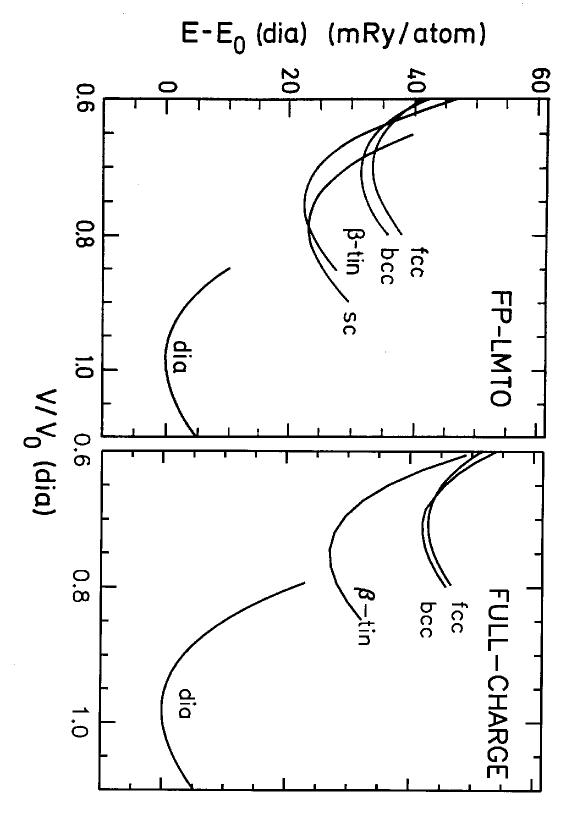
Figure 12: Total energy of Si as a function of the atomic volume for different structures calculated with the full-potential LMTO method [34] and with the present full-charge scheme [49, 47, 48]. See text.

Our fitting procedure [47] can be outlined as follows: We first place a set of screening spheres around each atomic site. This defines our screened Hankel functions (31) and divides space into non overlapping intra-sphere parts and an interstitial part. It is not necessary to place screening spheres at interstitial sites, even though the resulting interstitial can be very large. In the intra-sphere region we use a spherical-harmonics expansion of the charge density, with the components $\rho_{RL}(r)$ known on a radial mesh. As the screening spheres are relatively small this summation can be truncated at $l$=3 or 4. In the interstitial we expand in the screened Hankel functions, $n_{RL}^{a}\left(\varepsilon,\mathbf{r}_{R}\right),$ normalized as in (47) and with 3 different, negative energies, of which the lowest is about 4 times the work function, that is:

$$\rho(\mathbf{r}) \approx \sum_{n=0}^{2}\sum_{RL}n_{RL}^{a}\left(\varepsilon_{n},\mathbf{r}_{R}\right)\,\lambda_{RL;n}=\sum_{RL}\breve{n}_{RL}^{a}\left(\mathbf{r}_{R}\right)\mu_{RL}+$$

$$\quad\quad\sum_{RL}\left(n_{RL}^{a}\left(\mathbf{r}_{R}\right)\rho_{RL}\left(a\right)+n_{RL}^{a}\left(\left[01\right],\mathbf{r}_{R}\right)\sum_{R^{\prime}L^{\prime}}X_{RL,R^{\prime}L^{\prime}}\,\rho_{R^{\prime}L^{\prime}}\right)$$

for all $r_{R}\geq a_{RL}.$ With three energies, we can in principle fit continuously with continuous 1st and 2nd derivatives. However, in practice it is difficult to compute the 2nd radial derivatives of the high-$l$ components of the charge density. We therefore determine the matrix $X$ in such a way that the fitting is continuous and once differentiable, that is: $X=B^{a}\left[01\right]^{-1}\left(\partial\left\{\rho\left(a\right)\right\}-B_{0}^{a}\right).$ The functions $\breve{n}_{RL}^{a}\left(\mathbf{r}_{R}\right)$ in (3.2.7) are those linear combinations of the three $n^{a}\left(\varepsilon_{n},\mathbf{r}\right)$’s whose value and radial slope vanish in all channels at the screening spheres. These functions therefore peak in the interstitial region and their coefficients $\mu_{RL}$ are determined by a least squares fit in the region interstitial to the MT-spheres, by sampling the full charge (109), as well as the expansion (3.2.7) at a set of pseudo-random points. Once the expansion is obtained, it is very easy to solve Poisson’s equation. In the intra-sphere part this is done numerically and in the interstitial analytically by virtue of the screened Hankel functions solving the wave equation. The same expansion procedure can be applied to the exchange-correlation energy density $\epsilon(\mathbf{r})$ and potential $\mu(\mathbf{r})$. This gives a full potential. The total energy $E_{tot}$ is also easy to evaluate. The interstitial part of the integrals reduces simply to a summation over Hermite divided differences of the slope matrix.

We have applied this procedure to look at the total energy of various possible structures for silicon [49]. For each structure we perform a standard self consistent LMTO-ASA calculation. In the last iteration an expansion of the full charge density is made and $E_{tot}$ evaluated correctly. The result is shown in Fig. 12 where, for comparison, we show the full-potential LMTO result from Ref. [34].

Figure 13: Rms error of the valence-band energies in diamond-structured Si as a function of the overlap in the atom-centered MT-potential [42, 43]. See text.

3.2.8 Overlapping MT-potential: Si without empty spheres.

The phase diagram of Si just shown was calculated using LMTOs defined for MT-potentials with empty spheres. We now consider the possibility offered by Eq. (2.1) of allowing the atom-centered sphere a substantial overlap –like the 50% radial overlap shown in Figs. 2-5– and, hence, of getting rid of the empty spheres.

The first question is: How to construct such a potential? Our answer is [42] that the potential should be constructed such as to minimize the mean squared deviation of the valence-band energies from the ones for the full potential. From this condition, it then follows that the overlapping MT-potential, $\sum_{R}v\left(r_{R}\right),$ should be the least-squares approximation to the full-potential, $V\left(\mathbf{r}\right)$, weighted with the valence charge density. This yields a set of coupled equations for the shape, $f\left(r\right)\equiv v\left(r\right)-g,$ and the zero, $g,$ of the MT-potential. The equation which arises from requiring stationarity with respect to $\delta g$ is of course: $\int\left(V-\sum v\right)\rho d^{3}r=0,$ and it means that the error in the sum of the valence-band energies should vanish to leading order. The other equations, which arise by requiring stationarity with respect to $\delta f\left(r\right),$ are coupled integral equations, which are complicated due to the presence of the charge-density weighting. Taking the charge density to be constant in space, corresponds to minimizing the mean squared energy-deviation for the entire spectrum, rather than merely for the valence band. Now, in our present implementation, we only took the spatial behavior of the charge density into account in the $\delta g$-equation. The resulting potentials for diamond-structured Si were shown in Figs. 10 and 11 of Ref. [20]. We have recently succeeded in obtaining the overlapping MT potential from the full potential obtained from the charge density (3.2.7) [43], but in the present paper we shall only show results obtained by taking the full potential to be the Si+E ASA potential –like in Ref. [20].

Figure 14: Band structure of Si calculated with the 3rd-generation LMTO method for the self-consistent Si+E MT-potential (dashed) and for the Si-centered, 60%-overlapping MT-approximation to it (solid). The latter calculation included the correction for the kinetic-energy error Eq. (2.1) in the LMTO Hamiltonian, and the value of the MT-zero was adjusted in such a way that the average energy of the valence band was correct. Hence, the solid band structure corresponds to the last point on the curve marked ’ideal’ in Fig. 13 [42, 43]. See text.

Fig. 13 shows three different results for the rms error of the valence-band energy as a function of the linear overlap, $\omega\equiv\left(s/t\right)-1.$ For the overlap increasing up to about 30%, the rms error falls in all cases, simply because the overlapping MT-potential becomes an increasingly better approximation to the full potential. Without any overlap correction, the kinetic-energy error (2.1), which is of second order in the potential overlap, initially rises proportional to $v\left(s\right)^{2}\omega^{4}$ [20], and this is seen to limit the maximum overlap to about 30%. We may, however, use the LMTO equivalent [43] of Eq. (2.1) to correct each band energy, $\varepsilon_{i}\left(\mathbf{k}\right),$ and the results are shown by the two other curves. The dashed curve –marked ’present technique’– uses the $\delta g$-equation as given above, whereas the ’ideal’ curve was obtained by adjusting $g$ –iteratively, because $g$ enters the $\delta f\left(r\right)$ equations– to have the mean error of the valence-band energy vanish exactly. It is possible to improve upon the ’present technique’ without knowing the valence-band energy a priori, and we are currently including charge-density weighting in the $\delta f\left(r\right)$-equations. This makes the curve flatten out –like the one marked ’ideal’ [43].

The solid curves in Fig. 14 show the Si band structure obtained with the 60% overlapping MT-potential, including the LMTO overlap correction, and determining $g$ to yield vanishing mean error of the valence band. The dotted curve is the ’exact’ result as obtained with a (3rd-generation) LMTO calculation for the Si+E potential. The errors seen in the valence band are certainly no larger than 30 meV, but those in the conduction band are larger.

4 Energy-dependent linear transformations

If one considers Fig. 1, it might seem as if the energy-window over which an NMTO set yields good approximations to the wave functions will be wider if one starts out from energy-dependent linear combinations of kinked partial waves:

$$\hat{\phi}\left(\varepsilon,\mathbf{r}\right)\;\equiv\;\phi\left(\varepsilon,\mathbf{r}\right)\hat{T}\left(\varepsilon\right),$$ (111)

which have smoother energy dependencies. Normalized kinked partial waves and Löwdin orthonormalized kinked partial waves are examples of cases where the divergences of the kinked partial waves at the energies, $\varepsilon_{RL}^{a},$ where a node passes through the screening radius, are avoided. The transformation given by the – in general non-Hermitian – matrix $\hat{T}\left(\varepsilon\right)$ mixes kinked partial waves with the same energy and different $RL$’s linearly. Although the Hilbert spaces spanned by the energy-dependent sets, $\phi\left(\varepsilon,\mathbf{r}\right)$ and $\hat{\phi}\left(\varepsilon,\mathbf{r}\right),$ are identical, it is not obvious that those spanned by the respective polynomial approximations, $\chi^{\left(N\right)}\left(\mathbf{r}\right)$ and $\hat{\chi}^{\left(N\right)}\left(\mathbf{r}\right),$ are also identical, particularly not if one bears only Fig. 1 in mind.

Depending on the transformation, the resulting $\hat{\phi}\left(\varepsilon,\mathbf{r}\right)$ may completely have lost its original $RL$-character. Since the linear combination, $\hat{\phi}\left(\varepsilon,\mathbf{r}\right),$ of kinked partial waves has active radial functions on other sites, as well as at its own site for other $L$’s, it is not a kinked partial wave in the usual sense, that is, one which could have been obtained by a screening transformation. Remember, that for 3rd-generation kinked partial waves, a screening transformation is not linear. In the following, we shall assume that the screening radii have been chosen at the previous step, in the screening calculation for the structure matrix, and perhaps by subsequent re-screening of the $G_{n}$’s using (57).

A further motivation for considering transformed kinked partial waves is that they might provide the freedom to obtain energy matrices (83) which are Hermitian. This would simplify the finite-difference expressions (3.1.4) and (3.1.4) for the NMTO so that they take the simpler form (1) which then –like in (3)– could be diagonalized to leading order by the eigenvectors of $\hat{E}^{\left(N\right)}.$ From expression (87) for the transfer matrix, we realize that the condition that a transformed $\hat{E}^{\left(M\right)}$ be a Hamiltonian matrix, is that we can find a transformation with the property that

$$\left\langle\hat{\chi}^{\left(M\right)}\mid\hat{\chi}^{\left(M-1\right)}\right\rangle\;=\;1.$$ (112)

This formalism could therefore also be the basis for obtaining an orthonormal NMTO set.

Let us finally express the important equations (59)-(2.5) in terms of the transformed kinked partial waves:

$$\left(\mathcal{H}-\varepsilon\right)\hat{\phi}\left(\varepsilon,\mathbf{r}\right)=-\delta\left(\mathbf{r}\right)\hat{K}\left(\varepsilon\right),\mathrm{\;}\left(\mathcal{H}-\varepsilon\right)\hat{\phi}\left(\varepsilon,\mathbf{r}\right)\hat{G}\left(\varepsilon\right)=-\delta\left(\mathbf{r}\right),$$ (113)

where we have defined the non-Hermitian matrices

$$\hat{K}\left(\varepsilon\right)\equiv K\left(\varepsilon\right)\hat{T}\left(\varepsilon\right),\mathrm{\quad\quad}\hat{G}\left(\varepsilon\right)\equiv\hat{K}\left(\varepsilon\right)^{-1}=\hat{T}\left(\varepsilon\right)^{-1}G\left(\varepsilon\right).$$ (114)

Note that these definitions do not correspond to similarity transformations. The kink matrix, $K\left(\varepsilon\right),$ and thereby its inverse, $G\left(\varepsilon\right),$ were originally defined in such a way that they are Hermitian, but they are inherently ’skew’, because (113) tells us that it is the ’one-sided’ contraction of the Green function,

$$\gamma\left(\varepsilon,\mathbf{r}\right)=\phi\left(\varepsilon,\mathbf{r}\right)G\left(\varepsilon\right)=\hat{\phi}\left(\varepsilon,\mathbf{r}\right)\hat{G}\left(\varepsilon\right),$$ (115)

which is invariant. For the same reason, the integrals of the products of two contracted Green functions, with possibly different energies, form an overlap matrix,

$$\hat{G}\left(\varepsilon\right)^{\dagger}\left\langle\hat{\phi}\left(\varepsilon\right)\mid\hat{\phi}\left(\varepsilon^{\prime}\right)\right\rangle\hat{G}\left(\varepsilon^{\prime}\right)=-\frac{G\left(\varepsilon\right)-G\left(\varepsilon^{\prime}\right)}{\varepsilon-\varepsilon^{\prime}},$$ (116)

which is independent of $\hat{T}\left(\varepsilon\right).$

Adding to the discussion following (94) about the meaning of the matrix equation $\left\langle\phi_{n}\mid\phi_{n^{\prime}}\right\rangle=\left\langle\phi_{n^{\prime}}\mid\phi_{n}\right\rangle,$ note that this equation does not hold in a general representation: $\left\langle\hat{\phi}_{n}\mid\hat{\phi}_{n^{\prime}}\right\rangle=\hat{T}_{n}^{\dagger}\hat{T}_{n^{\prime}}^{\dagger-1}\left\langle\hat{\phi}_{n^{\prime}}\mid\hat{\phi}_{n}\right\rangle\hat{T}_{n}^{-1}\hat{T}_{n^{\prime}}\neq\left\langle\hat{\phi}_{n^{\prime}}\mid\hat{\phi}_{n}\right\rangle,$ unless$\;\hat{T}_{n}=\hat{T}_{n^{\prime}}.$ But it is of course always true that$\;\left\langle\hat{\phi}_{n}\mid\hat{\phi}_{n^{\prime}}\right\rangle=\left\langle\hat{\phi}_{n^{\prime}}\mid\hat{\phi}_{n}\right\rangle^{\dagger}.$

We now come to derive NMTOs from the transformed kinked partial waves (111). Since the arguments around expression (71) concerned the contracted Green function, which according to (115) is invariant, (71) is unchanged but should be rewritten in the form:

$$\hat{\chi}^{\left(N\right)}\left(\varepsilon,\mathbf{r}\right)\hat{G}\left(\varepsilon\right)=\hat{\phi}\left(\varepsilon,\mathbf{r}\right)\hat{G}\left(\varepsilon\right)-\sum_{n=0}^{N}\hat{\phi}_{n}\left(\mathbf{r}\right)\,\hat{G}_{n}\,A_{n}^{\left(N\right)}\left(\varepsilon\right).$$ (117)

As a consequence, (72) should be substituted by:

$$\hat{\chi}^{\left(N\right)}\left(\mathbf{r}\right)=\frac{\Delta^{N}\hat{\phi}\left(\mathbf{r}\right)\hat{G}}{\Delta\left[0..N\right]}\left(\frac{\Delta^{N}\hat{G}}{\Delta\left[0..N\right]}\right)^{-1}=\frac{\Delta^{N}\phi\left(\mathbf{r}\right)G}{\Delta\left[0..N\right]}\left(\frac{\Delta^{N}\hat{G}}{\Delta\left[0..N\right]}\right)^{-1}.$$ (118)

The last equation (118) shows that the polynomial approximation to the transformed energy-dependent NMTO, $\hat{\chi}^{\left(N\right)}\left(\varepsilon,\mathbf{r}\right)=\chi^{\left(N\right)}\left(\varepsilon,\mathbf{r}\right)\hat{T}\left(\varepsilon\right),$ is

$$\hat{\chi}^{\left(N\right)}\left(\mathbf{r}\right)=\chi^{\left(N\right)}\left(\mathbf{r}\right)\,G\left[0...N\right]\,\hat{G}\left[0...N\right]^{-1},$$ (119)

which is a linear transformation. Hence, regardless of the energy-dependent transformation $\hat{T}\left(\varepsilon\right)$ of the kinked partial waves, all NMTO sets span the same Hilbert space and all energy-windows are therefore identical. This disproves the above-mentioned naive conclusion drawn from Fig. 1. Since $G\left(\varepsilon\right)=\hat{T}\left(\varepsilon\right)\hat{G}\left(\varepsilon\right),$ we may express the NMTO transformation (119) as a Newton series (3.1.4) for $\hat{T}\left(\varepsilon\right):$

$$G\left[0...N\right]\,\hat{G}\left[0...N\right]^{-1} = \left(\hat{T}\hat{G}\right)\left[0...N\right]\,\hat{G}\left[0...N\right]^{-1}$$

$$= \sum\nolimits_{M=0}^{N}\hat{T}\left[0..M\right]\,\hat{G}\left[M..N\right]\,\hat{G}\left[0...N\right]^{-1}$$

$$= \hat{T}_{0}+..+\hat{T}\left[0...N\right]\left(\hat{E}^{\left(1\right)}-\varepsilon_{N-1}\right)..\left(\hat{E}^{\left(N\right)}-\varepsilon_{0}\right).$$

Since the contracted Green function is invariant, so are equations (94) and (95) which relate the overlap and Hamiltonian integrals of such functions to Hermite divided differences of $G\left(\varepsilon\right).$ For the NMTO overlap and Hamiltonian matrices, we therefore obtain (96) and (97), with the prefactor substituted by $\hat{G}\left[0..N\right]^{-1\dagger},$ the postfactor substituted by $\hat{G}\left[0..N\right]^{-1},$ and the Hermite divided differences of $G\left(\varepsilon\right)$ unaltered.

The first equation (118) shows that the expressions derived previously for the NMTOs, excluding those for integrals over NMTOs, may be taken over, after these expressions have been subject to the following substitutions:

$$\begin{array}[]{ccccc}\phi\left(\varepsilon,\mathbf{r}\right)\rightarrow\hat{\phi}\left(\varepsilon,\mathbf{r}\right),&&K\left(\varepsilon\right)\rightarrow\hat{K}\left(\varepsilon\right),&&L_{n}^{\left(N\right)}\rightarrow\hat{L}_{n}^{\left(N\right)},\\ \chi\left(\varepsilon,\mathbf{r}\right)\rightarrow\hat{\chi}\left(\varepsilon,\mathbf{r}\right),&&G\left(\varepsilon\right)\rightarrow\hat{G}\left(\varepsilon\right),&&E^{\left(M\right)}\rightarrow\hat{E}^{\left(M\right)}.\end{array}$$ (121)

Remember, that the substitutions for $K\left(\varepsilon\right)$ and $G\left(\varepsilon\right)$ do not correspond to a similarity transformation.

As long as we only consider $\hat{T}\left(\varepsilon\right)$-transformations which are independent of $N$, the step-down relation (82) holds for the transformed NMTOs and for its transfer matrices, because the derivation merely made use of (59), which transforms into (113). This shows that $\hat{E}^{\left(0\right)}-\varepsilon_{0}$ equals $-\hat{K}_{0}=-K_{0}\hat{T}_{0},$ as expected, but that: $\left\langle\hat{\chi}^{\left(0\right)}\mid\hat{\chi}^{\left(-1\right)}\right\rangle=1$ does not hold. The hatted version of (87) therefore only holds for $N\geq 1.$ For $N=0:$

$$\left\langle\hat{\chi}^{\left(0\right)}\left|\mathcal{H}-\varepsilon_{0}\right|\hat{\chi}^{\left(0\right)}\right\rangle=-\hat{T}_{0}^{\dagger}K_{0}\hat{T}_{0}=\hat{T}_{0}^{\dagger}\left(\hat{E}^{\left(0\right)}-\varepsilon_{0}\right)\equiv\hat{H}^{\left(0\right)}-\varepsilon_{0}.$$ (122)

The expressions for the transformed NMTO in terms of divided differences of transformed kinked partial waves are the hatted versions of (3.1.4) and (3.1.4). One should remember that the divided difference, $\hat{\phi}\left(\left[0..M\right],\mathbf{r}\right),$ is a linear combination of the $M+1$ functions $\phi_{0}\left(\mathbf{r}\right)\hat{T}_{0},..,\phi_{M}\left(\mathbf{r}\right)\hat{T}_{M},$ and hence, a linear combination of the $M+1$ divided differences: $\phi_{0}\left(\mathbf{r}\right),\,..,\phi\left(\left[0..M\right],\mathbf{r}\right)$. This is the generalization of the property: $d\phi\left(\varepsilon,\mathbf{r}\right)\hat{T}\left(\varepsilon\right)\left/d\varepsilon\right|_{\varepsilon_{\nu}}=\dot{\phi}\left(\mathbf{r}\right)\hat{T}+\phi\left(\mathbf{r}\right)\overset{.}{\hat{T}},$ used in the 2nd-generation LMTO formalism. Explicitly:

$$\hat{\phi}\left(\left[0...M\right],\mathbf{r}\right)=\sum_{n=0}^{M}\frac{\phi_{n}\left(\mathbf{r}\right)\hat{T}_{n}}{\prod_{m=0,\neq n}^{M}\left(\varepsilon_{n}-\varepsilon_{m}\right)}$$

$$= \sum_{m=0}^{M}\phi\left(\left[m..M\right],\mathbf{r}\right)\hat{T}\left[0..m\right]=\phi\left(\left[0...M\right],\mathbf{r}\right)\hat{T}_{0}+..+\phi_{M}\left(\mathbf{r}\right)\hat{T}\left[0...M\right].$$

The transformed versions of the results (3.2.6), (3.2.6) are complicated, unless $\hat{T}\left(\varepsilon\right)$ is independent of $\varepsilon.$ In that case, the right-hand sides just have $K\left(\varepsilon\right)$ substituted by $\hat{T}^{\dagger}K\left(\varepsilon\right)\hat{T}\equiv\bar{K}\left(\varepsilon\right).$

Usually $\left\langle\hat{\phi}\left[0..M\right]\mid\hat{\phi}\left[0..N\right]\right\rangle\neq\left\langle\hat{\phi}\left[0..N\right]\mid\hat{\phi}\left[0..M\right]\right\rangle,$ unless $\hat{T}\left(\varepsilon\right)=\hat{T},$ or the matrix is diagonal; $\left\langle\hat{\phi}\left[0..M\right]\mid\hat{\phi}\left[0..N\right]\right\rangle=\left\langle\hat{\phi}\left[0..N\right]\mid\hat{\phi}\left[0..M\right]\right\rangle^{\dagger}$ of course always holds.

5 Hamiltonian energy matrices and orthonormal sets

Having seen that an energy-dependent, linear transformation (111) of the MTO set does not change the Hilbert space spanned by the set of energy-independent NMTOs, but merely the individual basis functions, we now turn to the objective of finding a representation in which the energy matrices $\hat{E}^{\left(M\right)}$ –but not necessarily the Green matrix $\hat{G}\left(\varepsilon\right)$– are Hermitian. The energy matrices will then be the two-center Hamiltonians entering expressions like (1) for the orbitals. From (87), we obviously want:

$$\hat{E}^{\left(M\right)}-\varepsilon_{M}=\left\langle\hat{\chi}^{\left(M\right)}\left|\mathcal{H}-\varepsilon_{M}\right|\hat{\chi}^{\left(M\right)}\right\rangle\equiv\hat{H}^{\left(M\right)}-\varepsilon_{M}$$ (124)

for$\;1\leq M\leq N,$ and since this condition leads to the near-orthonormality condition (112), it guides the way to make one of the NMTO sets –let us call it the $L$th– orthonormal.

In order to solve the $N$ near-orthonormality conditions for the Hamiltonian matrices, we first insert the transformed version of expression (85) for the inverse of the $M$th divided difference of the Green matrix in terms of the transfer matrices and $\hat{H}^{\left(0\right)}-\varepsilon_{0},$ defined by (122),

$$-\hat{G}\left[0...M\right]^{-1}=\hat{T}_{0}^{-1\dagger}\left(\hat{H}^{\left(0\right)}-\varepsilon_{0}\right)\left(\hat{H}^{\left(1\right)}-\varepsilon_{1}\right)..\left(\hat{H}^{\left(M\right)}-\varepsilon_{M}\right),$$ (125)

into the transformed version of expression (97) for the Hamiltonian in terms of the $2M$th Hermite divided difference of the original Green matrix $G\left(\varepsilon\right).$ We then use (124) and notice that one factor $\hat{H}^{\left(M\right)}-\varepsilon_{M}$ cancels out so that the equation may be solved for this highest transfer matrix:

$$\hat{H}^{\left(M\right)}-\varepsilon_{M}=\left[\begin{array}[]{l}\left(\hat{H}^{\left(M-1\right)}-\varepsilon_{M-1}\right)..\left(\hat{H}^{\left(1\right)}-\varepsilon_{1}\right)\left(\hat{H}^{\left(0\right)}-\varepsilon_{0}\right)\\ \quad\times\hat{T}_{0}^{-1}\left(-G\left[\left[0..M-1\right]M\right]\right)\hat{T}_{0}^{-1\dagger}\\ \quad\quad\times\left(\hat{H}^{\left(0\right)}-\varepsilon_{0}\right)\left(\hat{H}^{\left(1\right)}-\varepsilon_{1}\right)..\left(\hat{H}^{\left(M-1\right)}-\varepsilon_{M-1}\right)\end{array}\right]^{-1}$$

for $M\geq 1$. Solving recursively for the transfer matrices, and including (122) at the top, we obtain the following results:

$$\hat{H}^{\left(0\right)}-\varepsilon_{0} = -\hat{T}_{0}^{\dagger}G\left[\left[\;\right]0\right]^{-1}\hat{T}_{0}$$

$$\hat{H}^{\left(1\right)}-\varepsilon_{1} = -\hat{T}_{0}^{-1}G\left[\left[\;\right]0\right]\,G\left[\left[0\right]1\right]^{-1}G\left[\left[\;\right]0\right]\hat{T}_{0}^{-1\dagger}$$

$$\hat{H}^{\left(2\right)}-\varepsilon_{2} = -\hat{T}_{0}^{\dagger}G\left[\left[\;\right]0\right]^{-1}G\left[\left[0\right]1\right]\,G\left[\left[01\right]2\right]^{-1}G\left[\left[0\right]1\right]\,G\left[\left[\;\right]0\right]^{-1}\hat{T}_{0}$$

$$\hat{H}^{\left(M\right)}-\varepsilon_{M} = -\hat{T}_{0}^{\left(-1\right)^{M}\left(\dagger\right)^{M+1}}G\left[\left[\;\right]0\right]^{\left(-1\right)^{M+1}}...\,G\left[\left[0..M-1\right]M\right]^{-1}$$ (126)

$$\quad\quad\quad\quad\quad\quad\quad...G\left[\left[\;\right]0\right]^{\left(-1\right)^{M+1}}\hat{T}_{0}^{\left(-1\right)^{M}\left(\dagger\right)^{M}},$$

where for reasons of systematics we have used the notation (162):

$$G\left[\left[\;\right]0\right]=G\left[0\right]=G_{0}=K_{0}^{-1},$$

explained in the Appendix.

The divided differences (125) of the transformed Green matrix are needed for specification of the transformation via (114), the orbitals via (119), or the transformed kinked partial waves via (115), and are seen to be given by:

$$\hat{G}\left[0\right]^{-1} = \;G\left[\left[\;\right]0\right]^{-1}\hat{T}_{0}$$

$$\hat{G}\left[01\right]^{-1} = -G\left[\left[0\right]1\right]^{-1}G\left[\left[\;\right]0\right]\hat{T}_{0}^{-1\dagger}$$ (127)

$$\hat{G}\left[012\right]^{-1} = \;G\left[\left[01\right]2\right]^{-1}G\left[\left[0\right]1\right]\,G\left[\left[\;\right]0\right]^{-1}\hat{T}_{0}$$

$$\hat{G}\left[0...M\right]^{-1} = \left(-\right)^{M}G\left[\left[0..M-1\right]M\right]^{-1}...G\left[\left[\;\right]0\right]^{\left(-1\right)^{M+1}}\hat{T}_{0}^{\left(-1\right)^{M}\left(\dagger\right)^{M}}.$$

Since we originally had the $N+1$ matrices $\hat{T}_{0}...\hat{T}_{N}$ at our disposal and have used $N$ to satisfy the near-orthonormality conditions, we have one, $\hat{T}_{0},$ left. This –and thereby implicitly also the other $\hat{T}_{n}$’s– may now be chosen equal to a matrix, $\check{T}_{0},$ which makes the $L$th set orthonormal. Note that whereas the transformation $\hat{T}\left(\varepsilon\right)$ did not depend on the order of any basis set, the transformation $\check{T}\left(\varepsilon\right)$ does; it depends on $L$.

Let us first discuss whether the transformation (100) to an orthonormalized NMTO set may at all be arrived at by an energy-dependent linear transformation of the kinked partial waves: According to (119), othonormality of the $L$th set happens for any transformation $\check{T}\left(\varepsilon\right)$ which satisfies: $\left(\check{T}^{-1}G\right)\left[0...L\right]=\left(-G\left[\left[0...L\right]\right]\right)^{1/2},$ where $G\left[\left[0..L\right]\right]$ is the $(2L+1)$st Hermite divided difference (160) of the original Green matrix. Hence, this is a linear equation between the $L+1$ values of the matrix $\check{T}\left(\varepsilon\right)^{-1}$ at the first $L+1$ mesh points, and it is therefore plausible that it may be used to fix $\check{T}_{0}.$

The better way of writing this equation is, like for the Hamiltonian matrix, to insert (125) for $\hat{G}\left[0..L\right]^{-1}$ into the transformed version of expression (96) for the overlap matrix. As a result:

$$\left\langle\hat{\chi}^{\left(L\right)}\mid\hat{\chi}^{\left(L\right)}\right\rangle=\left(\hat{H}^{\left(L\right)}-\varepsilon_{L}\right)..\left(\hat{H}^{\left(1\right)}-\varepsilon_{1}\right)\left(\hat{H}^{\left(0\right)}-\varepsilon_{0}\right)\times$$

$$\hat{T}_{0}^{-1}\left(-G\left[\left[0..L\right]\right]\right)\hat{T}_{0}^{-1\dagger}\left(\hat{H}^{\left(0\right)}-\varepsilon_{0}\right)\left(\hat{H}^{\left(1\right)}-\varepsilon_{1}\right)..\left(\hat{H}^{\left(L\right)}-\varepsilon_{L}\right)$$

$$= -\hat{T}_{0}^{\left(-1\right)^{L}\left(\dagger\right)^{L+1}}G\left[\left[\;\right]0\right]^{\left(-1\right)^{L+1}}..G\left[\left[0..L\right]\right]..G\left[\left[\;\right]0\right]^{\left(-1\right)^{L+1}}\hat{T}_{0}^{\left(-1\right)^{L}\left(\dagger\right)^{L}}.$$

We see that the equation $\left\langle\hat{\chi}^{\left(L\right)}\mid\hat{\chi}^{\left(L\right)}\right\rangle=1$, in contrast to the equation: $\left\langle\hat{\chi}^{\left(M\right)}\left|\mathcal{H}-\varepsilon_{M}\right|\hat{\chi}^{\left(M\right)}\right\rangle=\hat{H}^{\left(M\right)}-\varepsilon_{M}$, is quadratic in all Hamiltonians, and therefore can only be solved by taking the square root of a matrix.

Hence, our strategy is to choose a $\hat{T}_{0},$ which makes the non-orthonormality,

$$\left\langle\hat{\chi}^{\left(L\right)}\mid\hat{\chi}^{\left(L\right)}\right\rangle-1\;\equiv\;\hat{O}^{\left(L\right)},$$ (129)

so small, that we may use an expansion like (102) to find $\check{T}_{0}$ and the corresponding Hamiltonians $\check{H}^{\left(M\right)}.$ Of these, $\check{H}^{\left(L\right)}$ equals the variational Hamiltonian (3.2.2) with $N$ substituted by $L,$ and its eigenvalues are therefore correct to order $2L+1.$ Expression (5) now tells us that:

$$\hat{T}_{0}^{\left(-1\right)^{L+1}\left(\dagger\right)^{L+1}}\left\langle\hat{\chi}^{\left(L\right)}\mid\hat{\chi}^{\left(L\right)}\right\rangle\hat{T}_{0}^{\left(-1\right)^{L+1}\left(\dagger\right)^{L}}=\check{T}_{0}^{\left(-1\right)^{L+1}\left(\dagger\right)^{L+1}}\check{T}_{0}^{\left(-1\right)^{L+1}\left(\dagger\right)^{L}},$$

which may be solved to yield:

$$\check{T}_{0}=\hat{T}_{0}\sqrt{1+\hat{O}^{\left(L\right)}}^{\left(-1\right)^{L+1}}=\hat{T}_{0}\left\{\begin{array}[]{l}1+\frac{1}{2}\hat{O}^{\left(L\right)}-\frac{1}{8}\left(\hat{O}^{\left(L\right)}\right)^{2}+..\\ 1-\frac{1}{2}\hat{O}^{\left(L\right)}+\frac{3}{8}\left(\hat{O}^{\left(L\right)}\right)^{2}-..\end{array}\right.$$ (130)

Here, the upper result is for $L$ odd and the lower for $L$ even. Since $\hat{O}^{\left(L\right)}$ will be chosen small, and for $L>1$ is usually of order $\left(\varepsilon_{i}-\varepsilon_{1}\right)\left(\varepsilon_{i}-\varepsilon_{0}\right),$ as we shall argue in (145) and (152), this transformation preserves the $RL$-character of each NMTO. The Hamiltonian matrix (126) is seen to transform like the overlap matrix (5) with $M$ substituted for $L$ and, as a consequence,

$$\check{H}^{\left(M\right)}-\varepsilon_{M}=$$

$$\sqrt{1+\hat{O}^{\left(L\right)}}^{\left(-1\right)^{L-M+1}}\left(\hat{H}^{\left(M\right)}-\varepsilon_{M}\right)\sqrt{1+\hat{O}^{\left(L\right)}}^{\left(-1\right)^{L-M+1}}.$$ (131)

Similarly, from (127):

$$\check{G}\left[0...M\right]^{-1}\;=\;\hat{G}\left[0...M\right]^{-1}\sqrt{1+\hat{O}^{\left(L\right)}}^{\left(-1\right)^{L-M+1}}.$$ (132)

A procedure for computing $\left[1+O\right]^{\pm\frac{1}{2}},$ which is more robust than the matrix Taylor series (130), is included in our codes [60].

5.0.1 Choosing $\hat{T}_{0}.$

Since the near-orthonormality conditions (112) merely fix the geometrical average $\left\langle\hat{\chi}^{\left(M\right)}\mid\hat{\chi}^{\left(M-1\right)}\right\rangle$ of successive sets, the nearly orthonormal scheme (126)-(5) only makes sense if the transformation $\hat{T}_{0}$ of the kinked partial waves at $\varepsilon_{0}$ is chosen in such a way that the non-orthonormality $\hat{O}^{\left(0\right)}$ is small compared with the unit matrix. The nearly-orthonormal scheme alone, does not make the orthonormalization integrals $\left\langle\hat{\chi}^{\left(M\right)}\mid\hat{\chi}^{\left(M\right)}\right\rangle$ converge towards the unit matrix, but make them behave like:

$$\left\langle\hat{\chi}^{\left(M\right)}\mid\hat{\chi}^{\left(M\right)}\right\rangle\;\sim\;\left\langle\hat{\chi}^{\left(0\right)}\mid\hat{\chi}^{\left(0\right)}\right\rangle^{\left(-1\right)^{M}}.$$

This alternates with fluctuations depending on the size of $\left\langle\hat{\chi}^{\left(0\right)}\mid\hat{\chi}^{\left(0\right)}\right\rangle.$

The first thing to do is therefore to renormalize the MTOs in such a way that $\hat{T}_{0}^{a\dagger}\left\langle\left|\phi_{RL}^{a}\right|^{2}\right\rangle\hat{T}_{0}^{a}=1,$ instead of (49). Hence, the first choice is:

$$\hat{T}_{0}^{a}\;=\;\left(\dot{k}_{0}^{a}\right)^{-\frac{1}{2}}$$ (133)

where $\dot{k}_{0}^{a}$ is the energy-independent diagonal matrix with elements

$$\left\langle\left|\phi_{RL}^{a}\left(\varepsilon_{0}\right)\right|^{2}\right\rangle\;=\;\dot{K}_{RL,RL}^{a}\left(\varepsilon_{0}\right)\;\equiv\;\dot{k}_{RL,RL}^{a}\left(\varepsilon_{0}\right).$$ (134)

Another choice is to start with a Löwdin orthonormalized 0th-order set:

$$\hat{T}_{0}^{a}\;=\;\left(\dot{k}_{0}^{a}\right)^{-\frac{1}{2}}\sqrt{1+O^{a}}^{-1}$$ (135)

where $O^{a}$ is the non-orthonormality of the 0th-order, renormalized MTO set:

$$O^{a}\;\equiv\;\left(\dot{k}_{0}^{a}\right)^{-\frac{1}{2}}\dot{K}_{0}^{a}\left(\dot{k}_{0}^{a}\right)^{-\frac{1}{2}}-1.$$ (136)

This choice therefore corresponds to taking $L=0.$

5.0.2 Test case: GaAs.

We have tested this orthonormalization method for GaAs using the minimal Ga $spd$ As $sp$ basis set and going all the way up to $L=3,$ that is, to a CMTO basis with the properties that $\check{H}^{\left(3\right)}=\left\langle\check{\chi}^{\left(3\right)}\left|\mathcal{H}\right|\check{\chi}^{\left(3\right)}\right\rangle$ and $\left\langle\check{\chi}^{\left(3\right)}\mid\check{\chi}^{\left(3\right)}\right\rangle=1,$ so that $\check{H}^{\left(3\right)}$ is a 7th-order Hamiltonian. $\check{H}^{\left(2\right)}$ and $\check{H}^{\left(1\right)}$ are of lower order, however, and neither of the three Hamiltonians commute.

We diagonalized $\check{H}^{\left(L\right)}$ for $L=1,2,3$ and compared with the band structures obtained with the corresponding non-orthonormal variational method discussed in Sect. 3.2. Both starting choices (133) and (135) were tried, and both gave fast convergence of the square-root expansions. The first choice which only requires evaluation of a square root at the last stage (131) but whose non-orthonormality $\hat{O}^{\left(L\right)}$ is larger, was found to be the fastest [24].

5.0.3 Aleph-representation.

The renormalization (133) is of the same nature as –but simpler than (due to lack of energy dependence)– the one performed in Subsection 2.3, where we went from phase-shift normalization to screening-sphere normalization. That diagonal transformation was given by (47) for the screened spherical waves, by (48) and (49) for the 0th-order MTOs, and by (51) for the KKR matrix. Since we distinguished between those two normalizations by using respectively Greek and Latin superscripts for the screening, e.g. $\alpha$ and $a,$ and since it is irrelevant, whether one arrives at a nearly orthonormal representation from quantities normalized one-or-another way, it is logical to label quantities having the integral normalization (133) by Hebraic superscripts, e.g. $\aleph$ as corresponding to the same screening as $\alpha$ and $a.$ Although not diagonal, and therefore influencing the shape of the kinked partial waves, also the Löwdin orthonormalization (135) is an energy-independent similarity transformation, and so is any of the following transformations:

$$\begin{array}[]{lll}\phi^{\aleph}\left(\varepsilon,\mathbf{r}\right)\;\equiv\;\phi^{a}\left(\varepsilon,\mathbf{r}\right)\hat{T}_{0}^{a}&&\chi^{\aleph\left(N\right)}\left(\varepsilon,\mathbf{r}\right)\;\equiv\;\chi^{a\left(N\right)}\left(\varepsilon,\mathbf{r}\right)\hat{T}_{0}^{a}\\ &&\\ K^{\aleph}\left(\varepsilon\right)\;\equiv\;\hat{T}_{0}^{a\,\dagger}\,K^{a}\left(\varepsilon\right)\,\hat{T}_{0}^{a}&&G^{\aleph}\left(\varepsilon\right)\;\equiv\;\hat{T}_{0}^{a\,-1}\,G^{a}\left(\varepsilon\right)\,\hat{T}_{0}^{a\,-1\,\dagger}\end{array}$$ (137)

with $\hat{T}_{0}^{a}$ arbitrary. From the latter energy-independent similarity transformation of $G\left(\varepsilon\right),$ the non-Hermitian matrices $L_{n}^{\left(N\right)}$ and $E^{\left(N\right)},$ which are given in terms of $G\left(\varepsilon\right)$ by respectively (75) and (83), are seen to transform like:

$$\begin{array}[]{ccc}L_{n}^{\aleph\left(N\right)}\;=\;\hat{T}_{0}^{a\,-1}L_{n}^{a\left(N\right)}\,\hat{T}_{0}^{a}&\quad\mathrm{and\quad}&E^{\aleph\left(M\right)}\;=\;\hat{T}_{0}^{a\,-1}E^{a\left(M\right)}\,\hat{T}_{0}^{a}\end{array}.$$ (138)

This –(137)-(138)– has all concerned an energy-independent similarity transformation of un-hatted quantities.

In order to ensure that the hatted quantities are independent of which representation –$a$ or $\aleph$– we start out from, e.g.

$$\hat{\phi}^{\aleph}\left(\varepsilon,\mathbf{r}\right)=\hat{\phi}^{a}\left(\varepsilon,\mathbf{r}\right)=\phi^{a}\left(\varepsilon,\mathbf{r}\right)\hat{T}^{a}\left(\varepsilon\right)=\phi^{\aleph}\left(\varepsilon,\mathbf{r}\right)\hat{T}^{\aleph}\left(\varepsilon\right)$$

and

$$\hat{G}^{\aleph}\left(\varepsilon\right)=\hat{G}^{a}\left(\varepsilon\right)=\hat{T}^{a}\left(\varepsilon\right)^{-1}G^{a}\left(\varepsilon\right)\hat{T}^{a}\left(\varepsilon\right)^{-1\dagger}=\hat{T}^{\aleph}\left(\varepsilon\right)^{-1}G^{\aleph}\left(\varepsilon\right)\hat{T}^{\aleph}\left(\varepsilon\right)^{-1\,\dagger}$$

where, from the latter, it follows that

$$\begin{array}[]{ccc}\hat{L}_{n}^{\aleph\left(N\right)}\;=\;\hat{L}_{n}^{a\left(N\right)}&\quad\mathrm{and\quad}&\hat{E}_{n}^{\aleph\left(M\right)}\;=\;\hat{E}_{n}^{a\left(M\right)}\end{array},$$

it suffices to satisfy the relation:

$$\begin{array}[]{ccccc}\hat{T}^{\aleph}\left(\varepsilon\right)\;\equiv\;\hat{T}_{0}^{a\,-1}\hat{T}^{a}\left(\varepsilon\right)\,,&&\mathrm{which\;leads\;to:}&&\hat{T}_{0}^{\aleph}=1.\end{array}$$ (139)

In conclusion, under the substitution $a\rightarrow\aleph,$ all previous equations remain valid, and the factors $\hat{T}_{0}^{\aleph}$ may be deleted.

The virtue of this notation is that, once we have decided upon the normalization and the screening, we can drop the superscripts; and this is what we shall do: From now on, and throughout the remainder of this paper, un-hatted quantities, i.e. the kinked partial waves, the kink and the Green matrices, and the Lagrange and energy matrices, are all supposed to have the integral (ortho)normalization (133) or (135), that is, they are all in the Aleph-representation. All equations derived previously are then unchanged, and $\hat{T}_{0}$ may be dropped.

5.0.4 Accuracies of Hamiltonians.

The accuracies of the Hamiltonians depend on the sizes of the corresponding non-orthonormalities. Specifically, since the residual error of the one-electron energy after use of the variational principle (5) for the set $\hat{\chi}^{\left(M\right)}\left(\mathbf{r}\right)$,

$$\hat{H}^{\left(M\right)}v_{i}=\,\varepsilon_{i}v_{i}+\left(\varepsilon_{i}-\varepsilon_{M}\right)\hat{O}^{\left(M\right)}v_{i}\,,$$

is proportional to $\left(\varepsilon_{i}-\varepsilon_{0}\right)^{2}..\left(\varepsilon_{i}-\varepsilon_{M}\right)^{2},$ neglect of the non-orthonormality, leads to the error:

$$\delta\hat{\varepsilon}_{i}^{\,\left(M\right)}\;=\;\left(\varepsilon_{i}-\varepsilon_{M}\right)\hat{O}_{ii}^{\left(M\right)}\;+\;\mathcal{O}\left\{\left(\varepsilon_{i}-\varepsilon_{0}\right)^{2}..\left(\varepsilon_{i}-\varepsilon_{M}\right)^{2}\right\},$$ (140)

where $\hat{O}_{ii}^{\left(M\right)}\equiv$ $v_{i}^{\dagger}\hat{O}^{\left(M\right)}v_{i}$ and $\mathcal{O}$ means at the order of. The goal should thus be to reduce the non-orthonormality to:

$$\hat{O}_{ii}^{\left(M\right)}\;=\;\mathcal{O}\left\{\left(\varepsilon_{i}-\varepsilon_{0}\right)^{2}..\left(\varepsilon_{i}-\varepsilon_{M-1}\right)^{2}\left(\varepsilon_{i}-\varepsilon_{M}\right)\right\}$$

because in that case, the error from non-orthonormality will be of the same order as that of the residual error. This can usually only achieved for $M=L.$

The order of the non-orthonormality may be found by use of the difference function:

$$\hat{\chi}^{\left(M\right)}\left(\mathbf{r}\right)-\hat{\chi}^{\left(M-1\right)}\left(\mathbf{r}\right)\;=\;\hat{\phi}\left(\left[01\right],\mathbf{r}\right)\left(\hat{H}^{\left(M\right)}-\hat{H}^{\left(M-1\right)}\right)+\;\hat{\phi}\left(\left[012\right],\mathbf{r}\right)$$

$$\quad\quad\quad\quad\quad\quad\times\left\{\begin{array}[]{l}\left(\hat{H}^{\left(M-1\right)}-\varepsilon_{1}\right)\left(\hat{H}^{\left(M\right)}-\varepsilon_{0}\right)\\ \quad\quad\quad-\left(\hat{H}^{\left(M-2\right)}-\varepsilon_{1}\right)\left(\hat{H}^{\left(M-1\right)}-\varepsilon_{0}\right)\end{array}\right\}\;+\;..\,,$$

obtained from (3.1.4) and where we should take $\hat{H}^{\left(m\right)}\equiv 0$ if $m<1.$ As a result:

$$\hat{O}^{\left(M\right)} = \left\langle\hat{\chi}^{\left(M\right)}\mid\hat{\chi}^{\left(M\right)}-\hat{\chi}^{\left(M-1\right)}\right\rangle$$ (145)

$$= \left\langle\hat{\phi}_{0}\mid\hat{\phi}\left[01\right]\right\rangle\left(\hat{H}^{\left(M\right)}-\hat{H}^{\left(M-1\right)}\right)$$

$$+\left(\hat{H}^{\left(M\right)}-\varepsilon_{0}\right)\left\langle\hat{\phi}\left[01\right]\mid\hat{\phi}\left[01\right]\right\rangle\left(\hat{H}^{\left(M-1\right)}-\varepsilon_{1}\right)\left(\hat{H}^{\left(M\right)}-\varepsilon_{0}\right)$$

$$+\left\langle\hat{\phi}_{0}\mid\hat{\phi}\left[012\right]\right\rangle\left\{\begin{array}[]{l}\left(\hat{H}^{\left(M-1\right)}-\varepsilon_{1}\right)\left(\hat{H}^{\left(M\right)}-\varepsilon_{0}\right)\\ -\left(\hat{H}^{\left(M-2\right)}-\varepsilon_{1}\right)\left(\hat{H}^{\left(M-1\right)}-\varepsilon_{0}\right)\end{array}\right\}+..$$

which is usually of order $\left(\hat{H}^{\left(M-1\right)}-\varepsilon_{1}\right)\left(\hat{H}^{\left(M\right)}-\varepsilon_{0}\right)$ when $M>1.$

To evaluate integrals like $\left\langle\hat{\phi}_{0}\mid\hat{\phi}\left[01\right]\right\rangle$ we must transform to the original representation using (4) and then use (3.2.6). In this way we get:

$$\left\langle\hat{\phi}_{0}\mid\hat{\phi}\left[01\right]\right\rangle=\left\langle\phi_{0}\mid\phi\left[01\right]\right\rangle+\left\langle\phi_{0}\mid\phi_{1}\right\rangle\hat{T}\left[01\right]=K\left[\left[0\right]1\right]+K\left[01\right]\hat{T}\left[01\right].$$ (146)

Remember, that we are using the Aleph-normalization (137), because this influences the right-hand sides. For a condensed mesh, (146) reduces to:

$$\left\langle\hat{\phi}\mid\overset{.}{\hat{\phi}}\right\rangle\;=\;\left\langle\phi\mid\dot{\phi}\right\rangle+\,\overset{.}{\hat{T}}\;=\;\frac{\ddot{K}}{2!}\,+\,\overset{.}{\hat{T}}.$$

We shall conclude this study of the accuracy of the Hamiltonians in Eq. (153) below.

6 Connecting back to the ASA formalism

What remains to be demonstrated is that the NMTO sets, $\chi^{\left(N\right)}\left(\mathbf{r}\right),$ $\hat{\chi}^{\left(N\right)}\left(\mathbf{r}\right),$ and $\check{\chi}^{\left(N\right)}\left(\mathbf{r}\right),$ of which the two former are based on Löwdin-orthonormalized kinked partial waves at the first mesh point (135), and the last corresponds to the $L$=1-set being orthonormal, are the generalizations to overlapping MT-potentials, arbitrary $N,$ and discrete meshes of the well-known LMTO-ASA sets given in the Overview by respectively (1), (7), and (8).

Since in the present paper we have not made use of the ASA, but merely a MT-potential –plus redefinition of the partial waves followed by a Löwdin-orthonormalization– we merely need to show that the formalism developed above reduces to the one given in the Overview for the case $N$=1 and a condensed mesh. In order to bridge the gap between the new and old formalisms, a bit more will be done though.

6.0.1 $N=0,\;L=0.$

For the 0th-order set we have:

$$\chi^{\left(0\right)}\left(\mathbf{r}\right)=\hat{\chi}^{\left(0\right)}\left(\mathbf{r}\right)=\phi_{0}\left(\mathbf{r}\right)=\hat{\phi}_{0}\left(\mathbf{r}\right).$$

All un-hatted quantities in the present section will correspond to using kinked partial waves, transformed to be orthonormal at this first mesh point, $\varepsilon_{0}.$ That is: All un-hatted quantities are in the Aleph-representation (137)-(139) with $\hat{T}_{0}^{a}$ given by (135). In this representation all previously derived relations hold, and in addition:

$$\hat{T}_{0}=1\quad\quad\mathrm{and\quad\quad}\dot{K}_{0}=1.$$ (147)

Relating back to the Overview, this means that instead of the ASA-relation (12), we have (137) with $\hat{T}_{0}^{a}$ given by (135). The latter is the proper definition of $\dot{K}_{0}^{a\,-1/2},$ now that $\dot{K}_{0}^{a}=\left\langle\phi_{0}^{a}\mid\phi_{0}^{a}\right\rangle$ is no longer diagonal. We now see that the un-hatted quantities used in the Overview were, in fact, in the Aleph representation.

The overlap and Hamiltonian matrices for the 0th-order set are thus:

$$\left\langle\chi^{\left(0\right)}\mid\chi^{\left(0\right)}\right\rangle = \left\langle\phi_{0}\mid\phi_{0}\right\rangle=\left\langle\hat{\chi}^{\left(0\right)}\mid\hat{\chi}^{\left(0\right)}\right\rangle=\left\langle\hat{\phi}_{0}\mid\hat{\phi}_{0}\right\rangle=1$$

$$\left\langle\chi^{\left(0\right)}\left|\mathcal{H}-\varepsilon_{0}\right|\chi^{\left(0\right)}\right\rangle = \left\langle\hat{\chi}^{\left(0\right)}\left|\mathcal{H}-\varepsilon_{0}\right|\hat{\chi}^{\left(0\right)}\right\rangle=H^{\left(0\right)}-\varepsilon_{0}=-K_{0},$$ (148)

and with the 0th-order set being orthonormal, the Hamiltonian is variational. Hence, $H^{\left(0\right)}=\hat{H}^{\left(0\right)}$ is the first-order, two-center, TB Hamiltonian of the 3rd-generation scheme.

6.0.2 $N=1,\;L=0.$

For the LMTO set we have:

$$\chi^{\left(1\right)}\left(\mathbf{r}\right)=\phi_{0}\left(\mathbf{r}\right)+\phi\left(\left[01\right],\mathbf{r}\right)\left(E^{\left(1\right)}-\varepsilon_{0}\right)\;\rightarrow\;\phi\left(\mathbf{r}\right)+\dot{\phi}\left(\mathbf{r}\right)\left(H^{\left(0\right)}-\varepsilon_{\nu}\right),$$

where $E^{\left(1\right)}$ –as given by (3.1.4)– is seen to become the Hermitian, first-order Hamiltonian $H^{\left(0\right)}$ given by (148) if the mesh condenses. This proves (1).

The Hamiltonian and overlap matrices were given in respectively (3.2.1) and (3.2.1), and using now $\dot{K}=1$ together with (3.2.6), we see that for a condensed mesh

$$\left\langle\chi^{\left(1\right)}\left|\mathcal{H}-\varepsilon_{1}\right|\chi^{\left(1\right)}\right\rangle\; \rightarrow \;-\dot{G}^{-1}\frac{\ddot{G}}{2!}\dot{G}^{-1}\;=\;-K+K\frac{\ddot{K}}{2!}K$$

$$= H^{\left(0\right)}-\varepsilon_{\nu}+\left(H^{\left(0\right)}-\varepsilon_{\nu}\right)\left\langle\phi\mid\dot{\phi}\right\rangle\left(H^{\left(0\right)}-\varepsilon_{\nu}\right)$$

and

$$\left\langle\chi^{\left(1\right)}\mid\chi^{\left(1\right)}\right\rangle\; \rightarrow \;-\dot{G}^{-1}\frac{\dddot{G}}{3!}\dot{G}^{-1}\;=\;1-K\frac{\ddot{K}}{2!}-\frac{\ddot{K}}{2!}K+K\frac{\dddot{K}}{3!}K$$

$$= 1+\left(H^{\left(0\right)}-\varepsilon_{\nu}\right)\left\langle\dot{\phi}\mid\phi\right\rangle+\left\langle\phi\mid\dot{\phi}\right\rangle\left(H^{\left(0\right)}-\varepsilon_{\nu}\right)$$

$$\quad\quad\quad\quad\quad\quad\quad+\left(H^{\left(0\right)}-\varepsilon_{\nu}\right)\left\langle\dot{\phi}\mid\dot{\phi}\right\rangle\left(H^{\left(0\right)}-\varepsilon_{\nu}\right),$$

which are exactly (6). Merely $\left\langle\phi\mid\dot{\phi}\right\rangle$ is not a diagonal matrix of radial integrals like in the ASA.

The nearly orthonormal LMTO set is:

$$\hat{\chi}^{\left(1\right)}\left(\mathbf{r}\right)\;=\;\hat{\phi}_{0}\left(\mathbf{r}\right)\;+\;\hat{\phi}\left(\left[01\right],\mathbf{r}\right)\left(\hat{H}^{\left(1\right)}-\varepsilon_{0}\right),$$

and the two conditions: $\left\langle\hat{\chi}^{\left(0\right)}\mid\hat{\chi}^{\left(0\right)}\right\rangle=1=\left\langle\hat{\chi}^{\left(1\right)}\mid\hat{\chi}^{\left(0\right)}\right\rangle,$ therefore lead to:

$$\left\langle\hat{\phi}\left[01\right]\mid\hat{\phi}_{0}\right\rangle=0=\left\langle\hat{\phi}_{0}\mid\hat{\phi}\left[01\right]\right\rangle,\quad\mathrm{and}\quad\left\langle\hat{\phi}_{1}\mid\hat{\phi}_{0}\right\rangle=1=\left\langle\hat{\phi}_{0}\mid\hat{\phi}_{1}\right\rangle.$$

Of these matrix equations, the first means that any $\hat{\phi}_{RL}\left(\left[01\right],\mathbf{r}\right)$ is orthogonal to any $\hat{\phi}_{R^{\prime}L^{\prime}}\left(\varepsilon_{0},\mathbf{r}\right).$ As a consequence, the leading term of the non-orthonormality (145) vanishes. The non-orthonormality of this LMTO set is then:

$$\hat{O}^{\left(1\right)}\;=\;\left(\hat{H}^{\left(1\right)}-\varepsilon_{0}\right)\left\langle\hat{\phi}\left[01\right]\mid\hat{\phi}\left[01\right]\right\rangle\left(\hat{H}^{\left(1\right)}-\varepsilon_{0}\right),$$ (149)

which by use of (140) shows that the errors of the $\hat{H}^{\left(1\right)}$-eigenvalues are:

$$\delta\hat{\varepsilon}_{i}^{\,\left(1\right)}\approx\left\langle\hat{\phi}\left[01\right]\mid\hat{\phi}\left[01\right]\right\rangle_{ii}\,\left(\varepsilon_{i}-\varepsilon_{1}\right)\left(\varepsilon_{i}-\varepsilon_{0}\right)^{2}.$$ (150)

This is one order better than the error $\propto\left(\varepsilon_{i}-\varepsilon_{0}\right)^{2}$ obtained by diagonalization of $H^{\left(0\right)},$ but one order worse than the error $\propto\left(\varepsilon_{i}-\varepsilon_{1}\right)^{2}\left(\varepsilon_{i}-\varepsilon_{0}\right)^{2}$ obtained variationally using the LMTO set. Hence, $\hat{H}^{\left(1\right)}$ is a second-order Hamiltonian. From (126):

$$\hat{H}^{\left(1\right)}-\varepsilon_{1}\;=\;-G_{0}\,G\left[\left[0\right]1\right]^{-1}G_{0}\;\rightarrow\;-G\left[\frac{\ddot{G}}{2!}\right]^{-1}G\;=$$

$$\left(1-K\frac{\ddot{K}}{2!}\right)^{-1}\left(-K\right)\;=\;\left[1+\left(H^{\left(0\right)}-\varepsilon_{\nu}\right)\left\langle\dot{\phi}\mid\phi\right\rangle\right]^{-1}\left(H^{\left(0\right)}-\varepsilon_{\nu}\right),$$

which for a condensed mesh is exactly (7).

For the transformation (119) from the $\chi$ to the $\hat{\chi}$-set, we get by use of (127):

$$G\left[01\right]\hat{G}\left[01\right]^{-1}\;=\;-G\left[01\right]G\left[\left[0\right]1\right]^{-1}G_{0}$$

$$\rightarrow \;-\dot{G}\left[\frac{\ddot{G}}{2!}\right]^{-1}G\;=\;G^{2}\left[\frac{\ddot{G}}{2!}\right]^{-1}G\;=\;\left[1+\left\langle\dot{\phi}\mid\phi\right\rangle\left(H^{\left(0\right)}-\varepsilon_{\nu}\right)\right]^{-1}$$

which –since from (3.2.6): $\left\langle\dot{\phi}\mid\phi\right\rangle=\left\langle\phi\mid\dot{\phi}\right\rangle$– is exactly (7).

The transformation (4) of the kinked partial waves is most easily found by using the orthogonality of $\hat{\phi}_{0}\left(\mathbf{r}\right)$ and $\hat{\phi}\left(\left[01\right],\mathbf{r}\right)$ together with (146). For a condensed mesh, the result is simple:

$$\overset{.}{\hat{\phi}}\left(\mathbf{r}\right)\;=\;\dot{\phi}\left(\mathbf{r}\right)+\phi\left(\mathbf{r}\right)\overset{.}{\hat{T}\;}=\;\dot{\phi}\left(\mathbf{r}\right)-\phi\left(\mathbf{r}\right)\left\langle\phi\mid\dot{\phi}\right\rangle\;=\;\dot{\phi}\left(\mathbf{r}\right)-\phi\left(\mathbf{r}\right)\frac{\ddot{K}}{2!},$$

and well known –see Eqs. (7) and (11). For a discrete mesh, things look more complicated in $K$-language: From (146),

$$\hat{T}\left[01\right]\;=\;-K\left[01\right]^{-1}K\left[\left[0\right]1\right]\;=\;-K\left[01\right]^{-1}\frac{1-K\left[01\right]}{\varepsilon_{0}-\varepsilon_{1}}\,,$$

where the 2nd equation has been obtained by use of (162): $F\left[\left[0\right]1\right]=\frac{\dot{F}_{0}-F\left[01\right]}{\varepsilon_{0}-\varepsilon_{1}},$ together with: $\dot{K}_{0}=1.$ For (4) we thus obtain:

$$\hat{\phi}\left(\left[01\right],\mathbf{r}\right)\; = \;\phi\left(\left[01\right],\mathbf{r}\right)\;+\;\phi_{1}\left(\mathbf{r}\right)\hat{T}\left[01\right]$$ (151)

$$= \;\phi\left(\left[01\right],\mathbf{r}\right)\left(1\;+\;\left(\varepsilon_{1}-\varepsilon_{0}\right)\hat{T}\left[01\right]\right)\;+\;\phi_{0}\left(\mathbf{r}\right)\hat{T}\left[01\right]$$

$$= \;\phi\left(\left[01\right],\mathbf{r}\right)K\left[01\right]^{-1}\;+\;\phi_{0}\left(\mathbf{r}\right)\hat{T}\left[01\right]$$

$$= \;\left\{\phi\left(\left[01\right],\mathbf{r}\right)\;+\;\phi_{0}\left(\mathbf{r}\right)\hat{T}\left[01\right]K\left[01\right]\right\}K\left[01\right]^{-1}$$

$$= \;\left\{\phi\left(\left[01\right],\mathbf{r}\right)\;-\;\phi_{0}\left(\mathbf{r}\right)K\left[\left[0\right]1\right]\right\}K\left[01\right]^{-1}$$

where from (3.2.6): $K\left[\left[0\right]1\right]=\left\langle\phi_{0}\mid\phi\left[01\right]\right\rangle$ is the equivalent to the usual radial integral and the new factor $K\left[01\right]$ in the transformation is caused by the presence of $\phi_{1}\left(\mathbf{r}\right)$ rather than $\phi_{0}\left(\mathbf{r}\right)$ on the right-hand side of the top line in (151).

In order to complete the identification of the nearly-orthonormal LMTO representation for a discrete mesh with the ASA version (7) and (11), we need an explicit expression for the third parameter, which is the matrix entering the non-orthonormality (149). With the help of (151), and remembering that $\hat{\phi}_{0}\left(\mathbf{r}\right)$ and $\hat{\phi}\left(\left[01\right],\mathbf{r}\right)$ are orthogonal, we get:

$$\left\langle\hat{\phi}\left[01\right]\mid\hat{\phi}\left[01\right]\right\rangle\; = \;K\left[01\right]^{-1}\left\langle\phi\left[01\right]\mid\hat{\phi}\left[01\right]\right\rangle$$

$$= \;K\left[01\right]^{-1}\left(\left\langle\phi\left[01\right]\mid\phi\left[01\right]\right\rangle-K\left[\left[0\right]1\right]^{2}\right)K\left[01\right]^{-1}$$

$$= \;K\left[01\right]^{-1}\left(K\left[\left[01\right]\right]-K\left[\left[0\right]1\right]^{2}\right)K\left[01\right]^{-1}$$

$$\rightarrow \;\left\langle\overset{.}{\hat{\phi}}\mid\overset{.}{\hat{\phi}}\right\rangle\;=\;\frac{\dddot{K}}{3!}-\left[\frac{\ddot{K}}{2!}\right]^{2},$$

where, in the third equation, we have used (3.2.6).

6.0.3 TB parametrization

For tight-binding parametrizations of many bands over a relatively wide energy range, it is usually important to have as few parameters as possible. Our experience [61, 20] for the occupied and lowest excited bands of semiconductors and transition metals is that the off-diagonal elements of $\left\langle\phi_{0}\mid\phi_{1}\right\rangle=K\left[01\right],\quad\left\langle\phi_{0}\mid\phi\left[01\right]\right\rangle,$ and $\left\langle\hat{\phi}\left[01\right]\mid\hat{\phi}\left[01\right]\right\rangle$ may be neglected. This is in the spirit of the ASA. We therefore need to tabulate only those few diagonal elements, together with the single TB matrix $H^{\left(0\right)}.$ These quantities may then be used to construct for instance the Hamiltonian and overlap matrices $\left\langle\chi^{\left(1\right)}\left|\mathcal{H}-\varepsilon_{1}\right|\chi^{\left(1\right)}\right\rangle$ and $\left\langle\chi^{\left(1\right)}\mid\chi^{\left(1\right)}\right\rangle.$ This is like in the ASA, but now, we neither need this approximation nor a condensed mesh.

6.0.4 $N>1,\;L=0.$

The nearly-orthonormal QMTO set is:

$$\hat{\chi}^{\left(2\right)}\left(\mathbf{r}\right)\;=\;\hat{\phi}_{0}\left(\mathbf{r}\right)+\left\{\hat{\phi}\left(\left[01\right],\mathbf{r}\right)+\hat{\phi}\left(\left[012\right],\mathbf{r}\right)\left(\hat{H}^{\left(1\right)}-\varepsilon_{1}\right)\right\}\left(\hat{H}^{\left(2\right)}-\varepsilon_{0}\right)$$

with the non-orthonormality:

$$\hat{O}^{\left(2\right)}=\left\langle\hat{\chi}^{\left(2\right)}\mid\hat{\chi}^{\left(2\right)}-\hat{\chi}^{\left(1\right)}\right\rangle=\left\langle\hat{\phi}_{0}\mid\hat{\phi}\left[012\right]\right\rangle\left(\hat{H}^{\left(1\right)}-\varepsilon_{1}\right)\left(\hat{H}^{\left(2\right)}-\varepsilon_{0}\right)+$$

$$\quad\quad\quad\quad\quad\quad\quad\quad\quad+\left(\hat{H}^{\left(2\right)}-\varepsilon_{0}\right)\left\langle\hat{\phi}\left[10\right]\mid\hat{\phi}\left[01\right]\right\rangle\left(\hat{H}^{\left(2\right)}-\hat{H}^{\left(1\right)}\right)+..\,.$$

This –together with (140)– shows that the eigenvalue errors of $\hat{H}^{\left(2\right)}$ are:

$$\delta\hat{\varepsilon}_{i}^{\,\left(2\right)}\approx\left\langle\hat{\phi}_{0}\mid\hat{\phi}\left[012\right]\right\rangle_{ii}\left(\varepsilon_{i}-\varepsilon_{2}\right)\left(\varepsilon_{i}-\varepsilon_{1}\right)\left(\varepsilon_{i}-\varepsilon_{0}\right),$$

which means, that $\hat{H}^{\left(2\right)}$ is a second-order Hamiltonian like $\hat{H}^{\left(1\right)},$ but different from it. In general, for $N>1,$ the leading non-orthonormality is:

$$\hat{O}^{\left(N\right)}\approx\left\langle\hat{\phi}_{0}\mid\hat{\phi}\left[012\right]\right\rangle\left(\hat{H}^{\left(N-1\right)}-\varepsilon_{1}\right)\left(\hat{H}^{\left(N\right)}-\varepsilon_{0}\right),$$ (152)

as seen from (145). This means that $\hat{H}^{\left(N\right)}$ remains a 2nd-order Hamiltonian when $N>1,$ and that its eigenvalue errors are:

$$\delta\hat{\varepsilon}_{i}^{\,\left(N\right)}\approx\left\langle\hat{\phi}_{0}\mid\hat{\phi}\left[012\right]\right\rangle_{ii}\left(\varepsilon_{i}-\varepsilon_{N}\right)\left(\varepsilon_{i}-\varepsilon_{1}\right)\left(\varepsilon_{i}-\varepsilon_{0}\right).$$ (153)

This is much inferior to the variational estimate obtainable with an NMTO basis. Moreover, the same result would have been obtained had we started out from the cheaper, renormalized scheme based on (133). Hence, with the present scheme only the Hamiltonians $H^{\left(M\right)}$ with $M\sim L,$ have eigenvalues which are accurate approximations to the one-electron energies.

6.0.5 $N=1,\;L=1.$

We finally use the general procedure (129)-(132) to orthonormalize the nearly-orthonormal LMTO set considered above. The small parameter –the non-orthonormality $\hat{O}^{\left(L=1\right)}$– is thus given by (149).

The transformation from the nearly to the completely orthonormal set is obtained from (132), with $L=M=1,$ as:

$$\check{\chi}^{\left(1\right)}\left(\mathbf{r}\right)=\hat{\chi}^{\left(1\right)}\left(\mathbf{r}\right)\hat{G}\left[01\right]\check{G}\left[01\right]^{-1}=\hat{\chi}^{\left(1\right)}\left(\mathbf{r}\right)\left[1+\hat{O}^{\left(1\right)}\right]^{-\frac{1}{2}},$$

which is the generalization to discrete meshes and (overlapping) MT-potentials of the first equation (8). The resulting, orthonormal LMTO set is:

$$\check{\chi}^{\left(1\right)}\left(\mathbf{r}\right)\;=\;\check{\phi}_{0}\left(\mathbf{r}\right)\;+\;\check{\phi}\left(\left[01\right],\mathbf{r}\right)\left(\check{H}^{\left(1\right)}-\varepsilon_{0}\right),$$

with the third-order Hamiltonian obtained from (131) with $L=M=1$ as:

$$\check{H}^{\left(1\right)}-\varepsilon_{1}=\left[1+\hat{O}^{\left(1\right)}\right]^{-\frac{1}{2}}\left(\hat{H}^{\left(1\right)}-\varepsilon_{1}\right)\left[1+\hat{O}^{\left(1\right)}\right]^{-\frac{1}{2}}.$$

This is the second ASA equation (8).

For the transformation of the kinked partial waves, we have from (130):

$$\check{\phi}_{0}\left(\mathbf{r}\right)=\hat{\phi}_{0}\left(\mathbf{r}\right)\left[1+\hat{O}^{\left(1\right)}\right]^{\frac{1}{2}}$$

and putting all of this together, we may obtain:

$$\check{\phi}\left(\left[01\right],\mathbf{r}\right)\;\approx\;\hat{\phi}\left(\left[01\right],\mathbf{r}\right)\;-\;\hat{\phi}_{0}\left(\mathbf{r}\right)\left(\hat{H}^{\left(1\right)}-\varepsilon_{0}\right)\left\langle\hat{\phi}\left[01\right]\mid\hat{\phi}\left[01\right]\right\rangle,$$

which is a new result. Finally, we may check that:

$$\left\langle\check{\chi}^{\left(1\right)}\mid\check{\chi}^{\left(0\right)}\right\rangle=\left\langle\check{\phi}_{0}\mid\check{\phi}_{0}\right\rangle+\left(\check{H}^{\left(1\right)}-\varepsilon_{0}\right)\left\langle\check{\phi}\left[01\right]\mid\check{\phi}_{0}\right\rangle=$$

$$1+\hat{O}^{\left(1\right)}-\left(\check{H}^{\left(1\right)}-\varepsilon_{0}\right)\left\langle\hat{\phi}\left[01\right]\mid\hat{\phi}\left[01\right]\right\rangle\left(\check{H}^{\left(1\right)}-\varepsilon_{0}\right)\left\langle\check{\phi}_{0}\mid\check{\phi}_{0}\right\rangle\approx 1.$$

7 Outlook

Of the new developments described above, only the use of overlapping MT-potentials and efficient computation of total energies and forces from TB-LMTO-ASA charge densities were planned. Those parts turned out to be the hardest and still await their completion. But on the way, we did pick up a number of beautiful and useful instruments. Now that we have an accordion for playing Schrödinger, maybe Poisson can be learned as well.

8 Acknowledgments

It is a pleasure to thank Mark van Schilfgaarde for drawing our attention to a weakness in the 3rd-generation tangent-LMTO scheme. This triggered the development of the general and robust NMTO method. To make it presentable, took longer than expected, and we are most grateful to Hugues Dreysse and all other contributors to this book for their patience and encouragement.

9 Appendix: Classical Polynomial Approximations

9.0.1 Lagrange and Newton interpolation.

In these interpolation schemes, a function $f\left(\varepsilon\right)$ is approximated by that polynomial of $N$th degree, $f^{\left(N\right)}\left(\varepsilon\right),$ which coincides with the function at the $N+1$ energies, $\varepsilon_{0},$ $\varepsilon_{1},..,\,\varepsilon_{N},$ forming the mesh. The error is proportional to $\left(\varepsilon-\varepsilon_{0}\right)\left(\varepsilon-\varepsilon_{1}\right)..\left(\varepsilon-\varepsilon_{N}\right).$

The expression for the approximating polynomial in terms of the $N+1$ values of the function, $f\left(\varepsilon_{n}\right)\equiv f_{n},$ with $n=0,1,..,N,$ is:

$$f^{\left(N\right)}\left(\varepsilon\right)=\sum_{n=0}^{N}f_{n}\,l_{n}^{\left(N\right)}\left(\varepsilon\right),\quad\mathrm{where}\quad l_{n}^{\left(N\right)}\left(\varepsilon\right)\equiv\prod_{m=0,\neq n}^{N}\frac{\varepsilon-\varepsilon_{m}}{\varepsilon_{n}-\varepsilon_{m}}$$ (154)

is the Lagrange polynomial of $N$th degree. It has nodes at all mesh points, except at the nth, where it takes the value 1. Since Lagrange interpolation is exact for all functions $\varepsilon^{M}$ with $M\leq N,$ the Lagrange polynomials satisfy the sum rules: $\varepsilon^{M}=\sum_{n=0}^{N}\left(\varepsilon_{n}\right)^{M}\,\,l_{n}^{\left(N\right)}\left(\varepsilon\right),$ for $M=0,...,N.$

The same approximating polynomial may be expressed as a divided difference –or Newton– series:

$$f^{\left(N\right)}\left(\varepsilon\right)=\sum_{M=0}^{N}f\left[0,..,M\right]\prod_{n=0}^{M-1}\left(\varepsilon-\varepsilon_{n}\right)$$

$$= f\left[0\right]+f\left[0,1\right]\left(\varepsilon-\varepsilon_{0}\right)+..+f\left[0...N\right]\left(\varepsilon-\varepsilon_{N-1}\right)..\left(\varepsilon-\varepsilon_{1}\right)\left(\varepsilon-\varepsilon_{0}\right),$$

where the square parentheses denote divided differences as defined in the following table:

$$\begin{array}[]{ccccccc}\varepsilon_{0}&&f_{0}\equiv f\left[0\right]&&&&\\ &&&&\frac{f\left[0\right]-f\left[1\right]}{\varepsilon_{0}-\varepsilon_{1}}\equiv f\left[0,1\right]&&\\ \varepsilon_{1}&&f_{1}\equiv f\left[1\right]&&&&\frac{f\left[0,1\right]-f\left[1,2\right]}{\varepsilon_{0}-\varepsilon_{2}}\equiv f\left[0,1,2\right]\\ &&&&\frac{f\left[1\right]-f\left[2\right]}{\varepsilon_{1}-\varepsilon_{2}}\equiv f\left[1,2\right]&&\\ \varepsilon_{2}&&f_{2}\equiv f\left[2\right]&&&&\end{array}$$

In general, that is:

$$f\left[m,m+1,..,n,n+1\right]\equiv\frac{f\left[m,m+1,.,n\right]-f\left[m+1,.,n,n+1\right]}{\varepsilon_{m}-\varepsilon_{n+1}},$$ (156)

where$\;m\leq n.$ Note that the two energies in the denominator are those which refer to the mesh points not common to the two divided differences in the nominator. Also, note their order, which defines the sign. A divided difference, $f\left[0...M\right],$ is thus a linear combination of $f_{0},\,f_{1},...,f_{M}.$ The divided differences entering (9.0.1) are those descending along the upper string in the table, but other forms are possible. Besides, the order of the energies need not be monotonic. In fact, all divided differences of degree $M+1$ involving $M$ specific mesh points are identical. This means that the order of the arguments in $f\left[0,1,.,M-1,M\right]$ is irrelevant, as may be seen explicitly from expression (157) below. When we have a long string of arguments, we usually order them after increasing mesh number, for simplicity of notation.

We may express any divided difference, $f\left[0..M\right],$ entering the Newton form (9.0.1) as a linear combination of the $f_{n}$’s with $n\leq M,$ and thereby establish the relation to the Lagrange form (154). To do this, we apply both Newton and Lagrange interpolation to a function, which we take to be that $M$th degree polynomial, $f^{\left(M\right)}\left(\varepsilon\right),$ which coincides with $f\left(\varepsilon\right)$ at the first $M+1$ mesh points. This is allowed, because $f\left[0..M\right]$ is independent of the $f_{n}$’s with $n>M.$ In this way, we get the identity:

$$f^{\left(M\right)}\left(\varepsilon\right)\;=\;\sum_{m=0}^{M}f\left[0..m\right]\prod_{n=0}^{m-1}\left(\varepsilon-\varepsilon_{n}\right)\;=\;\sum_{n=0}^{M}f_{n}\,l_{n}^{\left(M\right)}\left(\varepsilon\right)$$

and taking now the highest derivative, we obtain the important relation:

$$f\left[0...M\right]\;=\;\sum_{n=0}^{M}\frac{f_{n}}{\prod_{m=0,\neq n}^{M}\left(\varepsilon_{n}-\varepsilon_{m}\right)}.$$ (157)

The inverse relation, that is the expression for $f_{n}$ in terms of divided differences for a (sub)mesh containing $\varepsilon_{n}$, is of course just the Newton series (9.0.1) evaluated at the mesh point $\varepsilon_{n}.$

In order to factorize $\left(\phi G\right)\left[0...N\right]$ in expression (72) for the NMTO, we shall need to express the $N$th-order divided difference of a product function, $f\left(\varepsilon\right)g\left(\varepsilon\right),$ in terms of divided differences on the same mesh of the individual functions. Since the product is local in energy, we start by expressing its divided difference in the Lagrange form (157):

$$\left(fg\right)\left[0...N\right]=\sum_{n=0}^{N}\frac{f_{n}g_{n}}{\prod_{m=0,\neq n}^{N}\left(\varepsilon_{n}-\varepsilon_{m}\right)}.$$

For $f\left(\varepsilon\right)$ we may choose to use the divided differences in the upper, descending string of the table. We therefore use (9.0.1) to express $f_{n}$ in terms of the divided differences on the $\left(0..n\right)$-part of the mesh and thereafter reorder the summations:

$$\left(fg\right)\left[0...N\right] = \sum_{n=0}^{N}\sum\limits_{M=0}^{N}\,f\left[0..M\right]\prod_{m^{\prime}=0}^{M-1}\left(\varepsilon_{n}-\varepsilon_{m^{\prime}}\right)\frac{g_{n}}{\prod_{m=0,\neq n}^{N}\left(\varepsilon_{n}-\varepsilon_{m}\right)}$$

$$= \sum\limits_{M=0}^{N}\,f\left[0..M\right]\sum_{n=0}^{N}\frac{\prod_{m^{\prime}=0}^{M-1}\left(\varepsilon_{n}-\varepsilon_{m^{\prime}}\right)}{\prod_{m=0,\neq n}^{N}\left(\varepsilon_{n}-\varepsilon_{m}\right)}g_{n}.$$

Since $\prod_{m^{\prime}=0}^{M-1}\left(\varepsilon_{n}-\varepsilon_{m^{\prime}}\right)=0$ for $n<M,$

$$\sum_{n=0}^{N}\frac{\prod_{m^{\prime}=0}^{M-1}\left(\varepsilon_{n}-\varepsilon_{m^{\prime}}\right)}{\prod_{m=0,\neq n}^{N}\left(\varepsilon_{n}-\varepsilon_{m}\right)}g_{n} = \sum_{n=M}^{N}\frac{\prod_{m^{\prime}=0}^{M-1}\left(\varepsilon_{n}-\varepsilon_{m^{\prime}}\right)}{\prod_{m=0,\neq n}^{N}\left(\varepsilon_{n}-\varepsilon_{m}\right)}g_{n}$$

$$= \sum_{n=M}^{N}\frac{g_{n}}{\prod_{m=M,\neq n}^{N}\left(\varepsilon_{n}-\varepsilon_{m}\right)}=g\left[M..N\right],$$

according to (157). We have thus proved the binomial formula:

$$\left(fg\right)\left[0...N\right]=\sum_{M=0}^{N}f\left[0..M\right]\,g\left[M..N\right],$$ (158)

which expresses the $N$th divided difference of a product on the $\left(0...N\right)$-mesh as a sum of products of divided differences on respectively the $\left(0..M\right)$- and $\left(M..N\right)$-parts of the mesh, with $M$ being the only point in common. Hence, this formula is in terms of the divided differences descending forwards along the upper string for $f,$ and the divided differences descending backwards along the lower string for $g,$ but this is merely one of many possibilities. For the special case: $g\left(\varepsilon\right)=\varepsilon,$ we get the useful result:

$$\left(\varepsilon f\right)\left[0...N\right]\;=\;f\left[0..N-1\right]\;+\;\varepsilon_{N}f\left[0...N\right].\;$$ (159)

Since the numbering of the points is irrelevant, we could of course have singled out any of the $N+1$ points, not merely the last.

Newton interpolation has the conceptual advantage over Lagrange interpolation that the 1st divided differences, $f\left[n-1,n\right],$ are the slopes of the chords connecting points $n-1$ and $n,$ and hence approximations to the 1st derivatives, the 2nd divided differences, $f\left[n-1,n,n+1\right],$ are ’local’ approximations to $\frac{1}{2!}$ times the 2nd derivatives, and so on, as expressed by (73). For the mesh condensing onto the one energy, $\varepsilon_{\nu},$ Newton interpolation becomes Taylor expansion, which is of course simpler. An example of this is the binomial expression for the $N$th derivative of a product: For a discrete mesh, there are many alternatives to (158), but for a condensed mesh, there is only one expression.

9.0.2 Hermite interpolation.

It will turn out that the NMTO Hamiltonian and overlap matrices are best understood and computed using the formalism of Hermite interpolation. Here, one seeks the polynomial of degree $M+N+1$ which fits not only the values, $f_{n},$ at the $N+1$ points, but also the slopes, $\dot{f}_{n},$ at a subset of $M+1$ points. We shall number the points in such a way, that the $M+1$ points are the first. This polynomial is:

$$f^{\left(M+N+1\right)}\left(\varepsilon\right)\;=$$

$$\;\sum_{n=0}^{M}\left[f_{n}+\left(\dot{f}_{n}-f_{n}\left(\sum_{m=0,\neq n}^{M}\frac{2}{\varepsilon_{n}-\varepsilon_{m}}+\sum_{m=M+1}^{N}\frac{1}{\varepsilon_{n}-\varepsilon_{m}}\right)\right)\left(\varepsilon-\varepsilon_{n}\right)\right]\,$$

$$\times l_{n}^{\left(M\right)}\left(\varepsilon\right)\,l_{n}^{\left(N\right)}\left(\varepsilon\right)\;+\;\sum_{n=M+1}^{N}f_{n}\,l_{n}^{\left(M+1\right)}\left(\varepsilon\right)\,l_{n}^{\left(N\right)}\left(\varepsilon\right).$$

For those interested in why this is so, here are the arguments: The product of Lagrange polynomials

$$l_{n}^{\left(M\right)}\left(\varepsilon\right)\,l_{n}^{\left(N\right)}\left(\varepsilon\right)=\prod_{m=0,\neq n}^{M}\left(\frac{\varepsilon-\varepsilon_{m}}{\varepsilon_{n}-\varepsilon_{m}}\right)^{2}\prod_{m=M+1}^{N}\frac{\varepsilon-\varepsilon_{m}}{\varepsilon_{n}-\varepsilon_{m}},$$

with$\;0\leq n\leq M,$ is of degree $M+N.$ At a mesh point, $\varepsilon=\varepsilon_{n^{\prime}},$ this product has value 1 when $0\leq n^{\prime}=n\leq M,$ value 0 and slope 0 when $0\leq n^{\prime}\neq n\leq M,$ and value 0 when $M<n^{\prime}\leq N.$ Since the slope is:

$$\left(\sum_{m=0,\neq n}^{M}\frac{2}{\varepsilon-\varepsilon_{m}}+\sum_{m=M+1}^{N}\frac{1}{\varepsilon-\varepsilon_{m}}\right)\,l_{n}^{\left(M\right)}\left(\varepsilon\right)\,l_{n}^{\left(N\right)}\left(\varepsilon\right),$$

the polynomial of degree $M+N+1:$

$$\left(1-\left(\varepsilon-\varepsilon_{n}\right)\left(\sum_{m=0,\neq n}^{M}\frac{2}{\varepsilon_{n}-\varepsilon_{m}}+\sum_{m=M+1}^{N}\frac{1}{\varepsilon_{n}-\varepsilon_{m}}\right)\right)\,l_{n}^{\left(M\right)}\left(\varepsilon\right)\,l_{n}^{\left(N\right)}\left(\varepsilon\right),$$

with$\;0\leq n\leq M,$ has value $1$ and slope 0 if $\varepsilon=\varepsilon_{n}.$ If $\varepsilon=\varepsilon_{n^{\prime}}\neq\varepsilon_{n}$, it has value 0 and slope 0 when $0\leq n^{\prime}\leq M$ , and value 0 and some slope when $M<n^{\prime}\leq N.$ The polynomial of degree $M+N+1:$

$$\left(\varepsilon-\varepsilon_{n}\right)l_{n}^{\left(M\right)}\left(\varepsilon\right)\,l_{n}^{\left(N\right)}\left(\varepsilon\right),$$

with$\;0\leq n\leq M,$ vanishes at all mesh points, has slope 1 for $\varepsilon=\varepsilon_{n},$ slope 0 for $\varepsilon=\varepsilon_{n^{\prime}}\neq\varepsilon_{n}$ when $n^{\prime}$ and $0\leq n^{\prime}\leq M,$ and some slope when $M<n^{\prime}\leq N.$ Finally, the product:

$$l_{n}^{\left(M+1\right)}\left(\varepsilon\right)\,l_{n}^{\left(N\right)}\left(\varepsilon\right)=\prod_{m=0}^{M}\left(\frac{\varepsilon-\varepsilon_{m}}{\varepsilon_{n}-\varepsilon_{m}}\right)^{2}\prod_{m=M+1,\neq n}^{N}\frac{\varepsilon-\varepsilon_{m}}{\varepsilon_{n}-\varepsilon_{m}},$$

with$\;M<n\leq N,$ is a polynomial of degree $M+N+1.$ For $\varepsilon=\varepsilon_{n^{\prime}}$ it has value 0 and slope 0 if $0\leq n^{\prime}\leq M,$ value 0 and some slope if $M<n^{\prime}\neq n\leq N,$ and value 1 and some slope if $M<n^{\prime}=n\leq N.$

What we shall really need is, like in (157), $\frac{1}{\left(M+N+1\right)!}$ times the highest derivative of the polynomial $f^{\left(M+N+1\right)}\left(\varepsilon\right)$. Calculated as the coefficient to the highest power of $\varepsilon,$ this Hermite divided difference is:

$$\frac{\overset{\left(M+N+1\right)}{f^{\left(M+N+1\right)}}}{\left(M+N+1\right)!}\; = \;\sum_{n=0}^{M}\frac{\dot{f}_{n}-f_{n}\left(\sum\limits_{n^{\prime}=0,\neq n}^{M}\frac{2}{\varepsilon_{n}-\varepsilon_{n^{\prime}}}+\sum\limits_{n^{\prime}=M+1}^{N}\frac{1}{\varepsilon_{n}-\varepsilon_{n^{\prime}}}\right)}{\prod\limits_{m=0,\neq n}^{M}\left(\varepsilon_{n}-\varepsilon_{m}\right)^{2}\prod\limits_{m=M+1}^{N}\left(\varepsilon_{n}-\varepsilon_{m}\right)}$$ (160)

$$+\sum_{n=M+1}^{N}\frac{f_{n}}{\prod\limits_{m=0}^{M}\left(\varepsilon_{n}-\varepsilon_{m}\right)^{2}\prod\limits_{m=M+1,\neq n}^{N}\left(\varepsilon_{n}-\varepsilon_{m}\right)}$$

$$= \;\lim_{\epsilon\rightarrow 0}\,f\left[0.....M+N+1\right]\equiv f\left[\left[0...M\right]..N\right].$$

In the last line, we have indicated that the Hermite divided difference may be considered as the divided difference for the folded and paired mesh:

$$\begin{array}[]{cccccccccccccccccccccccccccccc}\varepsilon_{0}&\varepsilon_{N+1}&&&&\varepsilon_{1}&\varepsilon_{N+2}&&&\cdot&\cdot&&&\cdot&\cdot&&&\varepsilon_{M}&\varepsilon_{M+N+1}&&&&\cdot&&&&\cdot&&&\varepsilon_{N}\end{array}$$

in the limit that the energy differences, $\epsilon_{n}\equiv\varepsilon_{n+N+1}-\varepsilon_{n},$ between the pairs tend to zero. In analogy with the notation for the divided differences, we have denoted the $\left(M+N+1\right)$st Hermite divided difference:$\,f\left[\left[0...M\right]..N\right],$ which means that the mesh points listed inside two square parentheses have both $f_{n}$ and $\dot{f}_{n}$ associated with them, whereas those listed inside only one square parenthesis have merely $f_{n}.$ Like for the divided differences, the order of the arguments inside a square parenthesis is irrelevant, but for long strings we usually choose the order of increasing $n.$ For a condensed mesh,

$$f\left[\left[0...M\right]..N\right]\quad\rightarrow\quad\frac{\overset{\left(M+N+1\right)}{f}}{\left(M+N+1\right)!}.$$ (161)

As examples of Hermite divided differences we have:

$$\begin{array}[]{llll}f\left[\left[0\right]\right]=\dot{f}_{0}&&&f\left[\left[0\right]1\right]=\frac{\dot{f}_{0}-f\left[01\right]}{\varepsilon_{0}-\varepsilon_{1}}\\ &&&\\ f\left[\left[01\right]\right]=\frac{\dot{f}_{0}-2f\left[0,1\right]+\dot{f}_{1}}{\left(\varepsilon_{0}-\varepsilon_{1}\right)^{2}}&&&f\left[\left[\;\right]0..N\right]=f\left[0..N\right]\end{array}$$ (162)

In the NMTO formalism the Hermite divided difference (160) comes in the disguise of the following double sum (94):

$$\sum_{n=0}^{N}\sum_{n^{\prime}=0}^{M}\frac{f\left[n,n^{\prime}\right]}{\prod_{m=0,\neq n}^{N}\left(\varepsilon_{n}-\varepsilon_{m}\right)\prod_{m^{\prime}=0,\neq n^{\prime}}^{M}\left(\varepsilon_{n^{\prime}}-\varepsilon_{m^{\prime}}\right)}\,,$$ (163)

which may, in fact, be viewed as a divided difference (157) –albeit in two dimensions– but that brings little simplification. So let us prove that (160) and (163) are identical: First of all, the $\dot{f}_{n}$-terms of the double sum (163) are those for which $n=n^{\prime},$ and they obviously equal those of the single sum (160). Secondly, the $f_{n}$-terms in (163) are:

$$\sum_{n=0}^{N}\sum_{n^{\prime}=0,\neq n}^{M}\frac{f_{n}\left(\varepsilon_{n}-\varepsilon_{n^{\prime}}\right)^{-1}+f_{n^{\prime}}\left(\varepsilon_{n^{\prime}}-\varepsilon_{n}\right)^{-1}}{\prod_{m=0,\neq n}^{N}\left(\varepsilon_{n}-\varepsilon_{m}\right)\prod_{m=0,\neq n^{\prime}}^{M}\left(\varepsilon_{n^{\prime}}-\varepsilon_{m}\right)}=$$

$$\sum_{n=M+1}^{N}\frac{f_{n}}{\prod_{m=0,\neq n}^{N}\left(\varepsilon_{n}-\varepsilon_{m}\right)}\sum_{n^{\prime}=0}^{M}\frac{\left(\varepsilon_{n}-\varepsilon_{n^{\prime}}\right)^{-1}}{\prod_{m=0,\neq n^{\prime}}^{M}\left(\varepsilon_{n^{\prime}}-\varepsilon_{m}\right)}+$$ (164)

$$\sum_{n=0}^{M}\frac{f_{n}}{\prod_{m=0,\neq n}^{N}\left(\varepsilon_{n}-\varepsilon_{m}\right)}\sum_{n^{\prime}=0,\neq n}^{M}\frac{\left(\varepsilon_{n}-\varepsilon_{n^{\prime}}\right)^{-1}}{\prod_{m=0,\neq n^{\prime}}^{M}\left(\varepsilon_{n^{\prime}}-\varepsilon_{m}\right)}+$$

$$\sum_{n=0}^{M}\frac{f_{n}}{\prod_{m=0,\neq n}^{M}\left(\varepsilon_{n}-\varepsilon_{m}\right)}\sum_{n^{\prime}=0,\neq n}^{N}\frac{\left(\varepsilon_{n}-\varepsilon_{n^{\prime}}\right)^{-1}}{\prod_{m=0,\neq n^{\prime}}^{N}\left(\varepsilon_{n^{\prime}}-\varepsilon_{m}\right)}.$$

Now, according to (157),

$$\sum_{n^{\prime}=0}^{M}\frac{\frac{1}{\varepsilon_{n}-\varepsilon_{n^{\prime}}}}{\prod_{m=0,\neq n^{\prime}}^{M}\left(\varepsilon_{n^{\prime}}-\varepsilon_{m}\right)}=\frac{1}{\varepsilon_{n}-\varepsilon}\left[0...M\right]$$ (165)

is the $M$th divided difference of the single-pole function $1/\left(\varepsilon_{n}-\varepsilon\right),$ provided that $n$ is not on the mesh $0...M.$ For the sum where $n$ is on the mesh –but the $n^{\prime}\mathrm{=}n$-term is excluded– we have:

$$\sum_{n^{\prime}=0,\neq n}^{M}\frac{\frac{1}{\varepsilon_{n}-\varepsilon_{n^{\prime}}}}{\prod_{m=0,\neq n^{\prime}}^{M}\left(\varepsilon_{n^{\prime}}-\varepsilon_{m}\right)} = \sum\limits_{n^{\prime}=0,\neq n}^{M}\frac{\frac{-1}{\left(\varepsilon_{n}-\varepsilon_{n^{\prime}}\right)^{2}}}{\prod_{m=0,\neq n,\neq n^{\prime}}^{M}\left(\varepsilon_{n^{\prime}}-\varepsilon_{m}\right)}$$ (166)

$$= \frac{-1}{\left(\varepsilon_{n}-\varepsilon\right)^{2}}\left[0..n-1,n+1..M\right].$$

This result also holds if $M$ is named $N,$ and is therefore relevant for both of the last terms in (164). We then need simpler expressions for the divided differences of the single- and double-pole functions. Guided by the results:

$$\frac{1}{M!}\frac{d^{M}}{d\varepsilon^{M}}\frac{1}{\varepsilon_{i}-\varepsilon}=\frac{1}{\left(\varepsilon_{i}-\varepsilon\right)^{M+1}},\mathrm{\quad\quad}\frac{1}{M!}\frac{d^{M}}{d\varepsilon^{M}}\frac{1}{\left(\varepsilon_{i}-\varepsilon\right)^{2}}=\frac{M+1}{\left(\varepsilon_{i}-\varepsilon\right)^{M+2}},$$

for the derivatives, we postulate that for a discrete mesh,

$$\frac{1}{\varepsilon_{i}-\varepsilon}\left[0...M\right]=\frac{1}{\prod_{m=0}^{M}\left(\varepsilon_{i}-\varepsilon_{m}\right)},\mathrm{\quad}\frac{1}{\left(\varepsilon_{i}-\varepsilon\right)^{2}}\left[0...M\right]=\frac{\sum_{n=0}^{M}\frac{1}{\varepsilon_{i}-\varepsilon_{n}}}{\prod_{m=0}^{M}\left(\varepsilon_{i}-\varepsilon_{m}\right)}.$$ (167)

For $M$=0, these expressions obviously reduce to the correct results, $\left(\varepsilon_{i}-\varepsilon_{0}\right)^{-1}$ and $\left(\varepsilon_{i}-\varepsilon_{0}\right)^{-2}.$ For $M>0,$ our conjectures inserted on the right-hand side of (156) and subsequent use of (157) yield:

$$\frac{\frac{1}{\varepsilon_{i}-\varepsilon}\left[0..M-1\right]-\frac{1}{\varepsilon_{i}-\varepsilon}\left[1..M\right]}{\varepsilon_{0}-\varepsilon_{M}} = \frac{1}{\prod_{m=0}^{M}\left(\varepsilon_{i}-\varepsilon_{m}\right)}=\frac{1}{\varepsilon_{i}-\varepsilon}\left[0...M\right],$$

$$\frac{\frac{1}{\left(\varepsilon_{i}-\varepsilon\right)^{2}}\left[0..M-1\right]-\frac{1}{\left(\varepsilon_{i}-\varepsilon\right)^{2}}\left[1..M\right]}{\varepsilon_{0}-\varepsilon_{M}} = \frac{\sum\limits_{n=0}^{M}\frac{1}{\varepsilon_{i}-\varepsilon_{n}}}{\prod_{m=0}^{M}\left(\varepsilon_{i}-\varepsilon_{m}\right)}=\frac{1}{\left(\varepsilon_{i}-\varepsilon\right)^{2}}\left[0...M\right],$$

which are obviously correct too. Hence, equations (167) have been proved.

Using finally (167) in (165) and (166), and right back in (164), leads to the $f_{n}$-terms in (160). We have therefore demonstrated that:

$$\sum_{n=0}^{N}\sum_{n^{\prime}=0}^{M}\frac{f\left[n,n^{\prime}\right]}{\prod\limits_{m=0,\neq n}^{N}\left(\varepsilon_{n}-\varepsilon_{m}\right)\prod\limits_{m^{\prime}=0,\neq n^{\prime}}^{M}\left(\varepsilon_{n^{\prime}}-\varepsilon_{m^{\prime}}\right)}=f\left[\left[0...M\right]..N\right].$$ (168)

The final expression needed for the NMTO formalism, is one for the Hermite divided difference of the product-function $\varepsilon f\left(\varepsilon\right).$ For this we can use (159) applied to the folded and paired mesh. As a result:

$$\left(\varepsilon f\right)\left[\left[0...M\right]..N\right]\;=\;f\left[\left[0..M-1\right]..N\right]\;+\;\varepsilon_{M}f\left[\left[0...M\right]..N\right].$$ (169)

Since the numbering of the points is irrelevant, we could of course have singled out any of the $M+1$ points, not merely the last.

References

• [1] O.K. Andersen and O. Jepsen, Phys. Rev. Lett. 53, 2571 (1984). O.K. Andersen, O. Jepsen, and D. Glötzel in Highlights of Condensed Matter Theory, eds. F. Bassani, F. Fumi, and M.P. Tosi (North-Holland, New York 1985).
• [2] O.K. Andersen, O. Jepsen and M. Sob, in Lecture Notes in Physics: Electronic Band Structure and Its Applications, eds. M. Yussouff (Springer-Verlag, Berlin, 1987).
• [3] S. Frota-Pessoa, Phys. Rev. B 36, 904 (1987); P. R. Peduto, S. Frota-Pessoa, and M. S. Methfessel, Phys, Rev. B 44, 13283 (1991).
• [4] H.J. Nowak, O.K. Andersen, T. Fujiwara, O. Jepsen and P. Vargas, Phys. Rev. B 44, 3577 (1991).
• [5] S.K. Bose, O. Jepsen, and O.K. Andersen, Phys. Rev. B 48, 4265 (1993).
• [6] P. Vargas in Lectures on Methods of Electronic Structure Calculations, edited by V. Kumar, O.K. Andersen, and A. Mookerjee (World Scientific Publishing Co., Singapore, 1994), pp. 147-191.
• [7] T. Saha, I. Dasgupta, and A. Mookerjee, J. Phys.: Condens. Matter 6, L245 (1994).
• [8] I. A. Abrikosov and H. L. Skriver, Phys. Rev. B 47, 16532 (1993).
• [9] A. V. Ruban, I. A. Abrikosov, D. Ya. Kats, D. Gorelikov, K. W. Jacobsen, and H. L. Skriver, Phys. Rev. B 49, 11383 (1994).
• [10] I. Turek, V. Drchal, J. Kudrnovsky, M. Sob, and P. Weinberger, Electronic Structure of Disordered Alloys, Surfaces, and Interfaces (Kluwer Academic Publishers, Boston/London/Dordrecht, 1997).
• [11] P. Weinberger, I. Turek, and L. Szunyogh, Int. J. Quant. Chem. 63, 165 (1997).
• [12] W.R.L. Lambrecht and O.K. Andersen, Surface Science 178, 256-263 (1986).
• [13] H.L. Skriver and N.M. Rosengaard, Phys. Rev. B 43, 9538 (1991); .N.M. Rosengaard and H.L. Skriver, Phys. Rev. 50, 4848 (1994).
• [14] M. van Schilfgaarde and F. Herman, Phys. Rev. Lett. 71, 1923 (1993).
• [15] O.K. Andersen, Solid State Commun. 13, 133 (1973); O.K. Andersen, Phys. Rev. B 12, 3060 (1975); O. Jepsen, O.K. Andersen, and A.R. Mackintosh, Phys. Rev. 12, 3084 (1975).
• [16] P. Hohenberg and W. Kohn, Phys. Rev. 136, B 864 (1964); W. Kohn and L.J. Sham, Phys. Rev. 140, A1133 (1965).
• [17] D. Glötzel, B. Segall, and O.K. Andersen, Solid State Commun. 36, 403 (1980).
• [18] W.R.L. Lambrecht and O.K. Andersen, Phys. Rev. B 34, 2439 (1986).
• [19] O.K. Andersen, O. Jepsen, and G. Krier in Lectures on Methods of Electronic Structure Calculations, edited by V. Kumar, O.K. Andersen, and A. Mookerjee (World Scientific Publishing Co., Singapore, 1994), pp. 63-124.
• [20] O.K. Andersen, C. Arcangeli, R.W. Tank, T. Saha-Dasgupta, G. Krier, O. Jepsen, and I. Dasgupta in Tight-Binding Approach to Computational Materials Science, Eds. L. Colombo, A. Gonis, P. Turchi, Mat. Res. Soc. Symp. Proc. Vol. 491 (Materials Research Society, Pittsburgh, 1998) pp 3-34. An earlier, and for certain aspects more complete account of the formalism may be found in [19].
• [21] O.K. Andersen, A.V. Postnikov, and S. Yu. Savrasov, in Applications of Multiple Scattering Theory to Materials Science, eds. W.H. Butler, P.H. Dederichs, A. Gonis, and R.L. Weaver, MRS Symposia Proceedings No. 253 (Materials Research Society, Pittsburgh, 1992) pp 37-70.
• [22] T. Saha-Dasgupta, O. K. Andersen, G. Krier, C. Arcangeli, R.W. Tank, O. Jepsen, and I. Dasgupta (unpublished).
• [23] T. F. A. Müller, V. Anisimov, T. M. Rice, I. Dasgupta, and T. Saha-Dasgupta, Phys. Rev, B 57, R12655 (1998).
• [24] T. Saha-Dasgupta and O. K. Andersen (unpublished).
• [25] R. Hughbanks and R. Hoffmann, J. Am. Chem. Soc. 105, 3528 (1983).
• [26] R. Dronskowski and P.E. Blöchl, J. Phys. Chem. 97, 8617 (1993).
• [27] D. Johrendt, C. Felser, O. Jepsen, O.K. Andersen, A. Mewis, and J. Rouxel, J. Solid State Chem. 130, 254 (1997).
• [28] F. Boucher and R. Rousseau, Inorg. Chem. 37, 2351 (1998).
• [29] R. Car and M. Parrinello, Phys. Rev. Lett. 55, 2471 (1985).
• [30] The Stuttgart TB-LMTO program. http://www.mpi-stuttgart.mpg.de
• [31] O. Jepsen and O.K. Andersen, Z. Phys. B 97, 35 (1995).
• [32] J.M. Wills (unpublished); M. Alouani, J.M. Wills, and J.W. Wilkins, Phys. Rev. B 57, 9502 (1998); J.M. Wills and B.R. Cooper, Phys. Rev. B 36, 3809 (1987), D.L. Price and B.R. Cooper, Phys. Rev. B 39, 4945 (1989).
• [33] S.Y. Savrasov, Phys. Rev. B 54, 16470 (1996).
• [34] M. Methfessel, C.O. Rodriguez, and O.K. Andersen, Phys. Rev. B 40, 2009 (1989).
• [35] M. Methfessel, Phys. Rev. 38, 1537 (1988).
• [36] M. Springborg and O.K. Andersen, J. Chem. Phys. 87, 7125 (1986).
• [37] K.H. Weyrich, Solid State Commun. 54, 975 (1985).
• [38] F. Casula and F. Herman, J. Chem. Phys. 78, 858, (1983).
• [39] O. Gunnarsson, J. Harris, and R.O. Jones, Phys. Rev. B 15, 3027 (1977).
• [40] O.K. Andersen and R.G. Woolley, Mol. Phys. 26, 905 (1973). R.V. Kasowski and O.K. Andersen, Solid State Commun. 11, 799 (1972).
• [41] J. Korringa, Physica 13, 392 (1947); W. Kohn and J. Rostoker, Phys. Rev. 94, 1111 (1954); F.S. Ham and B. Segal, Phys. Rev. 124, 1786 (1961).
• [42] C. Arcangeli and O.K. Andersen (unpublished).
• [43] C. Arcangeli, R.W. Tank, and O.K. Andersen (unpublished).
• [44] O.K. Andersen, Z. Pawlowska and O. Jepsen, Phys. Rev. B 34, 5253 (1986).
• [45] L. Vitos, J. Kollar, and H.L. Skriver, Phys. Rev. B 49, 16694 (1994).
• [46] A. Savin, O. Jepsen, J. Flad, O.K. Andersen, H. Preuss, and H.G. von Schnering, Angew. Chem. 104, 186 (1992); Angew. Chem. Int. Ed. Engl. 31, 187 (1992).
• [47] R.W. Tank, O. K. Andersen, G. Krier, C. Arcangeli, and O. Jepsen (unpublished).
• [48] R.W. Tank, C. Arcangeli, G. Krier, O. K. Andersen, and O. Jepsen, in Properties of Complex Inorganic solids, eds. Gonis et al. (Plenum, New York, 1997) pp 233-237.
• [49] R.W. Tank, C. Arcangeli, and O.K. Andersen (unpublished).
• [50] I.V. Solovyev, A.I. Liechtenstein, V.A. Gubanov, V.P. Antropov, O.K. Andersen, Phys. Rev. B 43, 14414-422 (1991).
• [51] O. K. Andersen and T. Saha-Dasgupta (unpublished).
• [52] O.K. Andersen, in Computational Methods in Band Theory, eds. P.M. Marcus, J.F. Janak, and A.R. Williams (Plenum, 1971) p.178. O. K. Andersen and R.V. Kasowski, Phys. Rev. B 4, 1064 (1971).
• [53] R. W. Hamming, Numerical Methods for Scientists and Engineers (McGraw-Hill, New York 1962).
• [54] V. Anisimov, J. Zaanen, and O.K. Andersen, Phys.Rev. B44, 943-954 (1991), A.I. Liechtenstein, J. Zaanen, and V.I. Anisimov, Phys. Rev. B 52, R5467 (1995).
• [55] O.K. Andersen, Europhysics News 12, 5, 1 (1981); in The Electronic Structure of Complex Systems, eds. W. Temmerman and P.Phariseau (Plenum 1984) p. 11-66.
• [56] O. Gunnarsson, O. Jepsen, and O.K. Andersen, Phys. Rev. B 27, 7144 (1983).
• [57] O.K. Andersen and O. Jepsen (unpublished).
• [58] R. Zeller, P.H. Dederichs, B. Ujfalussy, L. Szunyogh, and P. Weinberger, Phys. Rev. B 52, 8807 (1995).
• [59] J.C. Slater, Phys. Rev. 51, 846 (1937)
• [60] C. Arcangeli and O.K. Andersen (unpublished).
• [61] T. Saha-Dasgupta, O. K. Andersen, C. Arcangeli, R.W. Tank, and O. Jepsen (unpublished).