Two Experimental Tests of the Halperin-Lubensky-Ma Effect at the Nematic–Smectic-A Phase Transition

Abstract

We have conducted two quantitative tests of predictions based on the Halperin-Lubensky-Ma (HLM) theory of fluctuation-induced first-order phase transitions. First, we explore the effect of an external magnetic field on the nematic–smectic-A (NA) transition in a liquid crystal. Second, we examine the dependence of the first-order discontinuity as a function of mixture concentration in pure 8CB and three 8CB-10CB mixtures. We find the first quantitative evidence for deviations from the HLM theory.

One of the most important advances made in our understanding of continuous phase transitions has been the modification of critical exponents, due to thermal fluctuations, from the values predicted by mean-field theory [1]. But thermal fluctuations have another effect, one that is less-well-understood theoretically and studied only to a limited extent experimentally: when two order parameters (or an order parameter and a gauge field) are simultaneously present and interact with each other, the fluctuations of one may drive the phase transition of the other first order. In high-energy physics, for example, an analogous situation occurs in the Higgs mechanism [1]. In condensed-matter physics, over two decades ago, Halperin, Lubensky and Ma (HLM) [2] predicted that this could occur in two settings: the normal-superconducting phase transition in type-1 superconductors and the nematic–smectic-A (NA) transition in liquid crystals. At the NA transition [3, 4, 5, 6], the first fluctuating field is the nematic order parameter $Q_{ij}=S\left(3n_{i}n_{j}-\delta_{ij}\right)/2$, while the other order parameter is the two-component smectic-A order parameter $\psi$. In principle, a complete theory must account for thermal fluctuations in the nematic order parameter magnitude $S$, the nematic director $\hat{n}$, and the smectic-A order parameter $\psi$. The de Gennes-McMillan mechanism [3] takes into account $S$ fluctuations but is mean field in $\hat{n}$ and $\psi$. The HLM theory, in addition, considers $\hat{n}$ fluctuations but is mean field in $\psi$. Deviations from the de Gennes-McMillan mechanism have been quantitatively established by Anisimov et al. [7] and Cladis et al. [8]. Although their conclusions are consistent with the HLM mechanism, the experiments are at their resolution limits and the full implications of the HLM theory remain to be tested.

In this paper, we conduct the first two quantitative tests of the HLM theory, both leading to significant discrepancies from HLM. (1) Mukhopadhyay et al. [9] have made a detailed prediction for the external-field dependence of the HLM effect; we look for this field effect experimentally in the cyanobiphenyl liquid crystal 8CB, as well as in mixtures of 8CB and 10CB. (2) The first-order discontinuity implied by the HLM theory (which can be characterized by the number $t_{0}=(T_{NA}-T^{*})/T^{*}$, where $T_{NA}$ is the transition temperature and $T^{*}$ is the spinodal point) should also be sensitive to the mixture concentration $x$ in the 8CB-10CB system. Here, we make a quantitative study of $t_{0}$ vs. $x$.

In order to achieve the resolution required for these measurements, we designed a high-resolution real-space optical technique (“Intensity Fluctuation Microscopy”) which is at least an order of magnitude more sensitive than previous techniques. The experimental set-up is briefly described next (see Ref. [10, 11] for more details).

The liquid crystal is sandwiched between two glass cubes, both treated for unidirectional planar anchoring. The spacing between the cubes (typically $d=30\,\mu\mathrm{m}$) is adjusted interferometrically, and thickness gradients across the entire cell are controlled to be $\mathrel{\raise 1.72218pt\hbox{$<$}\mkern-14.0mu\lower 2.58334pt\hbox{$\sim$}}0.5\,\mu\mathrm{m}$. The cubes are placed in a gradient hot-stage specifically designed for this experiment to fit an in-house transverse-bore electromagnet. The top and bottom of the sample cell are independently temperature controlled at temperatures that straddle the NA transition temperature.

We use a crossed-polarized digital CCD microscopy set-up to measure intensity fluctuations as a finely resolved function of temperature. These intensity fluctuations are caused by director fluctuations which are a soft mode in the nematic phase but are suppressed in the smectic-A phase. Subtracting two successive, uncorrelated “instantaneous” images (a $1.8\,\mathrm{mm}\times 1.4\,\mathrm{mm}$ area of the sample being imaged onto a $1317\times 1024$ pixel, 12-bit digital CCD camera) gives us a difference image

$$\Delta(x,y)=I_{1}(x,y)-I_{2}(x,y),$$ (1)

which reflects static intensity fluctuations. The histogram of the intensity differences in the nematic and smectic-A phase is well fit by a Gaussian probability distribution. The primary contribution to the noise is photoelectronic shot-noise, which also has a Gaussian probability distribution. The normalized variance, $\zeta$ has the shot-noise variance subtracted and is normalized with respect to the transmitted light intensity:

$$\zeta\,=\,{\hat{\zeta}-\hat{\zeta}_{SN}\over(\langle\overline{I}\rangle-I_{offset})^{2}},$$ (2)

where $\hat{\zeta}$ is the measured raw variance, $\hat{\zeta}_{SN}$ is the shot-noise variance calibrated in a blank field, $\langle\,\rangle$ refers to a spatial average over pixels, $\langle\overline{I}\rangle$ is the average intensity over both images and all pixels, and $I_{offset}$ is an built-in intensity offset in the CCD camera.

The variance $\zeta$ decreases as the NA transition temperature, $T_{NA}$, is approached from above. In the smectic-A phase, it is much smaller; in fact, $\zeta$ is not measurably higher than the zero (shot-noise) level. Since the applied temperature gradient straddles the NA transition, the resulting difference image contains a hot nematic part and a cooler smectic-A part separated by a flat boundary. We divide our image into strips parallel to the NA boundary, which is typically flat over the field-of-view. By calibration, we translate the spatial dependence of $\zeta$ into a temperature dependence. Each image that contains an NA interface is self-calibrating in that over small times, the gradient remains constant while the overall temperature fluctuates slowly. The r.m.s. fluctuations in temperature over long times ($\approx 1$ hour) was roughly $0.15$ mK and was less than $0.05$ mK over the duration of a measurement.

The experimental technique described above was first used to study the critical behavior close to $T_{NA}$. Pure 8CB is a material that exhibits a NA transition that is indistinguishable from second order when studied by traditional high-resolution calorimetry. Dynamical measurements by Cladis et al. [8] have suggested that this transition is first order. We confirm here (see also [10]) that this transition is unambiguously first order.

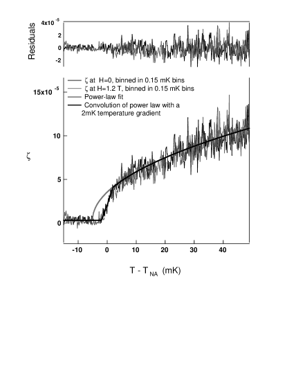
FIG. 1.: Pure 8CB, $d=30\,\mu\mathrm{m}$, $0.59\pm 0.02\mathrm{K}/\mathrm{cm}$. Here, $t_{0}={5.0\pm 0.5\,\mathrm{mK}.\over 307\,\mathrm{K}}=1.6\pm 0.1\times 10^{-5}$. Results are shown with and without an external applied field.

The fluctuation-vs.-temperature profile for 8CB is plotted in Fig. 1 (black data curve). There are three distinct sections to the graph:

1. Smectic: Here, $\zeta=3.1\pm 3.0\times 10^{-6}$, and the smectic fluctuation level is flat and indistinguishable from the shot-noise background.

2. Nematic: The data here fit a power law of the form

   $$w_{0}+w_{1}(T-w_{2})^{w_{3}}$$ (3)

   with $w_{0}=3.1\pm 3.0\times 10^{-6}$, $w_{1}=1.43\pm 0.04\times 10^{-5}$, $w_{2}=5.0\pm 0.5\,\mathrm{mK}$, and $w_{3}=0.50\pm 0.05$. The fit (shown in Fig. 1) was done over the largest temperature range that still kept the residuals (top curve in Fig. 1) flat. $w_{0}$ was held to the smectic level, while $w_{3}$ is the exponent of the power law. $w_{2}$, the divergence point of the power law, is identified with the spinodal temperature $T^{*}$. However, it is a phantom divergence point, as the actual phase transition is located at the interface, i.e., at $T-T_{NA}=0\,\mathrm{mK}$ [12]

3. Interface: Ideally, the interface on Fig. 1 would be a vertical line. However, a temperature gradient normal to the sample plane smears out the interface. Varying temperature moves the position of the interface in the field-of-view, but the magnitude of the smearing is stable to within the statistical errors in the data. In practice, we fit the entire data to a convolution of the power law form in Eq. 3 and a linear temperature gradient. This fit differs from the simple power law fit (also shown) only in the interfacial region. The position of the interface is unambiguously determined by the fit and does NOT coincide with the zero point. The top curve in Fig. 1 shows the residuals for such a fit.

We tested for the effect of sample thickness $d$ on the measurements. We find no systematic dependence on sample thickness for $d>7.5\,\mu\mathrm{m}$. For smaller $d$, we find a marked increase in $t_{0}$, which we ascribe to the effect of a small residual rotation ($\approx 0.2^{\circ}$) between the anchoring direction of the top and bottom plates. The twist created by this rotation is strongest for small $d$. The implications of this will be examined in a longer article [13].

Having established the experimental technique, we first study the critical effects of suppressing director fluctuations with an external magnetic field applied along the easy axis of the nematic. Magnetic-field effects in the nematic phase have been studied in the last two decades [14, 15]. Scale fields to change Landau parameters at the NA transition are large; the mean-field effects of such large fields have been studied by Lelidis and Durand [16]. Recently, Mukhopadhyay et al. [9] have shown that based on the HLM mechanism, one expects modest fields to suppress the director fluctuations that drive a mean-field second-order transition first order. They predict a non-analytic dependence of $t_{0}$ on the field $H$ and a critical field, $H_{c}$, above which the transition is second order. In particular, they predict

$$H_{c}=H_{0}\,t_{0}^{1/2},$$ (4)

where $H_{0}$ is a scale field that depends on known material parameters. For 8CB, $H_{0}\approx 3500\,\mathrm{T}$ and from Fig. 1, $t_{0}=1.6\times 10^{-5}$: this implies a critical field of $H_{c}\approx 10\mathrm{T}$.

The magnetic field effect at the transition was probed with a field that could be varied from $0\,\mathrm{T}$ to $1.5\,\mathrm{T}$. Contrary to initial expectations, no suppression of the fluctuations was seen within $50\,\mathrm{mK}$ of the transition point. Two data curves are shown in Fig. 1. The data curves (black representing zero field, and grey representing measurements at a field of $1.2\,\mathrm{T}$) practically fall on top of each other. Likewise, we see no shift in $t_{0}$.

What do the magnetic field studies on a $0\,$–$1.5\,T$ field tell us about the critical field of $\approx 10\,\mathrm{T}$ predicted via the HLM scenario? A weaker effect implies a larger critical field.

To establish an lower bound for $H_{c}$, we look at the small-$|H|$ limit of the HLM prediction,

$$t_{0}(H)/t_{0}\approx 1-m\,H/H_{c},$$ (5)

where $m=(2.17\pm 0.01)$ is the slope of the linear suppression predicted in Ref. [9]. In our case, our confidence level for $t_{0}$ is roughly $10\%$; i.e., the largest suppression of $t_{0}$ that we would not observe is $t_{0}(H)/t_{0}=0.9$. This puts a lower bound on the value of $H_{c}$. The maximum field used is $H=H_{max}=1.5\,\mathrm{T}$. Thus, for 8CB, we find

$$H_{c} \geq {m\,H\over 1-t_{0}(H)/t_{0}}$$ (6)

$$= {(2.17\pm 0.01)\,1.5\,\mathrm{T}\over 0.9}$$ (7)

$$\approx 33\,\mathrm{T}.$$ (8)

Thus, the lower bound for the critical field in our measurements is three times the predicted value.

We also measured the effect of a magnetic field in two mixtures, 0.18 and 0.41 mole fraction 10CB in 8CB. In neither of these samples do we observe a suppression of fluctuations close to $T_{NA}$.

One might worry about the validity of a null result. We do, however, see the expected non-critical suppression of the fluctuations. We find that this depression falls off quadratically with increasing field:

$$\zeta=\zeta_{0}-g_{H}H^{2}.$$ (9)

This non-critical reduction in the field-effect on approaching $T_{NA}$ reflects quite clearly the fact that the (twist and bend) elastic constants are getting stiffer as one approaches $T_{NA}$. In fact, since the magnetic coherence length is $\xi_{H}={({{K\over\xi}})}^{{{1\over 2}}}{{1\over H}}$, one reasonably expects that the field dependence is always a function of $\xi_{H}$; i.e., the coefficient must obey $g_{H}\propto{{1\over K}}$, where $K$ is a diverging elastic constant. Fitting to the value of $\bar{\nu}=0.5$ that is consistent with other experiments and with our earlier fit in zero field, we find that the data clearly agree with this (see also [13].)

Our second experimental test of the HLM effect was the dependence of $t_{0}$ on the concentration $x$ of 10CB in 8CB, between $x=0$ and $x=0.44$. This dependence has been studied previously by adiabatic calorimetry (Marynissen et al. [17]). Anisimov et al. [7] determined the Landau tricritical point (the LTP is the tricritical point predicted by the de Gennes-McMillan theory) to be at $x^{\star}=0.41$. The resolution in the adiabatic calorimetry is, however, limited to $x>0.3$.[18] To test the HLM theory unambiguously, we extended the range of mixture concentration to $x=0$ (pure 8CB). The non-zero latent heat for $x<x^{\star}\approx 0.41$ implies that their data are inconsistent with the de Gennes-McMillan theory but consistent with the HLM form, which contains a small negative cubic term (with a constant cubic coefficient B) that keeps the latent heat non-zero. In HLM, the effective mean-field Landau free energy is

$$f={{1\over 2}}A|\psi|^{2}-{{1\over 3}}B|\psi|^{3}+{{1\over 4}}C|\psi|^{4}+{{1\over 6}}E|\psi|^{6}$$ (10)

In Ref. [7], the condition for coexistence ($f=0$ and $dF/d\psi=0$) was used to calculate the entropy change $\Delta S=L/T$, in terms of the three Landau parameters $A$, $B$, and $C$. Close to the transition, $A\equiv\alpha t$, where $t$ is the reduced temperature, and $\alpha$ is a constant. The variation of the quartic coefficient near the LTP is modeled by $C=C_{0}(x-x^{\star})$. To make connection with our measurements of $t_{0}$, we calculate $t_{0}\equiv A_{NA}/\alpha$, where $A_{NA}$, the quadratic coefficient at the transition, is a function of $B$, $C$, and $E$.

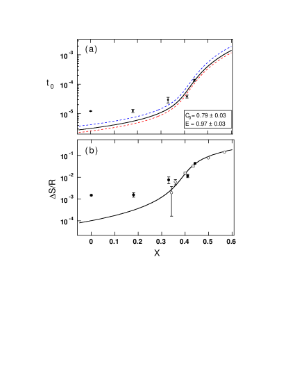
FIG. 2.: (a) Fit of $t_{0}$ data to the Anisimov parameters, with $C_{0}$ as a fit parameter. Top and bottom dashed curves show fits to $t_{0}$ for $\bar{\nu}=0.6$ and $\bar{\nu}=0.4$, respectively. (The data points for these exponent values are not shown.) (b) Comparison of latent heat data (Ref. 16) to $t_{0}$ data (this work). Open circles: data taken from Ref. 16; filled circles: $t_{0}$ data converted to equivalent latent heat.

The fit parameters from the analysis of Anisimov et al. [7] are

$$\beta \equiv -3/8(\alpha C_{0}/E)=0.993$$ (12)

$$\Delta S^{\star}/R=0.0261$$

While the entropy change per mole $\Delta S/R$ depends only on $B$, $\alpha C_{0}$ and $E$, the discontinuity $t_{0}$ depends on all four parameters separately: here, we use the two Anisimov parameters and fit $C_{0}$ and $E$.

Each data point in Fig. 2(a) is obtained from the power-law fit described earlier. The exponent of the power law is fixed at $\bar{\nu}=0.5$. The error bars on a free fit are $\approx 0.1$. In Fig. 2(a) we plot the data for a fitted exponent of $\bar{\nu}=0.5$ and the HLM fit. Also shown, for perspective, are HLM fits for $t_{0}$ data with exponents $\bar{\nu}=0.4$ and $\bar{\nu}=0.6$. The values of $C_{0}$ in the three fits are $-0.74\pm 0.03$, $-0.79\pm 0.03$, and $-0.88\pm 0.03$, respectively. (The best-fit value of $E=0.97\pm 0.03$ for $\bar{\nu}=0.5$ is used for all three fits.) In Fig. 2(b), we compare the latent-heat data of Marynissen et al. [17] with that calculated from our $t_{0}$ data (using the Anisimov parameters). The discontinuity gets larger as we approach the Landau tricritical point. In particular, we find that the data near the LTP agree with the HLM prediction for reasonable values of the quartic coefficient $C_{0}$. However, for lower concentrations of 10CB in 8CB, there is a clear deviation from the HLM prediction, which underestimates the latent heat in this region of the phase diagram [19].

Two main results arise out of this study, and both constrain theories in the weakly type-1 region of the NA transition. The first is the absence of a magnetic field effect on the critical behavior in pure 8CB and in mixtures. It was predicted [9] that an external field would suppress nematic director fluctuations and drive the transition back to second order. Experimentally, we see a non-critical suppression of the fluctuations but observe no change in the critical behavior. In particular, the strength of the first-order transition, measured by the dimensionless number $t_{0}$, is unchanged. We thereby establish a lower bound of $30\,\mathrm{T}$ on the critical magnetic field, three times higher than the predicted value. We conclude that the neglect of smectic fluctuations by HLM is not valid in this region of the phase diagram.

Second, the variation of $t_{0}$ in mixtures has yielded the surprising result that $t_{0}$ on the weakly first-order side of the LTP is larger than the HLM predicted value, and not smaller as one might naively expect of a crossover to second-order XY behavior. This might be related to the observed local maximum in critical exponents seen at the 3DXY to tricritical crossover [4]. This result puts a strong constraint on any theory of the tricritical point.

Both results in this work provide, for the first time, quantitative evidence for deviation from the implications of both the de Gennes-McMillan theory and the HLM theory. Our data show not only that the discontinuity is larger than that predicted by HLM theory but also that the field dependence is much weaker than predicted. These results provide a testing ground for any future theory that goes beyond HLM; the logical next step would be to account for the effect of smectic fluctuations. Future experimental work will focus on the effect of larger fields.

This work was supported by NSERC (Canada). We acknowledge useful discussions with R. Mukhopadhyay and P. Cladis, and thank B. Heinrich for generous access to his magnet.

REFERENCES

- [1] P. Pfeuty and G. Toulouse, Introduction to the Renormalization Group and to Critical Phenomena, 1st ed. (Wiley-Interscience, Chichester, 1978). Cf. p. 153.
- [2] B. I. Halperin, T. C. Lubensky, and S. K. Ma, Phys. Rev. Lett. 32, 292 (1974).
- [3] P. G. de Gennes and J. Prost, The Physics of Liquid Crystals, 2nd ed. (Clarendon Press, Oxford, 1993).
- [4] C. W. Garland and G. Nounesis, Phys. Rev. E 49, 2964 (1994).
- [5] M. A. Anisimov, Mol. Cryst. Liq. Cryst. 162A, 1 (1988)
- [6] P. E. Cladis, in Physical Properties of Liquid Crystals, D. Demus et al., ed., (Wiley-VCH, 1999), pp. 277.
- [7] M. A. Anisimov, P. E. Cladis, E. E. Gorodetskii, D. A. Huse, V. E. Podneks, V. G. Taratuta, W. van Sarloos, and V. P. Voronov, Phys. Rev. A 41, 6749 (1990).
- [8] P. E. Cladis, W. van Sarloos, D. A. Huse, J. S. Patel, J. W. Goodby, and P. L. Finn, Phys. Rev. Lett. 62, 1764 (1989).
- [9] R. Mukhopadhyay, A. Yethiraj, and J. Bechhoefer, Phys. Rev. Lett. (submitted) (1999).
- [10] A. Yethiraj and J. Bechhoefer, Mol. Cryst. Liq. Cryst. 304, 301 (1997).
- [11] A. Yethiraj, Ph.D. thesis, Simon Fraser University, 1999.
- [12] is a phenomenological fit parameter. The real form [13] is more complicated, and the fitted value is merely used to extrapolate data to set .
- [13] A. Yethiraj, R. Mukhopadhyay and J. Bechhoefer, in preparation.
- [14] J. L. Martinand and G. Durand, Sol. St. Commun. 10, 815 (1972).
- [15] Y. Poggi and J. C. Filippini, Phys. Rev. Lett. 39, 150 (1977).
- [16] I. Lelidis and G. Durand, Phys. Rev. Lett. 73, 672 (1994).
- [17] H. Marynissen, J. Thoen, and W. van Dael, Mol. Cryst. Liq. Cryst. 124, 195 (1985).
- [18] The dynamical calorimetry of Ref. [8] extended all the way to pure 8CB; however, the large error bars there limited quantitative comparison with theory.
- [19] One possible explanation for this disagreement is that the linear variation might not be valid; allowing for a nonlinear (quadratic or cubic) correction term in the fit yields a coefficient that is larger than , which is unphysical; this fit is also qualitatively worse (see Ref. [13]).