The temperature dependent bandstructure of a ferromagnetic semiconductor film

Abstract

The electronic quasiparticle spectrum of a ferromagnetic film is investigated within the framework of the s-f model. Starting from the exact solvable case of a single electron in an otherwise empty conduction band being exchange coupled to a ferromagnetically saturated localized spin system we extend the theory to finite temperatures. Our approach is a moment-conserving decoupling procedure for suitable defined Green functions. The theory for finite temperatures evolves continuously from the exact limiting case. The restriction to zero conduction band occupation may be regarded as a proper model description for ferromagnetic semiconductors like EuO and EuS. Evaluating the theory for a simple cubic film cut parallel to the (100) crystal plane, we find some marked correlation effects which depend on the spin of the test electron, on the exchange coupling, and on the temperature of the local-moment system.

I Introduction

Since the mid-70’s there has been a growing theoretical interest in the s-f (or s-d) model [2, 3]. The model works for materials which exhibit local-moment magnetism: for magnetic semiconductors like the europium chalcogenides EuX (X=O, S, Se, Te) [4] and for metallic local-moment systems such as Gd, Tb, and Dy [5]. In the local-moment magnets, the electronic and the magnetic properties are caused by different groups of electrons. Whereas the electronic properties like electrical conductivity are borne by itinerant electrons in rather broad bands, e.g. 6s, 5d for Gd, the magnetism is due to a strongly localized partially filled 4f-shell. In the case of Gd and Eu compounds the 4f-shell is exactly half-filled and, because of Hund’s rules, has its maximal magnetic moment of $S=\frac{7}{2}$.

Many characteristics of the local-moment systems may be explained by a correlation between the localized magnetic states and the itinerant electrons. In the s-f model this correlation is represented by an intra-atomic exchange interaction. The difference between the s-f model and the well-known Kondo lattice model [6] is that in the former the exchange interaction is ferromagnetic, favouring parallel alignment of itinerant electrons and local-moments, whereas in latter it is antiferromagnetic. That is why the s-f model has been recently more and more often referred to as the Ferromagnetic Kondo lattice model [7, 8].

The second aspect of this paper is that of reduced dimensionality. Magnetic phenomena at surfaces and in thin films attract broad attention both theoretically and experimentally due to the question of phase transitions and the variation of magnetic and electronic properties in dimensionally reduced systems [9, 10, 11, 12, 13, 14, 15]. One of the most remarkable examples of the outstanding magnetic properties at surfaces is the existence of magnetically ordered surfaces at temperatures where the bulk material is paramagnetic. This effect has been first documented for Gd(0001) surfaces by Weller et al. [16] and since then been measured by different groups using a wide range of experimental techniques [17, 18, 19]. In these experiments for the difference between the Curie temperature at the surface, $T_{C}({\rm surface})$, and the Curie temperature of bulk Gd, $T_{C}({\rm bulk})$, values between 17K [17] and some 60K [19] have been reported. Succeeding the results for Gd, Tb also was found to have a higher surface Curie temperature, relative to the bulk [20, 21].

Contrary to the groups cited above, Donath et al. [22], using spin-resolved photoemission did not find any indication for an enhanced surface Curie temperature of Gd(0001) surfaces. Other controversially discussed surface properties of Gd include the temperature dependent behaviour of a Gd(0001) surface state [22, 23, 24] which is supposed to play an important role in the interplay between electronic structure and magnetism. A thorough account on the surface magnetism of the lanthanides has been recently given by Dowben et al. [14].

It is not only the dimensionally reduced Gd which is of interest here, even bulk Gd is far from being completely understood. In an earlier study Nolting et al. [25] have predicted that the a priori non-magnetic (5d,6s)-conduction and valence bands should exhibit a marked non-uniform magnetic response at different positions in the Brillouin zone and for different subbands.. Weakly correlated (s-like) dispersions show a Stoner-like $T$-dependence of the exchange splitting. On the other hand, stronger correlated (d-like) dispersions split below $T_{C}$ into four branches, two for each spin direction. Their $T$-dependence mainly concerns the spectral weights of the quasiparticle peaks and not so much the energy positions. Consequently, an exchange caused splitting remains even for $T>T_{c}$. This may be the reason for the fact that the experimental situation is controversial. Kim et al. [26] found a $T$-dependent spin splitting of occupied conduction electron states, which collapses in a Stoner-like fashion for $T\rightarrow T_{C}$. From photoemission experiments, Li et al. [27, 28] conclude that the exchange splitting must be wave-vector dependent, collapsing for some ${\bf k}$ values, while for other no collapse occurs as a function of increasing temperature. This fairly complicated temperature behaviour in the bulk-material must be expected for Gd-films, too.

It is not at all a trivial task to perform an electronic structure calculation for a ferromagnetic local-moment film in such a manner as to realistically incorporate correlation effects. In a previous paper [29] we proposed a simplified model which allowed us to exactly calculate the electronic structure of a model film in the limiting case of ferromagnetic saturation and empty conduction band, $n=0$. This case is applicable to a film of a ferromagnetic semiconductor such as EuO, EuS at $T=0$. Its significance arises from the fact that all relevant correlation effects which are found or expected to occur at finite band occupations and arbitrary temperatures [25, 30, 31], do already appear in this rigorously tractable special case [32, 33].

In this paper we extend the $T=0$ special case to finite temperatures. As a result we will calculate the electronic structure of a local-moment film with a single-electron in an otherwise empty conduction band within the whole temperature range from $T=0$ and $T=T_{c}$.

In the next section we present the model and define the corresponding many-body problem. Subsequently the model is evaluated in two steps, in section II A for the electronic subsystem, and in section II B for the local-moment system. Section III is devoted to a detailed discussion of the results obtained for different film thicknesses and various exchange couplings and temperatures. Comprehensive conclusions with an outlook on the possible application of the model to real substances and on the evaluation of temperature dependent surface states in section IV complete the paper.

II Theoretical Model

We investigate a film consisting of $n$ equivalent layers parallel to the surface of the film. Each lattice site of the film is indicated by a greek letter $\alpha$, $\beta$, $\gamma$, $\ldots$ denoting the layer index and a latin letter $i$, $j$, $k$, $\ldots$ numbering the sites within a given layer. Each layer possesses two-dimensional translational symmetry. Accordingly, the thermodynamic average of any site dependent operator $A_{i\alpha}$ depends only on the layer index $\alpha$:

$$\left\langle A_{i\alpha}\right\rangle\equiv\left\langle A_{\alpha}\right\rangle.$$ (1)

The complete s-f model Hamiltonian

$${\cal H}={\cal H}_{s}+{\cal H}_{f}+{\cal H}_{sf}$$ (2)

consists of three parts. The first

$${\cal H}_{s}=\sum_{ij\alpha\beta}T^{\alpha\beta}_{ij}c^{+}_{i\alpha\sigma}c_{j\beta\sigma}$$ (3)

describes the itinerant conduction electrons as s-electrons. $c^{+}_{i\alpha\sigma}$ and $c_{j\beta\sigma}$ are, respectively the creation and annihilation operators of an electron with the spin $\sigma$ at the lattice site ${\bf R}_{i\alpha}$. $T^{\alpha\beta}_{ij}$ are the hopping integrals.

Each lattice site ${\bf R}_{i\alpha}$ is occupied by a localized magnetic moment, represented by a spin operator ${\bf S}_{i\alpha}$. These localized moments are exchange coupled expressed by the Heisenberg Hamiltonian:

$${\cal H}_{f}=-\sum_{ij\alpha\beta}J^{\alpha\beta}_{ij}{\bf S}_{i\alpha}{\bf S}_{j\beta},$$ (4)

where $J^{\alpha\beta}_{ij}$ are the exchange integrals. The problem with the simple Heisenberg model in the form (4) is that due to the Mermin-Wagner theorem [34] there is no solution showing collective magnetic order at finite temperature, $T>0$. To avoid this obstacle we have chosen an extended Hamiltonian for the localized moments,

$${\cal H}^{*}_{f}={\cal H}_{f}+{\cal H}_{A}={\cal H}_{f}-D_{0}\sum_{i\alpha}(S^{z}_{i\alpha})^{2},$$ (5)

which additionally to the Heisenberg Hamiltonian, ${\cal H}_{f}$ features a single-ion anisotropy term ${\cal H}_{A}$. $D_{0}$ is the according anisotropy constant, which is typically smaller by some orders of magnitude than the Heisenberg exchange interaction, $D_{0}\ll J^{\alpha\beta}_{ij}$.

The distinguishing feature of the s-f model is an intra-atomic exchange between the conduction electrons and the localized f-spins,

$${\cal H}_{sf}=-\frac{J}{\hslash}\sum_{i\alpha}{\bf S}_{i\alpha}\sigma_{i\alpha}$$ (6)

Here, $J$ is the s-f exchange interaction and $\sigma_{i\alpha}$ is the Pauli spin operator of the conduction band electrons. For the materials we are interested in the s-f coupling is positive ($J>0$). In the case where $J<0$ the model Hamiltonian (2) is that of the so-called Kondo lattice. Using the second-quantized form of $\sigma_{i\alpha}$ and the abbreviations

$$S^{\sigma}_{j\beta}=S^{x}_{j\beta}+{\rm i}z_{\sigma}S^{y}_{j\beta};\quad z_{\uparrow(\downarrow)}=\pm 1,$$ (7)

the s-f Hamiltonian can be written as

$${\cal H}_{sf}=-\frac{J}{2}\sum_{i\alpha\sigma}\left(z_{\sigma}S^{z}_{i\alpha}n_{i\alpha\sigma}+S^{\sigma}_{i\alpha}c^{+}_{i\alpha-\sigma}c_{i\alpha\sigma}\right).$$ (8)

The most decisive part of the s-f Hamiltonian (8) is the second term, which describes spin exchange processes between the conduction electrons (3) and the localized moments (4).

In general, the alignment of the localized moments will be influenced by the s-f interaction, which can mediate an indirect interaction (RKKY) via the occupied conduction band [31]. However, here we are interested in the electronic quasiparticle spectrum of a ferromagnetic semiconductor according to a simple test electron in an otherwise empty conduction band. In this case, the localized spin state cannot be affected by the s-f interaction. Furthermore, one knows from experiment that typical Heisenberg exchange integrals are smaller by some orders of magnitudes than their s-f counterparts. In this respect, it seems appropriate to neglect the Heisenberg exchange integrals for the calculation of the electronic properties of the system. Accordingly, the Hamiltonian (2) can be split into an electronic, ${\cal H}_{s}+{\cal H}_{sf}$, and a magnetic part, ${\cal H}^{*}_{f}$, which can be solved separately.

A The electronic subsystem

Starting from the Hamiltonian of the electronic subsystem,

$${\cal H}^{*}={\cal H}_{s}+{\cal H}_{sf},$$ (9)

all physical relevant information of the system can be derived from the retarded single-electron Green function:

$$G^{\alpha\beta}_{ij\sigma}(E) = \left\langle\!\left\langle c_{i\alpha\sigma};c^{+}_{j\beta\sigma}\right\rangle\!\right\rangle_{E}$$ (10)

$$= -{\rm i}\int\limits_{0}^{\infty}dt\>{\rm e}^{-\frac{{\rm i}}{\hslash}Et}\left\langle\left[c_{i\alpha\sigma}(t),c^{+}_{j\beta\sigma}(0)\right]_{+}\right\rangle.$$ (11)

Here and in what follows $[.,.]_{+}$ ($[.,.]_{-}$) is the anticommutator (commutator). Conform to the two-dimensional translational symmetry, we perform a Fourier transformation within the layers of the film,

$$G^{\alpha\beta}_{{\bf k}\sigma}(E)=\frac{1}{N}\sum_{ij}{\rm e}^{{\rm i}{\bf k}({\bf R}_{i}-{\bf R}_{j})}G^{\alpha\beta}_{ij\sigma}(E),$$ (12)

where $N$ is the number of sites per layer, ${\bf k}$ is an in-plane wavevector from the first 2D-Brillouin zone of the layers and ${\bf R}_{i}$ represents the in-plane part of the position vector, ${\bf R}_{i\alpha}={\bf R}_{i}+{\bf r}_{\alpha}$. From Eq. (12) we get the local spectral density by

$$S^{\alpha\beta}_{{\bf k}\sigma}(E)=-\frac{1}{\pi}{\rm Im}G^{\alpha\beta}_{{\bf k}\sigma}(E+{\rm i}0^{+}),$$ (13)

which is directly related to observable quantities within angle and spin resolved direct and inverse photoemission experiments. Finally, the wave-vector summation of $S^{\alpha\beta}_{{\bf k}\sigma}(E)$ yields the layer-dependent (local) quasiparticle density of states:

$$\rho_{\alpha\sigma}(E)=\frac{1}{\hslash N}\sum_{{\bf k}}S^{\alpha\alpha}_{{\bf k}\sigma}(E).$$ (14)

In the following discussion all results will be interpreted in terms of the spectral density (13) and the local density of states (14).

For the solution of the many-body problem posed by Eq. (9) we write down the equation of motion of the single-electron Green function (10)

$$E\,G^{\alpha\beta}_{ij\sigma}=\hslash\delta^{\alpha\beta}_{ij}+\sum_{m\mu}T^{\alpha\mu}_{im}G^{\mu\beta}_{mj\sigma}+\langle\!\langle[c_{i\alpha\sigma},{\cal H}_{sf}]_{-};c^{+}_{j\beta\sigma}\rangle\!\rangle_{E},$$ (15)

where $\delta^{\alpha\beta}_{ij}\equiv\delta_{\alpha\beta}\delta_{ij}$. The formal solution of Eq. (15) can be found by introducing the self-energy $M^{\alpha\beta}_{ij\sigma}(E)$,

$$\left\langle\!\left\langle\left[c_{i\alpha\sigma},{\cal H}_{sf}\right]_{-};c^{+}_{j\beta\sigma}\right\rangle\!\right\rangle_{E}=\sum_{m\mu}M^{\alpha\mu}_{im\sigma}(E)G^{\mu\beta}_{mj\sigma}(E),$$ (16)

which contains all information about the correlations between the conduction band and localized moments. After combining Eqs. (15) and (16) and performing a two-dimensional Fourier transform we see that the formal solution of Eq. (15) is given by

$${\bf G}_{{\bf k}\sigma}(E)=\hslash\left(E\,{\bf I}-{\bf T}_{\bf k}-{\bf M}_{{\bf k}\sigma}(E)\right)^{-1},$$ (17)

where ${\bf I}$ represents the ($n\times n$) identity matrix and where the matrices ${\bf G}_{{\bf k}\sigma}(E)$, ${\bf T}_{\bf k}$, and ${\bf M}_{{\bf k}\sigma}(E)$ have as elements the layer-dependent functions $G^{\alpha\beta}_{{\bf k}\sigma}(E)$, $T^{\alpha\beta}_{{\bf k}}$, and $M^{\alpha\beta}_{{\bf k}\sigma}(E)$, respectively.

To explicitly get the self-energy in Eq. (16) we evaluate the Green function

$$\left\langle\!\left\langle\left[c_{i\alpha\sigma},{\cal H}_{sf}\right]_{-};c^{+}_{j\beta\sigma}\right\rangle\!\right\rangle_{E}=-\frac{J}{2}\left(z_{\sigma}{\it\Gamma}^{\alpha\alpha\beta}_{iij\sigma}+F^{\alpha\alpha\beta}_{iij\sigma}\right).$$ (18)

Here the two higher Green functions,

$${\it\Gamma}^{\alpha\gamma\beta}_{ikj\sigma}(E) = \left\langle\!\left\langle S^{z}_{i\alpha}c_{k\gamma\sigma};c^{+}_{j\beta\sigma}\right\rangle\!\right\rangle_{E},$$ (19)

$$F^{\alpha\alpha\beta}_{iij\sigma}(E) = \left\langle\!\left\langle S^{-\sigma}_{i\alpha}c_{k\gamma-\sigma};c^{+}_{j\beta\sigma}\right\rangle\!\right\rangle_{E},$$ (20)

originate form the two terms of the s-f Hamiltonian (8) and will be referred to as the Ising and the Spin-flip function, respectively. Considering the equations of motion for these two Green functions we encounter the two higher Green functions $\langle\!\langle[S^{z}_{i\alpha}c_{k\gamma\sigma},{\cal H}_{sf}]_{-};c^{+}_{j\beta\sigma}\rangle\!\rangle_{E}$ and $\langle\!\langle[S^{-\sigma}_{i\alpha}c_{k\gamma-\sigma},{\cal H}_{sf}]_{-};c^{+}_{j\beta\sigma}\rangle\!\rangle_{E}$. Since we consider an empty conduction band the thermodynamic average in the Green functions has to be computed with the electron vacuum state $\left|n=0\right\rangle$. From the definition of the s-f Hamiltonian (8) we then see that $\left\langle n=0\right|{\cal H}_{sf}=0$ and, accordingly,

$$\left\langle\!\left\langle\left[S^{z}_{i\alpha},{\cal H}_{sf}\right]_{-}c_{k\gamma\sigma};c^{+}_{j\beta\sigma}\right\rangle\!\right\rangle_{E} \stackrel{{\scriptstyle n\rightarrow 0}}{{\longrightarrow}} 0,$$

$$\left\langle\!\left\langle\left[S^{-\sigma}_{i\alpha},{\cal H}_{sf}\right]_{-}c_{k\gamma-\sigma};c^{+}_{j\beta\sigma}\right\rangle\!\right\rangle_{E} \stackrel{{\scriptstyle n\rightarrow 0}}{{\longrightarrow}} 0.$$

Hence, for the equations of motion of the Ising and the Spin-flip function we get

$$\sum_{m\mu}\left(E\delta^{\gamma\mu}_{km}-T^{\gamma\mu}_{km}\right){\it\Gamma}^{\alpha\mu\beta}_{imj\sigma}(E)$$ (21)

$$= \hslash\left\langle S^{z}_{\alpha}\right\rangle\delta^{\gamma\beta}_{kj}+\left\langle\!\left\langle S^{z}_{i\alpha}\left[c_{k\gamma\sigma},{\cal H}_{sf}\right]_{-};c^{+}_{j\beta\sigma}\right\rangle\!\right\rangle_{E}$$ (22)

$$\sum_{m\mu}\left(E\delta^{\gamma\mu}_{km}-T^{\gamma\mu}_{km}\right)F^{\alpha\mu\beta}_{imj\sigma}(E)$$ (23)

$$= \left\langle\!\left\langle S^{-\sigma}_{i\alpha}\left[c_{k\gamma-\sigma},{\cal H}_{sf}\right]_{-};c^{+}_{j\beta\sigma}\right\rangle\!\right\rangle_{E}.$$ (24)

On the right-hand side of these equations appear further higher Green functions which prevent a direct solution and require an approximative treatment. The treatment is different for the non-diagonal terms, $(i,\alpha)\neq(k,\gamma)$ and for the diagonal terms, $(i,\alpha)=(k,\gamma)$. In the first case we use a self-consistent so-called self-energy approach which results in a decoupling of the equations of motion. For the diagonal terms, $(i,\alpha)=(k,\gamma)$, this approach is replaced by a moment technique which takes the local correlations better into account.

a Non-diagonal terms $(i,\alpha)\neq(k,\gamma)$:

The definition of the self-energy (16) formally corresponds to the substitution

$$\left[c_{i\alpha\sigma},{\cal H}_{sf}\right]_{-}\longrightarrow\sum_{m\mu}M^{\alpha\mu}_{im\sigma}(E)c_{m\mu\sigma}$$ (25)

within the brackets of the Green function. The inspection of the spectral decomposition of the two functions in Eq. (16) reveals that both, $\langle\!\langle[c_{i\alpha\sigma},{\cal H}_{sf}]_{-};c^{+}_{j\beta\sigma}\rangle\!\rangle_{E}$ and $\langle\!\langle c_{i\alpha\sigma};c^{+}_{j\beta\sigma}\rangle\!\rangle_{E}$, have the same pole structure and can differ only by the spectral weights of their poles. The equality of both sides in Eq. (16) is installed by the self-energy components $M^{\alpha\beta}_{ij\sigma}(E)$. Inspecting now the spectral representations of the two Green functions $\langle\!\langle S^{-\sigma}_{i\alpha}[c_{k\gamma\sigma},{\cal H}_{sf}]_{-};c^{+}_{j\beta\sigma}\rangle\!\rangle_{E}$ and $\langle\!\langle S^{-\sigma}_{i\alpha}c_{k\gamma\sigma};c^{+}_{j\beta\sigma}\rangle\!\rangle_{E}$ we notice that the additional spin operator $S^{-\sigma}_{i\alpha}$ selects for both only those poles of the original Green functions without spin operator which are connected with a spin-flip of the electron. Hence, the poles of these two functions build subset of the poles of the two Green functions from Eq. (16) and are, therefore, identical to each other. Again, only the weights of the poles can differ. In analogy to Eqs. (16) and (25) we now propose to use the plausible ansatz

$$\left\langle\!\left\langle S^{-\sigma}_{i\alpha}\left[c_{k\gamma-\sigma},{\cal H}_{sf}\right]_{-};c^{+}_{j\beta\sigma}\right\rangle\!\right\rangle_{E}$$ (27)

$$\approx\sum_{m\mu}M^{\gamma\mu}_{km-\sigma}(E)\left\langle\!\left\langle S^{-\sigma}_{i\alpha}c_{m\mu-\sigma};c^{+}_{j\beta\sigma}\right\rangle\!\right\rangle_{E}.$$

A similar reasoning can be used for:

$$\left\langle\!\left\langle S^{z}_{i\alpha}\left[c_{k\gamma\sigma},{\cal H}_{sf}\right]_{-};c^{+}_{j\beta\sigma}\right\rangle\!\right\rangle_{E}$$ (29)

$$\approx\sum_{m\mu}M^{\gamma\mu}_{km\sigma}(E)\left\langle\!\left\langle S^{z}_{i\alpha}c_{m\mu\sigma};c^{+}_{j\beta\sigma}\right\rangle\!\right\rangle_{E},$$

with the difference that here the additional spin operator $S^{z}_{i\alpha}$ does not change the original pole structure but merely modifies the spectral weights of the poles. On the right-hand sides of Eqs. (27) and (29) we find the already known Spin-flip and Ising function, respectively. Hence, for $(i,\alpha)\neq(k,\gamma)$, the Eqs. (15), (18), (21), (23), (27), and (29) build a closed system .

b Diagonal elements $(i,\alpha)=(k,\gamma)$:

We start with the explicit evaluation of the higher Green functions on the right-hand sides of Eqs. (21) and (23). For Eq. (23) we get, for $(i,\alpha)=(k,\gamma)$,

$$\left\langle\!\left\langle S^{-\sigma}_{i\alpha}\left[c_{i\alpha-\sigma},{\cal H}_{sf}\right]_{-};c^{+}_{j\beta\sigma}\right\rangle\!\right\rangle_{E}$$ (31)

$$=\frac{J}{2}\left(z_{\sigma}\dot{F}^{\alpha\alpha\beta}_{iij\sigma}(E)-\ddot{F}^{\alpha\alpha\beta}_{iij\sigma}(E)\right),$$

where we have abbreviated

$$\dot{F}^{\alpha\alpha\beta}_{iij\sigma}(E) = \left\langle\!\left\langle S^{-\sigma}_{i\alpha}S^{z}_{i\alpha}c_{i\alpha-\sigma};c^{+}_{j\beta\sigma}\right\rangle\!\right\rangle_{E},$$ (33)

$$\ddot{F}^{\alpha\alpha\beta}_{iij\sigma}(E) = \left\langle\!\left\langle S^{-\sigma}_{i\alpha}S^{\sigma}_{i\alpha}c_{i\alpha\sigma};c^{+}_{j\beta\sigma}\right\rangle\!\right\rangle_{E}.$$ (34)

The analogous evaluation of the higher Green function in Eq. (21) does not require any further higher Green functions, because it can be expressed in terms of already known Green functions:

$$\!\!\langle\!\langle S^{z}_{i\alpha}[c_{i\alpha\sigma},{\cal H}_{sf}]_{-};c^{+}_{j\beta\sigma}\rangle\!\rangle_{E}\!+\!z_{\sigma}\langle\!\langle S^{-\sigma}_{i\alpha}[c_{i\alpha-\sigma},{\cal H}_{sf}]_{-};c^{+}_{j\beta\sigma}\rangle\!\rangle_{E}$$ (35)

$$= \frac{J\hslash}{2}({\it\Gamma}^{\alpha\alpha\beta}_{iij\sigma}(E)+z_{\sigma}F^{\alpha\alpha\beta}_{iij\sigma}(E)-z_{\sigma}\hslash S(S+1)G^{\alpha\beta}_{ij\sigma}(E)).$$ (36)

As Eq. (31), the above relation is still exact. To get a close system of equations we are left with the determination of the functions $\dot{F}^{\alpha\alpha\beta}_{iij\sigma}(E)$ and $\ddot{F}^{\alpha\alpha\beta}_{iij\sigma}(E)$. Both fulfil exact relations which will be used to derive satisfying approximations. For spin $S=\frac{1}{2}$ we find for all temperatures:

$$\dot{F}^{\alpha\alpha\beta}_{iij\sigma}(E)\Big{|}_{S=\frac{1}{2}} = {\textstyle\frac{1}{2}}z_{\sigma}\hslash F^{\alpha\alpha\beta}_{iij\sigma}(E),$$ (39)

$$\ddot{F}^{\alpha\alpha\beta}_{iij\sigma}(E)\Big{|}_{S=\frac{1}{2}} = {\textstyle\frac{1}{2}}\hslash^{2}G^{\alpha\beta}_{ij\sigma}(E)-z_{\sigma}\hslash{\it\Gamma}^{\alpha\alpha\beta}_{iij\sigma}(E).$$ (40)

On the other hand, in the case of ferromagnetic saturation, $\langle S^{z}_{\alpha}\rangle\equiv S$, it holds for arbitrary spin:

$$\dot{F}^{\alpha\alpha\beta}_{iij\sigma}(E)\Big{|}_{T=0} = \hslash\left((S-{\textstyle\frac{1}{2}})+{\textstyle\frac{1}{2}}z_{\sigma}\right)F^{\alpha\alpha\beta}_{iij\sigma}(E),$$ (42)

$$\ddot{F}^{\alpha\alpha\beta}_{iij\sigma}(E)\Big{|}_{T=0} = \hslash^{2}SG^{\alpha\beta}_{ij\sigma}(E)-z_{\sigma}\hslash{\it\Gamma}^{\alpha\alpha\beta}_{iij\sigma}(E).$$ (43)

The exact limiting cases (b) and (b) suggest the general structures:

$$\dot{F}^{\alpha\alpha\beta}_{iij\sigma}(E) = \kappa^{(1)}_{\alpha\sigma}G^{\alpha\beta}_{ij\sigma}(E)+\lambda^{(1)}_{\alpha\sigma}F^{\alpha\alpha\beta}_{iij\sigma}(E),$$ (45)

$$\ddot{F}^{\alpha\alpha\beta}_{iij\sigma}(E) = \kappa^{(2)}_{\alpha\sigma}G^{\alpha\beta}_{ij\sigma}(E)+\lambda^{(2)}_{\alpha\sigma}{\it\Gamma}^{\alpha\alpha\beta}_{iij\sigma}(E).$$ (46)

For the five Green functions of the type $\langle\!\langle A;B\rangle\!\rangle_{E}$ in Eqs. (b) we can calculate the spectral moments,

$$M^{(n)}_{AB}=\left\langle\left({\rm i}\hslash\frac{\partial}{\partial t}\right)^{n}\left[A(t),B(0)\right]_{+}\right\rangle_{t=0},$$ (47)

where $n=1,2,\ldots$ . Because of the equivalent relation

$$M^{(n)}_{AB}=-\frac{1}{\pi\hslash}\int\limits_{-\infty}^{\infty}dE\>E^{n}{\rm Im}\left\langle\!\left\langle A;B\right\rangle\!\right\rangle_{E},$$ (48)

the moments can be used to fix the coefficients $\kappa^{(m)}_{\alpha\sigma}$ and $\lambda^{(m)}_{\alpha\sigma}$ in Eqs. (b). After tedious but straightforward calculations, we get

$$\kappa^{(1)}_{\alpha\sigma}=0,\quad\kappa^{(2)}_{\alpha\sigma}=\langle S^{-\sigma}_{\alpha}S^{\sigma}_{\alpha}\rangle-\lambda^{(2)}_{\alpha\sigma}\langle S^{z}_{\alpha}\rangle,$$ (49)

$$\lambda^{(1)}_{\alpha\sigma}=\displaystyle\frac{\langle S^{-\sigma}_{\alpha}S^{\sigma}_{\alpha}S^{z}_{\alpha}\rangle+z_{\sigma}\langle S^{-\sigma}_{\alpha}S^{\sigma}_{\alpha}\rangle}{\langle S^{-\sigma}_{\alpha}S^{\sigma}_{\alpha}\rangle},$$ (50)

$$\lambda^{(2)}_{\alpha\sigma}=\displaystyle\frac{\langle S^{-\sigma}_{\alpha}S^{\sigma}_{\alpha}S^{z}_{\alpha}\rangle-\langle S^{z}_{\alpha}\rangle\langle S^{-\sigma}_{\alpha}S^{\sigma}_{\alpha}\rangle}{\langle(S^{z}_{\alpha})^{2}\rangle-\langle S^{z}_{\alpha}\rangle^{2}}.$$ (51)

The coefficients are determined by f-spin correlation functions, which will be determined at a later stage.

The Eqs. (15), (18), (21), (23), (27)–(31), (35), (b), and (49) represent a closed system, which can be solved self-consistently. Before proceeding we assume that the self-energy from Eq. (16) is a local entity

$$M^{\alpha\beta}_{{\bf k}\sigma}(E)\equiv\delta_{\alpha\beta}M^{\alpha}_{\sigma}(E).$$ (52)

The reason for the ${\bf k}$ independence can be traced back to the neglect of magnon energies [30]. The restriction to the diagonal elements in the greek indices denoting the layers is in that sense the transfer of the ${\bf k}$ independence in the case of three dimensions [30] to the film geometries discussed in this paper. Furthermore one can show that the assumption (52) is not necessary for the following calculations but merely drastically simplifies them.

We can now use Eqs. (27)–(31), (35), (b), and (49) to evaluate the Ising and the Spin-flip functions in Eqs. (21) and (23). As the result we get the Fourier transformed Ising and Spin-flip functions. According to Eq. (18) we can restrict our attention to the diagonal elements ${\it\Gamma}^{\alpha\alpha\beta}_{{\bf kq}\sigma}(E)$ and $F^{\alpha\alpha\beta}_{{\bf kq}\sigma}(E)$. After subsequent ${\bf q}$-summation we eventually get, using Eqs. (17) and (52):

$$\hslash\sum_{{\bf q}}{\it\Gamma}^{\alpha\alpha\beta}_{{\bf kq}\sigma} = \sqrt{N}\hslash\langle S^{z}_{\alpha}\rangle G^{\alpha\beta}_{{\bf k}\sigma}-G^{\alpha\alpha}_{{\bf 0}\sigma}\Big{\{}M^{\alpha}_{\sigma}\sum_{{\bf q}}{\it\Gamma}^{\alpha\alpha\beta}_{{\bf kq}\sigma}$$ (57)

$$-\frac{J}{2}\Big{(}z_{\sigma}(\kappa^{(2)}_{\alpha\sigma}-\hslash^{2}S(S+1))\sqrt{N}G^{\alpha\beta}_{{\bf k}\sigma}$$

$$+(z_{\sigma}\hslash-\lambda^{(1)}_{\alpha\sigma})\sum_{{\bf q}}F^{\alpha\alpha\beta}_{{\bf kq}\sigma}$$

$$+(\hslash+z_{\sigma}\lambda^{(2)}_{\alpha\sigma})\sum_{{\bf q}}{\it\Gamma}^{\alpha\alpha\beta}_{{\bf kq}\sigma}\Big{)}\Big{\}},$$

$$\hslash\sum_{{\bf q}}F^{\alpha\alpha\beta}_{{\bf kq}\sigma} = -G^{\alpha\alpha}_{{\bf 0}-\sigma}\Big{\{}M^{\alpha}_{-\sigma}\sum_{{\bf q}}F^{\alpha\alpha\beta}_{{\bf kq}\sigma}+\frac{J}{2}\Big{(}\kappa^{(2)}_{\alpha\sigma}\sqrt{N}G^{\alpha\beta}_{{\bf k}\sigma}$$ (59)

$$-z_{\sigma}\lambda^{(1)}_{\alpha\sigma}\sum_{{\bf q}}F^{\alpha\alpha\beta}_{{\bf kq}\sigma}+\lambda^{(2)}_{\alpha\sigma}\sum_{{\bf q}}{\it\Gamma}^{\alpha\alpha\beta}_{{\bf kq}\sigma}\Big{)}\Big{\}},$$

where we have introduced

$$G^{\alpha\alpha}_{{\bf 0}\sigma}(E)=\frac{1}{N}\sum_{{\bf k}}G^{\alpha\alpha}_{{\bf k}\sigma}(E).$$ (60)

The set of equations (b) can be solved to express the sums $\sum_{{\bf q}}{\it\Gamma}^{\alpha\alpha\beta}_{{\bf kq}\sigma}(E)$ and $\sum_{{\bf q}}F^{\alpha\alpha\beta}_{{\bf kq}\sigma}(E)$ in terms of the single-electron Green function $G^{\alpha\beta}_{{\bf k}\sigma}(E)$. However, by inspecting Eqs. (b) we see that these expressions will still contain the layer and spin-dependent self-energy $M^{\alpha}_{\sigma}(E)$.

To solve this problem we combine Eqs. (16) and (18) and get, after Fourier transformation:

$$M^{\alpha}_{\sigma}G^{\alpha\beta}_{{\bf k}\sigma}=-\frac{J}{2\sqrt{N}}\left(z_{\sigma}\sum_{{\bf q}}{\it\Gamma}^{\alpha\alpha\beta}_{{\bf kq}\sigma}+\sum_{{\bf q}}F^{\alpha\alpha\beta}_{{\bf kq}\sigma}\right).$$ (61)

Combining this equation with the results obtained for $\sum_{{\bf q}}{\it\Gamma}^{\alpha\alpha\beta}_{{\bf kq}\sigma}(E)$ and $\sum_{{\bf q}}F^{\alpha\alpha\beta}_{{\bf kq}\sigma}(E)$ from Eqs. (b) we eventually get an implicit set of equations for the layer and spin-dependent electronic self-energy:

$$M^{\alpha}_{\sigma}(E)=-\frac{J}{2}m^{\alpha}_{\sigma}(E),\quad m^{\alpha}_{\sigma}(E)=\frac{Z^{\alpha}_{\sigma}(E)}{N^{\alpha}_{\sigma}(E)},$$ (62)

where the numerator and the denominator, respectively, are given by

$$Z^{\alpha}_{\sigma} = z_{\sigma}\hslash^{2}\langle S^{z}_{\alpha}\rangle+\frac{J}{2}\Big{\{}\big{(}\kappa^{(2)}_{\alpha\sigma}-\hslash^{2}S(S+1)\big{)}G^{\alpha\alpha}_{{\bf 0}\sigma}$$ (67)

$$-\big{(}(\lambda^{(1)}_{\alpha\sigma}+\lambda^{(2)}_{\alpha\sigma}+z_{\sigma}m^{\alpha}_{-\sigma})\hslash\langle S^{z}_{\alpha}\rangle+\hslash\kappa^{(2)}_{\alpha\sigma}\big{)}G^{\alpha\alpha}_{{\bf 0}-\sigma}\Big{\}}$$

$$+\frac{J^{2}}{4}\Big{\{}z_{\sigma}\hslash^{2}S(S+1)(\lambda^{(1)}_{\alpha\sigma}+\lambda^{(2)}_{\alpha\sigma}+z_{\sigma}m^{\alpha}_{-\sigma})$$

$$+\kappa^{(2)}_{\alpha\sigma}(m^{\alpha}_{\sigma}-m^{\alpha}_{-\sigma})\Big{\}}G^{\alpha\alpha}_{{\bf 0}\sigma}G^{\alpha\alpha}_{{\bf 0}-\sigma},$$

$$N^{\alpha}_{\sigma} = \hslash^{2}-\frac{J}{2}\Big{\{}(\hslash+z_{\sigma}\lambda^{(2)}_{\alpha\sigma}+m^{\alpha}_{\sigma})G^{\alpha\alpha}_{{\bf 0}\sigma}+(z_{\sigma}\lambda^{(1)}_{\alpha\sigma}$$ (70)

$$+m^{\alpha}_{-\sigma})G^{\alpha\alpha}_{{\bf 0}-\sigma}\Big{\}}+\frac{J^{2}}{4}\Big{\{}(m^{\alpha}_{\sigma}+\hslash)(m^{\alpha}_{-\sigma}+z_{\sigma}\lambda^{(1)}_{\alpha\sigma})$$

$$+z_{\sigma}\lambda^{(2)}_{\alpha\sigma}(m^{\alpha}_{-\sigma}+\hslash)\Big{\}}G^{\alpha\alpha}_{{\bf 0}\sigma}G^{\alpha\alpha}_{{\bf 0}-\sigma}.$$

The implicit set of equations (62) and (62) now enables us to self-consistently evaluate the self-energy of the system provided that the f-spin correlation functions from Eqs. (49) are known. These will be evaluated in the next section.

B The local-moment system

The system of localized f-moments is described by the extended Heisenberg Hamiltonian (5) which we write down again for convenience:

$${\cal H}^{*}_{f}=-\sum_{ij\alpha\beta}J^{\alpha\beta}_{ij}{\bf S}_{i\alpha}{\bf S}_{j\beta}-D_{0}\sum_{i\alpha}(S^{z}_{i\alpha})^{2}.$$ (71)

Here we want to stress once more that the single-ion anisotropy constant $D_{0}$ is small compared to the Heisenberg exchange interaction, $D_{0}\ll J^{\alpha\beta}_{ij}$. By defining the magnon Green function

$$D^{\alpha\beta}_{ij}(E)=\left\langle\!\left\langle S^{+}_{i\alpha};S^{-}_{j\beta}\right\rangle\!\right\rangle_{E},$$ (72)

we can calculate the f-spin correlation functions by evaluating the equation of motion

$$E\,D^{\alpha\beta}_{ij}(E)=2\hslash^{2}\delta_{\alpha\beta}\langle S^{z}_{\alpha}\rangle+\left\langle\!\left\langle\left[S^{+}_{i\alpha},{\cal H}^{*}_{f}\right]_{-};S^{-}_{j\beta}\right\rangle\!\right\rangle_{E}.$$ (73)

The evaluation of this equation of motion involves the decoupling of the higher Green functions on its right-hand side, originating from the Heisenberg term. ${\cal H}_{f}$, and the anisotropy term, ${\cal H}_{A}$, using the Random Phase Approximation (RPA) and a decoupling proposed by Lines [35], respectively. The details of the calculation can be found in a previous paper [36]. For brevity we restrict ourselves to present here only the results. For the layer-dependent magnetizations of the f-spin system we get

$$\frac{\langle S^{z}_{\alpha}\rangle}{\hslash}=\frac{(1+\varphi_{\alpha})^{2S+1}(S-\varphi_{\alpha})+\varphi^{2S+1}_{\alpha}(S+1+\varphi_{\alpha})}{\varphi^{2S+1}_{\alpha}-(1+\varphi_{\alpha})^{2S+1}},$$ (74)

where

$$\varphi_{\alpha}=\frac{1}{N}\sum_{{\bf k}}\sum_{\gamma}\frac{\chi_{\alpha\alpha\gamma}({\bf k})}{{\rm e}^{\beta E_{\gamma}({\bf k})}-1},$$ (75)

where, again, $N$ is the number of sites per layer and $\beta=\frac{1}{k_{{\rm B}}T}$. The summation $\sum_{\gamma}$ in Eq. (75) runs over the $n$ poles $E_{\gamma}({\bf k})$ of the Green function $D^{\alpha\beta}_{{\bf k}}(E)$ and the $\chi_{\alpha\alpha\gamma}({\bf k})$ is the weight of the $\gamma$’th pole in the diagonal element of the Green function $D^{\alpha\alpha}_{{\bf k}}(E)$. The poles and the weights can be calculated from the solution of Eq. (73):

$$D^{\alpha\beta}_{{\bf k}}(E)=2\hslash^{2}\left(\begin{array}[]{ccc}\langle S^{z}_{1}\rangle&&0\\ &\ddots&\\ 0&&\langle S^{z}_{n}\rangle\end{array}\right)\cdot(E\,{\bf I}-{\bf A})^{-1},$$ (76)

with

$$\frac{({\bf A})^{\alpha\beta}}{\hslash}=\big{(}D_{0}\Phi_{\alpha}+2\sum_{\gamma}J^{\alpha\gamma}_{{\bf 0}}\langle S^{z}_{\gamma}\rangle\big{)}\delta_{\alpha\beta}-2J^{\alpha\beta}_{{\bf k}}\langle S^{z}_{\alpha}\rangle.$$ (77)

The $\Phi_{\alpha}$ come from the decoupling of the higher Green function on the right-hand side of Eq. (73) which originates from the anisotropy Hamiltonian ${\cal H}_{A}$ according to Lines [35, 36] and are given by:

$$\Phi_{\alpha}=\frac{2\hslash^{2}S(S+1)-3\hslash\langle S^{z}_{\alpha}\rangle(1+2\varphi_{\alpha})}{\langle S^{z}_{\alpha}\rangle}.$$ (78)

Having obtained the layer-dependent magnetizations (74) and the $\varphi_{\alpha}$ we can now express all the other f-spin correlation functions appearing in Eqs. (49) via the relations

$$\langle S^{-}_{\alpha}S^{+}_{\alpha}\rangle = 2\hslash\langle S^{z}_{\alpha}\rangle\varphi_{\alpha},$$ (80)

$$\langle(S^{z}_{\alpha})^{2}\rangle = \hslash^{2}S(S+1)\langle S^{z}_{\alpha}\rangle(1+2\varphi_{\alpha}),$$ (81)

$$\langle(S^{z}_{\alpha})^{3}\rangle = \hslash^{3}S(S+1)\varphi_{\alpha}+\hslash^{2}\langle S^{z}_{\alpha}\rangle\big{(}S(S+1)+\varphi_{\alpha}\big{)}$$ (83)

$$-\hslash\langle(S^{z}_{\alpha})^{2}\rangle(1+2\varphi_{\alpha}),$$

and the general spin-operator equality

$$S^{\sigma}_{i\alpha}S^{-\sigma}_{i\alpha}=\hslash^{2}S(S+1)+z_{\sigma}\hslash S^{z}_{i\alpha}-(S^{z}_{i\alpha})^{2}.$$ (84)

Mediated by Eqs. (49), (62), and (62), the f-spin correlation functions contain the whole temperature dependence of the electronic subsystem (9).

III Results

We have evaluated our theory for a film with simple cubic (s.c.) structure consisting of $n$ layers parallel to the (100)-plane of the crystal. The electron hopping and the Heisenberg exchange integrals shall be restricted within a tight-binding approximation to nearest neighbour coupling,

$$T^{\alpha\beta}_{ij} = \delta^{\alpha\beta}_{i,j+\Delta}T^{\alpha\alpha}+\delta^{\alpha,\beta\pm 1}_{ij}T^{\alpha\beta},$$ (85)

$$J^{\alpha\beta}_{ij} = \delta^{\alpha\beta}_{i,j+\Delta}J^{\alpha\alpha}+\delta^{\alpha,\beta\pm 1}_{ij}J^{\alpha\beta},$$ (86)

respectively. Here $\Delta$ denotes the relative positions of nearest neighbours, both within the same layer, for s.c.(100): $\Delta=(0,1),(0,\bar{1}),(1,0),(\bar{1},0)$. $T^{\alpha\beta}$ is the hopping between the layers $\alpha$ and $\beta=\alpha\pm 1$ and $J^{\alpha\alpha}$ is the exchange interaction within the layer $\alpha$. For the following discussion, furthermore the hopping integrals and the exchange interaction have been assumed to be uniform within the whole film,

$$T^{\alpha\alpha}=T^{\alpha\beta}\equiv T,\quad J^{\alpha\alpha}=J^{\alpha\beta}\equiv J_{ff},$$ (87)

where $J_{ff}$ should not be mixed up with the s-f exchange interaction $J$. For explicit values we choose $T=-0.1$eV, $J_{ff}=0.01$eV, and the single-ion anisotropy $D_{0}/J_{ff}=0.01$.

A f-spin correlation functions

Before we can start calculating the electronic excitation spectra, we first have to evaluate the local-moment system considered in Sec. II B.

FIG. 1.: Layer-dependent magnetizations $\langle S^{z}_{\alpha}\rangle$ of a 20-layer s.c.(100) film for the layers $\alpha=1,2,\ldots,10$. The magnetizations increase from the surface layer towards the center of the film. Inset: Dependence of the Curie temperature $T_{C}$ on the film thickness $n$ of s.c.-(100) films.

FIG. 2.: The different f-spin correlation functions from Eqs. (49) calculated for the centre layers ($\alpha=10,11$) of the 20-layer-film from Fig. 1.

For example, Fig. 1 shows the layer-dependent magnetizations of a 20-layer s.c.(100) film as a function of temperature. As for all other film thicknesses the layer-dependent magnetizations $\langle S^{z}_{\alpha}\rangle$ increase from the surface layers ($\alpha=1,20$) towards the center layers ($\alpha=10,11$) of the film. The inset of Fig. 1 displays dependence of the Curie temperature on the film thickness $n$. The complete set of f-spin correlation functions according to Eqs. (74), (75), (II B), and (84) calculated for the center layer of the 20-layer film can be seen in Fig. 2.

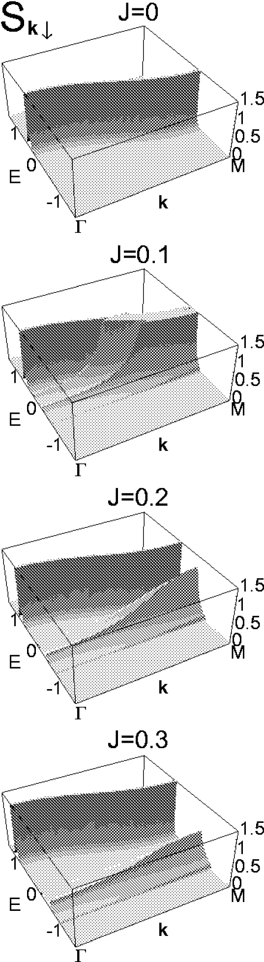
FIG. 3.: Spectral density $S_{{\bf k}\downarrow}(E)$ of a s.c.-(100)-monolayer for ferromagnetic saturation of the local-moment system ($T=0$, $\langle S_{z}\rangle=S$) as a function of energy and wavevector from $\Gamma=(0,0)$ to ${\rm M}=(\pi,\pi)$ for $T=0$ and different values of the s-f exchange interaction $J$.

B The temperature-dependent electronic structure

We discuss our results in terms of the spectral density $S^{\alpha\alpha}_{{\bf k}\sigma}(E)$, defined in Eq. (13), and the local quasiparticle density of states, Eq. (14). We start our discussion of the temperature dependent electronic bandstructure with a special limiting case which gives us an insight into the underlying physics of the problem. The special limiting case of ferromagnetic saturation, $T=0$, and empty conduction band, $n=0$, is exactly solvable, both, for the bulk material [32, 33, 30] and for film geometries [29]. The limiting case, therefore, provides a good testing ground for the theory for finite temperatures presented in Sec. II A.

It turns out that for $T=0$ the $\sigma=\uparrow$-spectrum is rather simple, since a $\uparrow$-electron has no chance to exchange its spin with the ferromagnetically saturated localized f-spin system. The quasiparticle bandstructure is therefore identical to the free Bloch dispersion, only rigidly shifted by a constant energy amount of $-\frac{1}{2}JS$, due to the first Ising-like term in the s-f Hamiltonian (8).

Fig. 3 shows the spin-$\downarrow$ spectral density of a s.c.-(100)-monolayer for the special case of ferromagnetic saturation, $T=0$, for different s-f interactions $J$. For $J=0$ the spectral density represents a $\delta$-function located at the point of the free two-dimensional Bloch dispersion. For small s-f exchange coupling, $J>0$, a slight deformation of the original Bloch dispersion sets in and the quasiparticle peaks get a finite width indicating a finite lifetime. For intermediate and strong couplings the spectral density splits into two parts corresponding to two different spin exchange processes between the excited spin-$\downarrow$ electron and the localized f-spin system. The higher energetic part of the spectrum represents a polarization of the immediate spin neighbourhood of the electron due to a repeated emission and reabsorption of magnons. The result is a polaron-like quasiparticle called the magnetic polaron. The low-energetic part of the spectrum is a scattering band which corresponds to the simple emission of a magnon by the spin-$\downarrow$ electron, which is necessarily connected with a spin-flip of the electron [29].

FIG. 4.: Density of states $\rho_{\downarrow}(E)$ of a s.c.-(100)-monolayer for $T=0$ and for different s-f interactions $J$.

From the spectral density of Fig. 3 we get, using Eq. (14), the local quasiparticle density of states $\rho_{\downarrow}(E)$ of a monolayer, displayed in Fig. 4. Here we see that the splitting of the spectral density discussed above transfers itself to the quasiparticle density of states as a gap for $J\gtrapprox 0.2$. As for the spectral density, the density of states of the spin-$\uparrow$ electron is only rigidly shifted and therefore not displayed.

However, this does not hold any longer for finite temperatures, $T>0$. Fig. 5 exhibits the density of states of a s.c.-(100)-monolayer for different s-f interactions and different temperatures. The dotted lines represent the case of vanishing s-f exchange, $J=0$, where spin-$\downarrow$ and spin-$\uparrow$ spectra are equal. Since the electrons are not coupled to the local-moment system, we also have no temperature dependence. For finite s-f interaction we see from Fig. 4 that in the spin-$\downarrow$ density of states spectral weight is transferred from the high-energetic polaron peak to the low-energetic scattering peak. To explain this effect we have to consider the elementary processes which build the spectrum. The low-energetic scattering peak of the spin-$\downarrow$ electron consists of two elementary processes.

FIG. 5.: Density of states $\rho_{\sigma}(E)$ of a s.c.-(100)-monolayer for different s-f interactions $J$ and different temperatures $T$ (in units of $T_{C}$). The dotted lines represent the case of $J=0$ where there is no distinction between spin-$\downarrow$ and spin-$\uparrow$ electron, $\rho_{\downarrow}(E)=\rho_{\uparrow}(E)$.

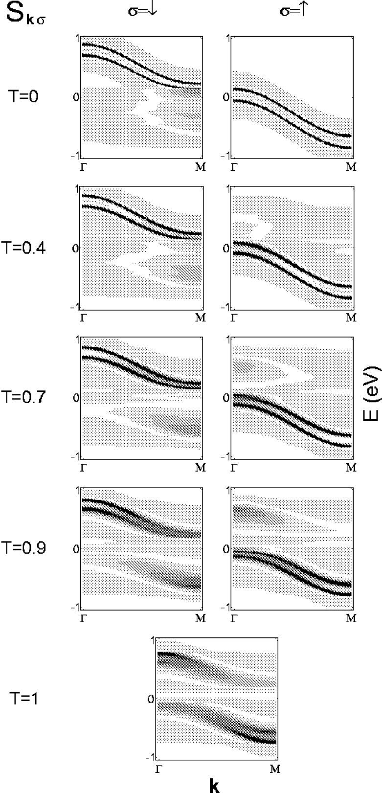
FIG. 6.: Spectral density, $S_{{\bf k}\sigma}(E)=S^{11}_{{\bf k}\sigma}(E)=S^{22}_{{\bf k}\sigma}(E)$, of a s.c.-(100) double-layer as a function of energy and wavevector from $\Gamma=(0,0)$ to $M=(\pi,\pi)$ for $J=0.2$eV and different temperatures $T$ (in units of $T_{C}$).

Because of finite deviation of the f-spin system from saturation for $T>0$, the $\downarrow$-electron has a finite probability of entering the local frame as spin-$\uparrow$ electron. This probability is zero for $\langle S_{z}\rangle=S$ ($T=0$) and increases with increasing temperature. On the other hand, the spin-$\downarrow$ electron can first emit a magnon and by that process reverse its spin, becoming a spin-$\uparrow$ electron in the external frame of coordinates. The spectral weight produced by the first elementary process reduces the spectral weight of the high-energetic polaron peak therefore shifting spectral weight from the high-energetic polaron peaks towards the low-energetic scattering peak.

For the spin-$\uparrow$ electron we see from Fig. 5 that for finite temperatures an additional peak rises at the high-energetic side of the spectra with increasing temperature. We can explain this effect by the spin-$\uparrow$ electron absorbing a magnon and subsequently, as spin-$\downarrow$ electron forming a polaron. Here the magnon absorption by a spin-$\uparrow$ electron is equivalent to the magnon emission by a spin-$\downarrow$ electron. In the case of ferromagnetic saturation the system does not contain any magnons, which is the reason why there is no scattering peak in the spin-$\uparrow$ spectrum at $T=0$. As a result of the shifting of spectral weights towards lower energies for the spin-$\downarrow$ electron and towards higher energies for the spin-$\uparrow$ electron the densities of states for the two spin directions approach each other with increasing temperature.

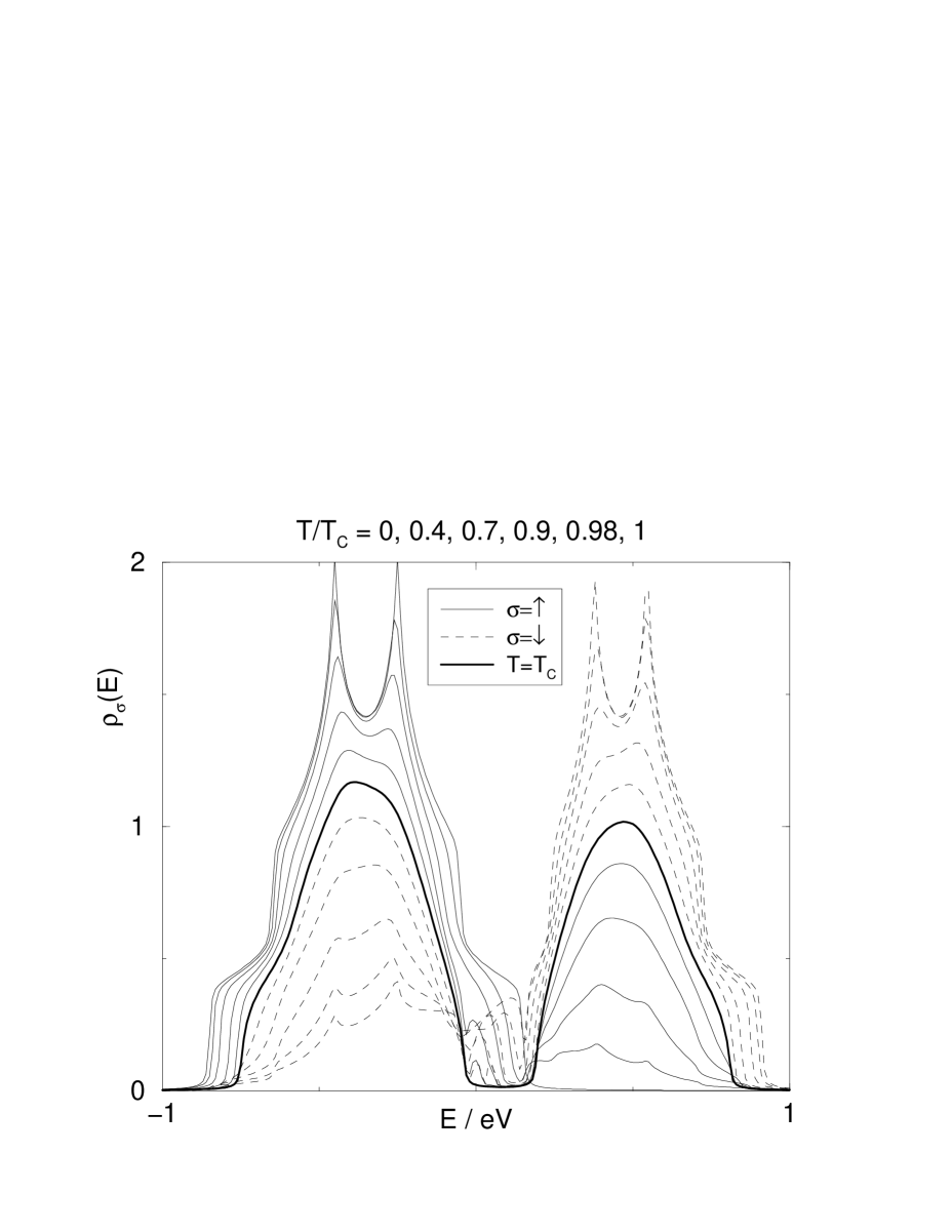
FIG. 7.: Density of states, $\rho_{\sigma}(E)=\rho^{1}_{\sigma}(E)=\rho^{2}_{\sigma}(E)$, of a s.c.-(100) double-layer for $J=0.2$ and different temperatures $T$ (in units of $T_{C}$). The curves for $T=0$ are furthest away from the paramagnetic solution, $T=T_{C}$ (fat line).

In the limiting case of $T\rightarrow T_{C}$ the system has eventually lost its ability to distinct between the two possible spin directions of the test electron because of the loss of magnetization of the underlying local-moment system, $\langle S^{z}\rangle\rightarrow 0$. Hence as for the case of vanishing s-f interaction for $T=T_{C}$ the density of states of states of the spin-$\downarrow$ electron equals that of the spin-$\uparrow$ electron. Another feature which can be seen from Fig. 5 is that the positions of the four quasiparticle subbands, two for each spin direction, do not change with temperature.

To further discuss the temperature effects we present with Figs. 6 and 7 the spectral density and the local density of states, respectively, of a s.c.-(100) double-layer ($n=2$) for $J=0.2$ and different temperatures. Again we see that the spectra for the two spin directions approach each other for $T\rightarrow T_{C}$. Another feature which can already be observed in Fig. 5 is that the increase of temperature results in the narrowing of the subbands. For the case of intermediate coupling, $J=0.2$, according to Figs. 6 and 7 this band narrowing results in the opening of a gap between the scattering and the polaron band with increasing temperature.

This temperature enhanced band splitting has already been found for the three-dimensional case [30]. It can be explained for the spin-$\uparrow$ electron by the fact that for propagating in its own low-energetic subband it needs to find an appropriate lattice site.

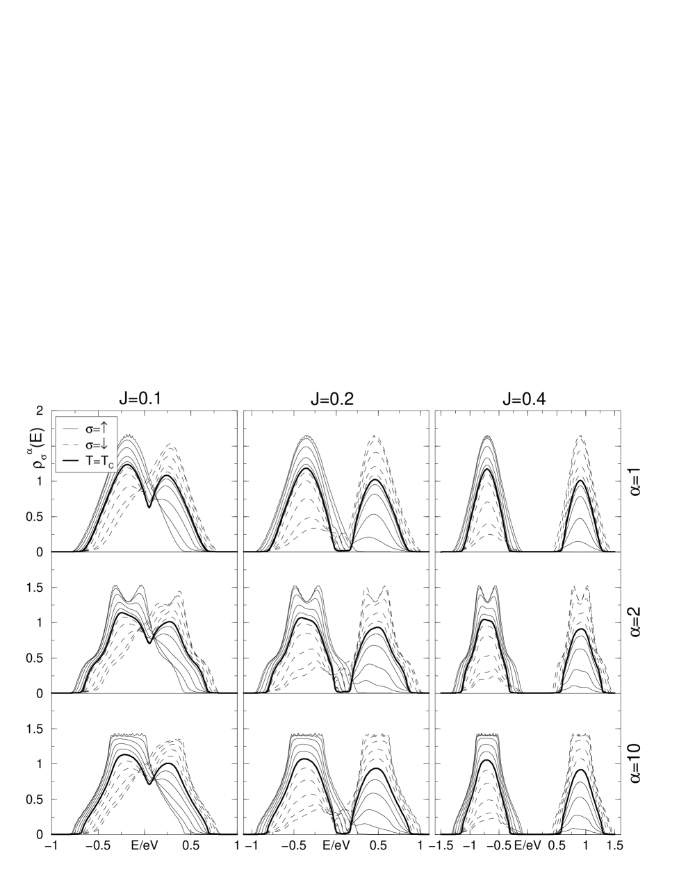
FIG. 8.: Local density of states, $\rho_{\sigma}^{\alpha}(E)$, of the first ($\alpha=1,20$), second ($\alpha=2,19$), and center ($\alpha=10,11$) layer of a 20-layer s.c.-(100) film for different s-f interactions $J$ and different temperatures $T/T_{C}=0,0.4,0.7,0.9,0.98,1$. The curves for $T=0$ are furthest away from the paramagnetic solution, $T=T_{C}$ (fat line).

In the case of ferromagnetic saturation there is no restriction for the propagation of the spin-$\uparrow$ electrons since spin-flip processes are impossible. With increasing temperature there is an increasing deviation of the local moments resulting in the possible magnon absorption by the spin-$\uparrow$ electron and subsequent changing to the higher energetic polaron subband. Hence, the spin-$\uparrow$ electron, to propagate in its own subband needs to move further distances with increasing temperature resulting in a reduced effective hopping and in a decreased bandwidth.

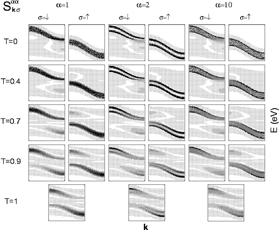
FIG. 9.: Spectral density, $S^{\alpha\alpha}_{{\bf k}\sigma}$, as a function of wavevector ${\bf k}$ from $\Gamma=(0,0)$ to ${\rm M}=(\pi,\pi)$ (horizontal axes) and energy $E$ from -1eV to 1eV (vertical axes) of the first ($\alpha=1,20$), second ($\alpha=2,19$), and center ($\alpha=10,11$) layer of a 20-layer s.c.-(100) film for $J=0.2$eV and different temperatures (in units of $T_{C}$).

In addition to the discussed temperature effects, Figs. 6 and 7 exhibit a typical two-peak structure which is caused by the coupling of the two layers. This two-peak structure is replaced in the case of a film consisting of $n$ equivalent layers by an $n$-peak structure. Generally, the spectra of the discussed local-moment films are characterised by an interplay between correlation ($J$), temperature effects, and geometry of the film. Figs. 8 and 9 display results for the local density of states and the layer-dependent spectral density of a 20-layer s.c.-(100)-film. Additionally to the dependence on the s-f exchange interaction and the temperature dependence we notice that the spectral density and the density of states show a typical layer-dependence due to the broken translational symmetry at the surfaces of the film [29]. For the centre layers ($\alpha=10,11$) of the 20-layer-film we see from Fig. 8 that the local density of states of the spin-$\uparrow$ electron at $T=0$ has already become pretty similar to the well-known tight-binding density of states of the three-dimensional s.c. lattice whereas the density of states of the surface layers ($\alpha=1,20$) exhibits the characteristic semi-elliptic profile.

IV Summary

We have investigated the electronic quasiparticle bandstructure of a ferromagnetic semiconductor film. A single test electron (s-band) is coupled by an intra-atomic s-f inter-band exchange to a system of localized 4f-moments. That may be regarded as a proper model description for Euo and EuS. Our approach uses a moment-conserving decoupling procedure for suitable defined Green functions. The fact that our theory evolves continuously from the exactly solvable limiting case of ferromagnetic saturation [29] gives it a certain trustworthiness.

The exchange coupling of the conduction electron to the local-moment system gives rise to a correlation induced splitting of the quasiparticle spectra. A polaron part may be interpreted as a repeated emission and reabsorption of magnons by the conduction electron resulting in a new quasiparticle, the magnetic polaron. A rather broad scattering peak is due to a simple magnon emission or absorption by the conduction electron. This pronounced splitting depends on the actual value of the exchange interaction $J$. For small values of $J$ only a renormalization of the one-electron energy occurs resulting in a deformation of the free Bloch dispersion. For higher values of $J$, the mentioned splitting of the spectra into polaron part and scattering part sets in.

We intend to apply the presented model to study the temperature dependent electronic structure of EuO and EuS films. Therefore the electronic part of the Hamiltonian (3) and the s-f exchange interaction (6) have to be modified to include the multiband aspect of real substances. This will be done by substituting the tight-binding bandstructure (85) by a realistic one taken from a bandstructure calculation.

Another highly interesting field which we want to use our theory for is the evaluation of the temperature dependence of surface states. In a previous paper we have calculated surface states for the special case of $T=0$ and $n=0$ by modifying the hopping in the vicinity of the surface [37]. The extension of these calculations to finite temperatures promises to give an understanding of recent experimental results concerning the temperature dependence of electronic states on surfaces of rare earths.

REFERENCES

• [1] Electronic address: roland.schiller@physik.hu-berlin.de
• [2] E. L. Nagaev, phys. stat. sol. (b) 65, 11 (1974).
• [3] W. Nolting, phys. stat. sol. (b) 96, 11 (1979).
• [4] P. Wachter, in Handbook of the Physics and Chemistry of Rare Earth, edited by J. K. A. Gschneidner and L. Eyring (North Holland, Amsterdam, 1979), Vol. 1, Chap. 19.
• [5] S. Legvold, in Ferromagnetic Materials, edited by E. P. Wohlfarth (North Holland, Amsterdam, 1980), Vol. 1, Chap. 3.
• [6] H. Tsunetsugu, M. Sigrist, and K. Ueda, Rev. Mod. Phys. 69, 809 (1997).
• [7] N. Furukawa, J. Phys. Soc. Japan 63, 3214 (1994).
• [8] E. Dagotto et al., Phys. Rev. B 58, 6414 (1998).
• [9] T. Wolfram and R. E. DeWames, Prog. Surf. Sci. 2, 233 (1972).
• [10] D. L. Mills, in Surface Excitations, edited by V. M. Agranovich and R. Loudon (North Holland, Amsterdam, 1984).
• [11] A. J. Freeman and C. L. Fu, in Magnetic Properties of Low Dimensional Systems, Vol. 14 of Springer Proceedings in Physics, edited by L. M. Falicov and J. L. Morán-López (Springer, Berlin, 1986), p. 16.
• [12] K. Binder, in Phase Transitions and Critical Phenomena, edited by C. Domb and J. L. Lebowitz (Academic Press, London, 1989), Vol. 8, Chap. 1.
• [13] R. Wu and A. J. Freeman, J. Magn. Magn. Mater. 99, 81 (1991).
• [14] P. A. Dowben, D. N. McIlroy, and D. Li, in Handbook of the Physics and Chemistry of Rare Earth, edited by J. K. A. Gschneidner and L. Eyring (Elsevier, Amsterdam, 1997), Vol. 24, Chap. 159.
• [15] T. Herrmann and W. Nolting, J. Phys.: Condens. Matter 11, 89 (1999).
• [16] D. Weller et al., Phys. Rev. Lett. 54, 1555 (1985).
• [17] C. Rau and S. Eichner, Phys. Rev. B 34, 6347 (1986).
• [18] C. Rau and M. Robert, Phys. Rev. Lett. 58, 2714 (1987).
• [19] H. Tang et al., Phys. Rev. Lett. 71, 444 (1993).
• [20] C. Rau, C. Jin, and M. Robert, J. Appl. Phys. 63, 3667 (1988).
• [21] C. Rau, C. Jin, and M. Robert, Phys. Lett. A 138, 334 (1989).
• [22] M. Donath, B. Gubanka, and F. Passek, Phys. Rev. Lett. 77, 5138 (1996).
• [23] A. V. Fedorov, K. Starke, and G. Kaindl, Phys. Rev. B 50, 2739 (1994).
• [24] E. Weschke et al., Phys. Rev. Lett. 77, 3415 (1996).
• [25] W. Nolting, T. Dambeck, and G. Borstel, Z. Phys. B 94, 409 (1994).
• [26] B. Kim et al., Phys. Rev. Lett. 68, 1931 (1992).
• [27] D. Li, J. Zhang, P. A. Dowben, and M. Onellion, Phys. Rev. B 45, 7272 (1992).
• [28] D. Li et al., J. Phys. C 4, 3929 (1992).
• [29] R. Schiller, W. Müller, and W. Nolting, J. Magn. Magn. Mater. 169, 39 (1997).
• [30] W. Nolting, S. M. Jaya, and S. Rex, Phys. Rev. B 54, 14455 (1996).
• [31] W. Nolting, S. Rex, and S. M. Jaya, J. Phys.: Condens. Matter 9, 1301 (1997).
• [32] S. R. Allan and D. M. Edwards, J. Phys. C 15, 2151 (1982).
• [33] W. Nolting and U. Dubil, phys. stat. sol. (b) 130, 561 (1985).
• [34] N. M. Mermin and H. Wagner, Phys. Rev. Lett. 17, 1133 (1966).
• [35] M. E. Lines, Phys. Rev. 156, 534 (1967).
• [36] R. Schiller and W. Nolting, Solid State Commun. 110, 121 (1999).
• [37] R. Schiller, W. Müller, and W. Nolting, Eur. Phys. J. B 2, 249 (1998).