Topological universality of level dynamics in quasi-one-dimensional
disordered conductors

Abstract

Nonperturbative, in inverse Thouless conductance $g^{-1}$, corrections to distributions of level velocities and level curvatures in quasi-one-dimensional disordered conductors with a topology of a ring subject to a constant vector potential are studied within the framework of the instanton approximation of nonlinear $\sigma$-model. It is demonstrated that a global character of the perturbation reveals the universal features of the level dynamics. The universality shows up in the form of weak topological oscillations of the magnitude $\sim e^{-g}$ covering the main bodies of the densities of level velocities and level curvatures. The period of discovered universal oscillations does not depend on microscopic parameters of conductor, and is only determined by the global symmetries of the Hamiltonian before and after the perturbation was applied. We predict the period of topological oscillations to be $4/\pi^{2}$ for the distribution function of level curvatures in orthogonal symmetry class, and $\sqrt{3}/\pi$ for the distribution of level velocities in unitary and symplectic symmetry classes.

I Introduction

Parametric level statistics describes the response of the spectrum $\{E_{n}\}$ of complex chaotic systems to an external perturbation, being a measure of the sensitivity of the individual energy level to a change of some external parameter $x$. The part of the parameter $x$ can be played by either the external electric or magnetic field, or the ‘strength’ of a background potential. It may be any other relevant parameter of the Hamiltonian.

In the series of papers [1, 2, 3], it was shown that a system whose spectrum follows closely the universal fluctuations predicted by the Wigner–Dyson random matrix theory [4] (RMT) should also exhibit a universal parametric behavior. This conclusion was reached by analyzing the correlations of the single electron level densities in a disordered metallic sample with the topology of a ring pierced by an Aharonov–Bohm magnetic flux $\varphi$. In this particular problem, the parametric correlations take a universal form involving the rescaled parameter $X^{2}\propto g\varphi^{2}$, with the dimensionless conductance $g=E_{c}/\Delta$, the ratio of the Thouless energy and the mean level spacing. Numerical simulations [2] have supported the point that the universal character of parametric level statistics extends to a wider class of chaotic systems without disorder (chaotic billiards) whose Hamiltonian depends on some external parameter $x$. In such systems, the spectral fluctuations taken at different values of $x$ become system-independent after the rescaling, $x\mapsto X$, which involves solely the ‘generalized’ dimensionless conductance $g\propto\Delta^{-2}\left\langle[\partial E_{n}(x)/\partial x]_{x=0}^{2}\right\rangle$. [Here, the angular brackets $\left\langle...\right\rangle$ stand for disorder averaging.] Further investigations [5, 6, 7] have established the universality of other parametric statistics such as the distribution functions $P_{v}(V)=\Delta\langle\sum_{n}\delta(V-V_{n})\delta(E-E_{n}(0))\rangle$ and $P_{c}(K)=\Delta\langle\sum_{n}\delta(K-K_{n})\delta(E-E_{n}(0))\rangle$ of the level velocities $V_{n}=\Delta^{-1}[\partial E_{n}(x)/\partial x]_{x=0}$ and the level curvatures $K_{n}=\Delta^{-1}[\partial^{2}E_{n}(x)/\partial x^{2}]_{x=0}$. These two measures of level dynamics turn out to be universal after the rescaling $V={\tilde{V}}\langle V_{n}^{2}\rangle^{1/2}$ and $K={\tilde{K}}\langle|K_{n}|\rangle$. Both distributions [8]

$$P_{v}(V)\propto\left\{\begin{array}[]{cc}\delta({\tilde{V}}),&\beta=1,\\ \exp\{-{\tilde{V}}^{2}/2\},&\beta=2,4,\end{array}\right.$$ (4)

and

$$P_{c}(K)\propto(1+{\tilde{K}}^{2})^{-1-\beta/2}$$ (5)

appear to depend only on the Dyson index [4] $\beta=1,2$ and $4$. In turn, the averages $\langle V_{n}^{2}\rangle$ and $\langle|K_{n}|\rangle$ are deeply connected, via the Edwards–Thouless relation [9], to the average system conductance if the parameter $x$ represents the Aharonov–Bohm flux. The latter circumstance makes it possible to use these rather abstract measures of level dynamics for distinguishing between the extended and the localized phases in disordered systems.

The above universality (that emerges after appropriate rescaling) implies that the resulting parametric correlations do not depend on details of the system and the perturbation. Instead, they are only determined by the fundamental (orthogonal, unitary or symplectic) symmetries of the system before and after it was perturbed. For disordered conductors, this universal regime is observed in the limit [10] of the infinite dimensionless conductance, $g=E_{c}/\Delta\rightarrow\infty$. In quantum chaotic systems, the same criterion [11] applies provided one identifies the Thouless energy with the first nonzero mode $\gamma_{1}$ in the spectrum of the Perron–Frobenius operator of the corresponding classical system. It should be stressed that the extended, structureless electron eigenfunctions which do not correlate with the fluctuations of the electron energy levels are the underlying physical reasons of the universality phenomenon.

One-dimensional conductors in the strongly localized regime constitute another extreme situation, in which the universality of parametric statistics is broken completely. Recent studies [12, 13] have shown that, in the regime of strong localization, the distribution function of level curvatures has nothing in common with the universal law Eq. (5). Instead, it roughly follows the log-normal law which explicitly contains such system-dependent parameters as the circumference $L$ of a one-dimensional ring and the electron mean free path $l$ (which is of order of the localization length $\xi$ for a one-channel conductor).

Disordered conductors with large but finite values of $g$, which are in between of the two extreme situations described above, offer a fertile field for tracing the mechanism of breaking the parametric universality. While, in this case, the electron wave functions are still extended, they do have a pronounced internal structure (showing up in their long-range correlations [14, 15]) that cannot already be neglected. Finite–$g$ corrections to parametric level statistics beyond the Wigner–Dyson RMT have been a focus of a number of studies [16, 17, 18]. All of them have emphasized a nonuniversal character of the level dynamics manifesting itself already in the form of the perturbative corrections [17] to the level curvature distribution which becomes sensitive to both the spatial dimensionality $d$ of the disordered conductor and the origin of the external perturbation. The latter determines the sign of the correction which depends on the presence or absence of the global gauge invariance (that is, on the topological origin of the perturbation) and is different for the $T$–breaking perturbations in the form of random magnetic fluxes that act locally and for the $T$–breaking perturbations represented by a constant vector potential (that is equivalent to a global phase twist in the boundary conditions). Nonanalyticity [19] of the level curvature distribution in the latter case in the low-dimensional conductors ($d=1,2$) was also addressed.

In the present paper we further examine the level dynamics in quasi-one-dimensional disordered conductors in the presence of the Aharonov–Bohm magnetic flux to demonstrate that, for finite conductance $g$, a new kind of topological universality emerges, for which the existence of the global gauge invariance is crucial. This is a nonperturbative in $g^{-1}$ effect. To be precise, we argue that the ring topology and the global character of the perturbation are responsible for appearance of the weak oscillations covering the main bodies, Eqs. (4) and (5), of the distributions of the level velocities and the level curvatures. While the magnitude of the oscillations is system dependent (being of order of $\sim e^{-g}$), their period appears to be independent of microscopic parameters of the system and the perturbation: It is entirely determined by the global symmetries – orthogonal, unitary or symplectic – of the system before and after the perturbation was applied, and is different for level velocities and level curvatures. We also stress that, contrary to the Wigner–Dyson universality [Eqs. (4) and (5)], that arises after rescaling $V\mapsto{\tilde{V}}$ and $K\mapsto{\tilde{K}}$, no rescaling is needed to establish the universality of topological oscillations: Their period is universal and parameter independent in genuine variables $V$ and $K$. In the absence of the global gauge invariance, the above universality does not show up at all.

To appreciate the difference between the local and the global perturbations on the formal level, it is instructive to appeal to the random matrix formulation of the problem, replacing the microscopic Hamiltonian by banded random matrices which are known [20] to describe (in a certain thermodynamic limit) the physics of disordered quasi-one-dimensional conductors. For definiteness, the orthogonal symmetry is supposed to be respected in the unperturbed conductor, while the perturbation is assumed to drive the system symmetry toward the unitary one.

(i) For the local perturbation of the strength $x$, the perturbed quasi-one-dimensional disordered system with $N$ sites can be modeled by the $N\times N$ parametric random matrix of the Pandey–Mehta type [21]

$$H^{\rm local}(x)=H^{R}+ixH^{A},$$ (6)

where $H^{R}$ and $H^{A}$ are $N\times N$ real symmetric and real antisymmetric, statistically independent banded random matrices, respectively. Notice that such a decomposition imposes no constraints for the real eigenvalues of the matrix $H^{\rm local}(x)$ as functions of the variable $x$.

(ii) This contrasts the case of the global perturbation applied to quasi-one-dimensional conductors with a ring topology which should explicitly be incorporated [22] to both unperturbed and perturbed matrix Hamiltonians. An unperturbed (real symmetric) matrix $H(0)$ must account for a periodic electron motion along a discrete ring of $N$ sites (see Fig. 1).

FIG. 1.: A discrete ring of $N$ sites pierced by a (dimensionless) Aharonov–Bohm flux $\varphi$. Connected geometry of a ring permits the electron hopping from the $N$-th site to $b$ adjacent sites to the left and $b$ sites to the right.

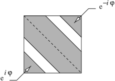
FIG. 2.: Schematic representation of the structure of the periodic banded matrix that contains three (shaded) regions with nonvanishing entries: The band of the width $2b$ along the main diagonal, the upper right and the lower left corners (both of the width $b$). In the presence of the Aharonov–Bohm flux, the corner entries are multiplied by the phase factors $e^{\pm i\varphi}$, Eq. (8).

If the particle located at some site may reach only $b$ neighbors to the right and $b$ neighbors to the left ($b<[N/2]$), it is easy to see that the unperturbed ‘periodic’ $N\times N$ matrix $H(0)$ will contain three regions with nonvanishing entries: a band $|\mu-\nu|\leq b$ along the main diagonal, and the upper right and the lower left corners, $|\mu-\nu|\geq N-b$ (see Fig. 2).

Let us now apply a small static magnetic flux $\Phi=(\varphi/2\pi)\Phi_{0}$, $\Phi_{0}=hc/e$ being the flux quantum. Each time the electron hops from the site $\mu$ to the site $\mu+1$, it ascribes the phase $\varphi/N$. As a result, the transition amplitude between the sites $\mu$ and $\nu$ gets modified by the phase factor $e^{i\theta_{\mu\nu}}$, $H_{\mu\nu}\mapsto H_{\mu\nu}e^{i\theta_{\mu\nu}}$, with

$$\theta_{\mu\nu}=\left\{\begin{array}[]{cc}[(\nu-\mu)/N]\varphi&\text{if }|\mu-\nu|\leq b,\\ {\rm sgn}(\mu-\nu)[1-|\nu-\mu|/N]\varphi&\text{if }|\mu-\nu|\geq N-b.\end{array}\right.$$ (7)

Passing on to the basis, in which the eigenvectors of the perturbed matrix are transformed as $\psi_{k}\mapsto\psi_{k}e^{i(k/N)\varphi}$, we arrive at the perturbed periodic matrix of the form

$$H_{\mu\nu}^{\rm global}(\varphi)=\left\{\begin{array}[]{cc}H_{\mu\nu}(0)&\text{if }|\mu-\nu|\leq b,\\ H_{\mu\nu}(0)e^{-i\varphi}&\text{if }\nu-\mu\geq N-b,\\ H_{\mu\nu}(0)e^{i\varphi}&\text{if }\mu-\nu\geq N-b.\end{array}\right.$$ (8)

The perturbed periodic matrix $H^{\rm global}$ obtained in this way possesses a manifestly different structure as compared to the structure of $H^{\rm local}$, hereby reflecting the presence of the global gauge invariance in the former case.

The structure of Eq. (8) dictates the $2\pi$–periodicity of the eigenvalues $E_{n}(\varphi)$ of $H^{\rm global}(\varphi)$,

$$E_{n}(\varphi+2\pi)=E_{n}(\varphi).$$ (9)

Equation (9) suggests the Fourier analysis to be an appropriate language for description of level dynamics in the case of the global perturbation:

$$E_{n}(\varphi)=\Delta\sum_{m=0}^{\infty}a_{m}^{(n)}\cos(m\varphi).$$ (10)

As a matter of fact, Eq. (10) allows one to relate the problem of evaluating the Fourier transform $\tilde{P}_{c}(\lambda)=\int dK\exp\{-iK\lambda\}P_{c}(K)$ of the curvature distribution function to an effective statistical mechanical problem. To see this, we notice that the level curvature $K_{n}$ can be expressed in terms of the amplitudes $a_{m}^{(n)}$ as

$$K_{n}=\frac{1}{\Delta}\left.\frac{\partial^{2}E_{n}}{\partial\varphi^{2}}\right|_{\varphi=0}=-\sum_{m=0}^{\infty}m^{2}a_{m}^{(n)},$$ (11)

so that the Fourier transform $\tilde{P}_{c}(\lambda)$ of the curvature distribution function is

$$\tilde{P}_{c}(\lambda)=\Delta\left\langle\sum_{n}\exp\left\{i\lambda\sum_{m=0}^{\infty}m^{2}a_{m}^{(n)}\right\}\delta(E-E_{n}(0))\right\rangle.$$ (12)

Introducing the joint probability distribution function for the amplitudes $a_{m}^{(n)}$ in the form

$${\cal P}_{g}(\{a_{m}\})=\Delta\left\langle\sum_{n}\delta(E-E_{n}(0))\prod_{m=0}^{\infty}\delta(a_{m}-a_{m}^{(n)})\right\rangle,$$ (13)

we conclude that the free energy $\tilde{F}_{c}(\lambda)=-\ln\tilde{P}_{c}(\lambda)$ of the effective statistical mechanical model equals

$$\tilde{F}_{c}(\lambda) = -\lim_{M\rightarrow\infty}\ln\int\prod_{m=0}^{M}da_{m}{\cal P}_{g}(\{a_{m}\})$$ (14)

$$\times \exp\left\{i\lambda\sum_{m=0}^{M}m^{2}a_{m}\right\}.$$ (15)

Here, ${\cal P}_{g}(\{a_{m}\})$ describes the interaction of fictitious ‘particles’ $a_{m}$ subject to external ‘field’ $i\lambda$. [Similar representation can be obtained for the distribution function of the level velocities $V_{n}$ for $\beta=2,4$. In this case, $\cos(m\varphi)$ is to be replaced by $\sin(m\varphi)$ in the Fourier expansion Eq. (10).] It is important to emphasize that no such mapping to an effective statistical mechanical problem is available for the case of the local perturbation, Eq. (6).

In the rest of the paper, we argue, by using the instanton approximation [23, 19] of nonlinear $\sigma$-model, that in the limit $g\gg 1$ the effective statistical mechanical model Eq. (14) exhibits a second-order phase transition as the external field $i\lambda$ varies, with the free energy $\tilde{F}_{c}(\lambda)$ displaying a discontinuity of its second derivative at the ‘critical’ point determined by the value of the critical parameter $\lambda_{c}=\pi^{3}/2$. It turns out, that the value of the critical field $i\lambda_{c}$ is universal: It does not depend on microscopic parameters of the problem but is entirely determined by the global character of the perturbation, Eq. (8), that breaks the orthogonal symmetry toward the unitary one. This finding, being translated to the space of genuine curvature variable $K$, implies appearance of the universal oscillations with the universal period $\delta K=2\pi/\lambda_{c}=4/\pi^{2}$ and the system-dependent amplitude $\sim e^{-g}$ on the main body Eq. (5) of the level curvature distribution. Similar analysis of the distribution functions of the level velocities (at $\beta=2$ and $4$) reveals the existence of the second-order phase transition in associated effective statistical mechanical problem as well. In the latter problem, the value of the critical external field $i\lambda_{c}$ is also found to be universal though different: $\lambda_{c}=2\pi^{2}/\sqrt{3}$. As a result, the main body Eq. (4) of the distribution function of the level velocities gets dressed by the weak oscillations of the same magnitude ($\sim e^{-g}$) with the universal period $\delta V=2\pi/\lambda_{c}=\sqrt{3}/\pi$. We stress that the above universality has a clear topological origin: A global character of the perturbation (constant vector potential) and a ring geometry of a quasi-one-dimensional conductor are necessary conditions for its existence.

The paper is organized as follows. Section II is devoted to a nonperturbative analysis of the level curvature distribution function associated with the global $T$–breaking perturbation over the orthogonal ensemble. The distribution of the level velocities in ensemble with the unitary symmetry is analyzed in Section III. In Section IV a relationship between the ring geometry of a conductor, the boundary conditions in associated nonlinear $\sigma$-model (in its quasi-one-dimensional and ergodic limits) and the discovered topological oscillations is discussed. Section V contains conclusions. The details concerning the distribution function of the level velocities in the case of symplectic symmetry are collected in Appendix.

II Distribution of level curvatures at $\beta=1$

Let us consider the electron of mass $m$ moving in a disordered conductor with a topology of a quasi-one-dimensional ring of the circumference $L$. In the presence of the magnetic flux $\Phi$ that pierces the ring, the one-particle Hamiltonian takes the form

$${\hat{H}}=\frac{\hbar^{2}}{2m}\left(i{\bf\nabla}_{\bf r}+\frac{\varphi}{L}{\bf e}_{\theta}\right)^{2}+V({\bf r}),$$ (16)

where $\varphi=2\pi\Phi/\Phi_{0}$, $\Phi_{0}=hc/e$ is the flux quantum, and ${\bf e}_{\theta}$ is the unit vector along the azimuthal direction. The potential $V({\bf r})$ describes the effect of disorder and is supposed to be the $\delta$-correlated random Gaussian process with $\langle V({\bf r})V({\bf r^{\prime}})\rangle=(\hbar/2\pi\nu\tau)\delta({\bf r}-{\bf r^{\prime}})$. Here, $\tau$ is the mean time between collisions and $\nu$ is the density of states. The (dimensionless) magnetic flux $\varphi$ in the Hamiltonian breaks the time-reversal invariance which has been respected in the absence of the perturbation.

In what follows we are interested in the distribution function $P_{c}(K)=\Delta\langle\sum_{n}\delta(K-K_{n})\delta(E-E_{n}(0))\rangle$ of the level curvatures

$$K_{n}=\frac{2}{\Delta}\lim_{\varphi\rightarrow 0}\frac{E_{n}(\varphi)-E_{n}(0)}{\varphi^{2}}$$ (17)

fluctuating, for a given level, over the ensemble of disorder realizations. These fluctuations are due to fluctuations of both the single electron eigenfunctions and the electron eigenlevels in an unperturbed system. [Here, $\Delta$ is the mean level spacing.] Distribution function of level curvatures can be expressed through the parametric two-level correlation function $R(\omega,\varphi)=\Delta^{2}\langle\nu(E+\omega,\varphi)\nu(E,0)\rangle$ by means of the limiting procedure [17]

$$P_{c}(K)=\lim_{\varphi\rightarrow 0}\frac{\varphi^{2}}{2}R\left(\omega=\frac{K\varphi^{2}\Delta}{2},\varphi\right),$$ (18)

similar to the one suggested in Ref. [24] for the distribution of the level velocities. The relation Eq. (18) is based on the fact that the level velocity vanishes identically in ensembles with the weakly broken orthogonal symmetry, Eq. (4).

The parametric two-level correlation function $R(\omega,\varphi)$, and hence the distribution function $P_{c}(K)$ of the level curvatures, can be represented in the form of the functional integral over the $8\times 8$ supermatrix field $Q$ by using the Efetov’s nonlinear $\sigma$-model [10]. The latter statistics is given by [6, 17]

$$P_{c}(K)=\lim_{\varphi\rightarrow 0}\varphi^{2}{\rm Re}\int_{Q^{2}(x)=\openone_{8}}{\cal D}Qp_{c}[Q]\exp\{-F[Q;K,\varphi]\}.$$ (19)

Here, $p_{c}[Q]$ is some preexponent irrelevant for our further consideration that holds with the exponential accuracy. The free energy functional $F[Q;K,\varphi]$ reads:

$$F[Q;K,\varphi] = \frac{\pi g}{8}\int dx{\rm Str}\left(\partial_{x}Q-i\varphi\left[{\hat{\tau}},Q\right]\right)^{2}$$ (20)

$$+ \frac{i\pi K\varphi^{2}}{8}\int dx{\rm Str}\left(\Lambda Q\right).$$ (21)

In the above formulas, $x=r/L\in(-1/2,+1/2)$ is the dimensionless coordinate measured along the ring, $g=\hbar D/L^{2}\Delta$ is the dimensionless conductance, $g\gg 1$.

For the ring topology the supermatrix field $Q(x)$ must obey the periodic boundary conditions. Its symmetry properties are specified in Ref. [10], so that $Q(x)$ spans the three subspaces: retarded–advanced (R-A), boson–fermion (B-F), and the subspace related to the time reversal (T-R). The supertrace, ${\rm Str}$, is defined as ${\rm Str}M={\rm Tr}M_{FF}-{\rm Tr}M_{BB}$. Other matrices entering Eq. (20) are

$${\hat{\tau}}=\frac{\openone_{8}+\Lambda}{2}{\hat{\tau}_{3}},$$ (22)

with

$${\hat{\tau}_{3}} = {\rm diag}\left(\sigma_{z},\sigma_{z},\sigma_{z},\sigma_{z}\right)_{\rm R-A},$$ (23)

$$\Lambda = {\rm diag}\left(\openone_{2},\openone_{2},-\openone_{2},-\openone_{2}\right)_{\rm R-A},$$ (24)

and

$$\sigma_{z}=\left(\begin{array}[]{cc}1&0\\ 0&-1\end{array}\right)$$ (27)

being the $z$-Pauli matrix in the T-R space. The matrix $\Lambda$ describes breaking the symmetry between the retarded and the advanced subspaces, while the matrix ${\hat{\tau}_{3}}$ breaks the time reversal symmetry.

Notice that the operator $\partial_{x}-i\varphi[{\hat{\tau}},...]$ in Eq. (20) implies the presence of the global gauge invariance due to the global character of the applied $T$–breaking perturbation represented by the Aharonov–Bohm flux $\varphi$. This operator gets destroyed if the perturbation has a local origin, that is the case of random magnetic fluxes or magnetic impurities. In this local case, the term linear in $\varphi$ is absent in Eq. (20).

It was realized in Refs. [19] that the level curvature $K$ enters the free energy functional Eq. (20) in the same way as does $\omega$ in the problem of the long-time current relaxation [23]. This observation suggests that the instanton approximation of nonlinear $\sigma$-model should be applicable to the evaluation of the Fourier transform, Eq. (12), of the level curvature distribution:

$${\tilde{P}}_{c}(\lambda) = \lim_{\varphi\rightarrow 0}\varphi^{2}{\rm Re}$$ (28)

$$\times \int dK\int_{Q^{2}(x)=\openone_{8}}{\cal D}Qp_{c}[Q]e^{-\left(F[Q;K,\varphi]+iK\lambda\right)}$$ (29)

$$\propto {\rm Re}\;e^{-(F[Q_{\rm ins};K_{\rm sp},0]+iK_{\rm sp}\lambda)}.$$ (30)

Equation (28) holds with the exponential accuracy, and is valid whenever the functional $F[Q_{\rm ins};K_{\rm sp},0]+iK_{\rm sp}\lambda$ is large enough. [Hereafter, we consider only positive values of $\lambda$ because of the evenness of $P_{c}(K)$.]

An important remark is appropriate here. In accordance with the results of Ref. [23] one can expect that at large enough $\lambda$ the space-independent configurations of $Q(x)$ are energetically unfavorable: There are essentially space-dependent, periodic superfields $Q_{\rm ins}(x)$ which minimize the functional in question. In contrast, at relatively small $\lambda$ we expect that the minimum of $F[Q;K,\varphi]+iK\lambda$ in the limit $\varphi\rightarrow 0$ is reached on spatially independent configurations of $Q(x)$. This formal argumentation suggests the existence of some ‘critical’ point $\lambda=\lambda_{c}$ at which a transition between the two solutions occurs. Below, this scenario will be confirmed by explicit calculations. It turns out that at the critical point the functional $F[Q_{\rm ins};K_{\rm sp},0]+iK_{\rm sp}\lambda$ and its first derivative with respect to $\lambda$ are continuous functions of $\lambda$, and only the second derivative exhibits a discontinuity with immediate implications for the distribution function $P_{c}(K)$ itself to be discussed later on.

Two observations are to be made before we proceed with the computation of ${\tilde{P}}_{c}(\lambda)$. First, we note that due to the limit $\varphi\rightarrow 0$ to be taken in Eq. (28) the only nonzero contribution to ${\tilde{P}}_{c}(\lambda)$ can arise from the entries in the noncompact boson–boson sector of the supermatrix $Q(x)$ because they are allowed to take arbitrary large values. Second, the integration over the Grassmann entries of $Q(x)$ modifies only the preexponent $p_{c}[Q]$ in Eq. (28) and, therefore, they do not contribute to ${\tilde{P}}_{c}(\lambda)=\exp\{-{\tilde{F}}_{c}(\lambda)\}$ if the latter is evaluated with the exponential accuracy, provided ${\tilde{F}}_{c}(\lambda)\gg 1$. For these two reasons, we may retain only the commuting entries in the noncompact sector of $Q(x)$ in Eq. (28). Hence, the supermatrix $Q$ may be thought of as a conventional $4\times 4$ matrix $Q_{B}(x)$.

Using the Efetov’s parameterization [10] for the orthogonal symmetry class, we obtain

$$Q_{B}\left(x\right)=U(x)\left(\begin{array}[]{cc}\cos{\hat{\theta}}_{B}&i\sin{\hat{\theta}}_{B}\\ -i\sin{\hat{\theta}}_{B}&-\cos{\hat{\theta}}_{B}\end{array}\right)_{{\rm R-A}}U^{-1}(x),$$ (31)

where

$$U(x)=\left(\begin{array}[]{cc}e^{i\phi\sigma_{z}}&0\\ 0&e^{i\chi\sigma_{z}}\end{array}\right)_{\rm R-A}$$ (34)

and

$$\cos{\hat{\theta}}_{B} = \cosh\theta_{1}\cosh\theta_{2}\openone_{2}+\sinh\theta_{1}\sinh\theta_{2}\sigma_{x},$$ (36)

$$\sin{\hat{\theta}}_{B} = i\sinh\theta_{1}\cosh\theta_{2}\openone_{2}+i\cosh\theta_{1}\sinh\theta_{2}\sigma_{x}.$$ (37)

Here,

$$\sigma_{x}=\left(\begin{array}[]{cc}0&1\\ 1&0\end{array}\right)$$ (40)

is the $x$-Pauli matrix in the T-R space; $z$-Pauli matrix was specified in Eq. (27).

In the equations above, $\phi,\chi\in(0,2\pi)$ and $\theta_{1},\theta_{2}\in(0,+\infty)$ are spatially dependent, periodic functions of the variable $x\in(-1/2,+1/2)$. Obviously, this periodicity reflects the ring topology of the disordered conductor in question. Substituting $Q_{B}(x)$ in the parameterization Eqs. (31) – (II) into Eq. (20), and varying the functional $F[Q;K,\varphi]+iK\lambda$ with respect to the functions $\theta_{1}(x)$, $\theta_{2}(x)$, $\phi(x)$ and $\chi(x)$ we find a set of four saddle-point equations which are satisfied by the choice $\theta_{1}(x)=\theta_{2}(x)=\theta(x)$ and $\phi(x)={\rm const}$. The functions $\theta(x)$ and $\chi(x)$ obey the following saddle-point equations:

$$\frac{d^{2}}{dx^{2}}[2\theta(x)]+\sinh[2\theta(x)]\left[\kappa\varphi^{2}-\left(\frac{d}{dx}\chi(x)-\varphi\right)^{2}\right]=0,$$ (41)

$$\frac{d}{dx}\left[\left(\frac{d}{dx}\chi(x)-\varphi\right)\sinh^{2}\theta(x)\right]=0,$$ (42)

where we have introduced $\kappa=iK_{\rm sp}/2g$. Also, variation over $K$ yields the first self-consistency equation

$$\varphi^{2}\int dx\cosh^{2}\theta(x)=2\lambda.$$ (43)

In terms of solutions to the above saddle-point equations, the functional ${\tilde{F}}_{c}(\lambda)=F[Q_{\rm ins};K_{\rm sp},0]+iK_{\rm sp}\lambda$ reads

  

$${\tilde{F}}_{c}(\lambda)=\lim_{\varphi\rightarrow 0}\left\{\pi g\int dx\left[\left(\frac{d\theta}{dx}\right)^{2}+\sinh^{2}\theta(x)\left(\frac{d\chi}{dx}-\varphi\right)^{2}-\kappa\varphi^{2}\cosh^{2}\theta(x)\right]+2g\kappa\lambda\right\}.$$ (44)

  

Notice that Eq. (44) is justified as long as ${\tilde{F}}_{c}(\lambda)\gg 1$.

In order to perform the limit $\varphi\rightarrow 0$, we introduce two new functions $v(x)=\chi(x)/\varphi$ and ${\tilde{\theta}}(x)=\theta(x)+\ln\varphi$ to reduce Eqs. (41) and (42) to

$$\frac{d^{2}{\tilde{\theta}}}{dx^{2}}+\frac{1}{4}e^{2{\tilde{\theta}}(x)}\left[\kappa-\left(\frac{dv}{dx}-1\right)^{2}\right]=0,$$ (45)

$$\frac{d}{dx}\left[\left(\frac{dv}{dx}-1\right)e^{2{\tilde{\theta}}(x)}\right]=0,$$ (46)

with ${\tilde{\theta}}(x)\in(-\infty,+\infty)$. The first self-consistency equation Eq. (43) takes the form

$$\int dxe^{2{\tilde{\theta}}(x)}=8\lambda,$$ (47)

and

$${\tilde{F}}_{c}(\lambda)=\pi g\int dx\left(d{\tilde{\theta}}/dx\right)^{2}+2g\kappa\lambda.$$ (48)

When deriving Eq. (48), we have taken into account Eq. (45), as well as the periodicity of ${\tilde{\theta}}^{\prime}(x)$.

Saddle-point equations Eqs. (45) and (46) correspond to the global $T$–breaking perturbation as is set by Eqs. (16) and (20). For the local perturbation, the linear in $\varphi$ term disappears from the functional Eq. (20) leading to the replacement of the terms $(dv/dx-1)^{2}$ and $dv/dx-1$ by the terms $(dv/dx)^{2}+1$ and $dv/dx$ in Eqs. (45) and (46), respectively. It can be shown [18] that the modified Eq. (46) and the periodicity of $v(x)$ result in the condition $dv/dx=0$ which, in turn, leaves the only possibility to satisfy the modified Eq. (45) by a spatially homogeneous configuration of ${\tilde{\theta}}(x)$ at $\kappa=1$. This corresponds to the universal Wigner–Dyson regime (see also the discussion (i) after Eq. (58)).

Now we are back to Eqs. (45) – (48) which can be brought to a more convenient form. Resolving Eq. (46), and making use of the periodicity of $v(x)$ we obtain

$$\int dxe^{-2{\tilde{\theta}}(x)}={\cal N}.$$ (49)

This is the second self-consistency equation. Further, introducing the new notations

$$w(x) = {\tilde{\theta}}(x)-\xi,$$ (51)

$$e^{-\xi} = {\cal N}\sqrt{\kappa},$$ (52)

we rewrite the only remained saddle-point equation Eq. (45) as

$$\frac{d^{2}w}{dx^{2}}+\sigma^{2}\sinh w(x)=0,$$ (54)

$$\sigma^{2}=\sqrt{\kappa}/{\cal N}.$$ (55)

It should be supplemented by the two self-consistency equations which we combine to

$$\int dxe^{\pm w(x)}=\frac{1}{\sqrt{\kappa}}=\frac{8\lambda{\cal N}\sqrt{\kappa}}{\pi}.$$ (56)

Here, the periodicity of $w^{\prime}(x)$ has explicitly been taken into account. Also,

$${\tilde{F}}_{c}(\lambda)=\frac{\pi g}{4}\int dx\left(\frac{dw}{dx}\right)^{2}+2g\kappa\lambda.$$ (57)

Equation (II) is an equation of motion of a classical particle with a unit mass in the potential

$$U(w)=\sigma^{2}[\cosh w-1],$$ (58)

$w$ and $x$ playing the role of coordinate and time, respectively. Due to a ring topology of our problem, we are interested in those solutions to Eq. (II) that describe the finite motion of the particle with the period $T=1$. There are two kinds of solutions available.

(i) The first solution is a trivial one, $w(x)=0$. In this case, one concludes from Eq. (56) that the saddle-point value of $K_{\rm sp}$ is given by $\kappa=1$. Equation (57) then tells us that ${\tilde{F}}_{c}(\lambda)\equiv{\tilde{F}}_{c}^{{\rm WD}}(\lambda)=2g\lambda$ for arbitrary $\lambda\geq 0$. One can verify, by making use [25] of Eq. (5) of Introduction for $\beta=1$, that this trivial solution appears to describe (with the exponential accuracy) the distribution of the level curvatures in the universal, Wigner–Dyson regime.

(ii) There is, however, the second solution which is spatially inhomogeneous. The important point here is that the finite motion in the potential $U(w)$ cannot occur with an arbitrary period. It is bounded from above, $T({\cal E})\leq T_{\rm max}=2\pi/\sigma$, with

$$T({\cal E})=\sqrt{2}\int_{w_{-}({\cal E})}^{w_{+}({\cal E})}\frac{dw}{\sqrt{{\cal E}-U(w)}}=\frac{4{\bf K}(k)}{\sigma}(1-k^{2})^{1/4}.$$ (59)

Here, $w_{\pm}$ are the turning points of the finite motion, $U(w_{\pm})={\cal E}$, and ${\cal E}$ is the integral of motion

$${\cal E}=\frac{1}{2}\left(\frac{dw}{dx}\right)^{2}+\sigma^{2}[\cosh w-1].$$ (60)

The parameter $k\in(0,1)$ is defined by

$$k^{2}=\frac{2\sqrt{\left(1+{\cal E}/\sigma^{2}\right)^{2}-1}}{\left(1+{\cal E}/\sigma^{2}\right)+\sqrt{\left(1+{\cal E}/\sigma^{2}\right)^{2}-1}},$$ (61)

${\bf K}(k)={\bf F}(\pi/2,k)$, with

$${\bf F}(\psi,k)=\int_{0}^{\psi}\frac{d\alpha}{\sqrt{1-k^{2}\sin^{2}\alpha}}$$ (62)

being the elliptic integral of the first kind [26].

The maximal period $T_{\rm max}$ corresponds to the almost harmonic particle oscillations in a vicinity of the minimum $w=0$ of the potential $U(w)$. Alternatively, for a given period $T=1$ (which we are interested in), the nontrivial period–$1$ solution exists only for $\sigma\leq\sigma_{c}=2\pi$. It is given by

$$x-\frac{1}{2} = -\frac{{\bf F}(\psi(x),k)}{2{\bf K}(k)},$$ (64)

$$\psi(x) = \arcsin\left(\frac{1}{k}\sqrt{1-\sqrt{1-k^{2}}e^{w(x)}}\;\right).$$ (65)

Equation (II) makes it possible to complete our computational program. To this end, we substitute Eq. (II) into Eq. (56) to obtain

$$\int dxe^{\pm w(x)}=\frac{{\bf E}(k)}{\sqrt{1-k^{2}}{\bf K}(k)}.$$ (66)

Here, ${\bf E}(k)={\bf E}(\pi/2,k)$ is the elliptic integral of the second kind [26]

$${\bf E}(\psi,k)=\int_{0}^{\psi}d\alpha\sqrt{1-k^{2}\sin^{2}\alpha}.$$ (67)

Further, we insert Eq. (II) into Eq. (57) and take into account Eqs. (60), (66), (56), (55) as well as the identity

$$\sigma=4{\bf K}(k)(1-k^{2})^{1/4}$$ (68)

following from Eq. (59) taken at $T=1$, to derive after some algebra the instanton solution ${\tilde{F}}_{c}(\lambda)\equiv{\tilde{F}}_{c}^{\rm ins}(\lambda)$ in the form

$${\tilde{F}}_{c}^{{\rm ins}}(\lambda)=4\pi g{\bf K}(k)\left[(2-k^{2}){\bf K}(k)-{\bf E}(k)\right].$$ (69)

FIG. 3.: The function ${\tilde{F}}_{c}(\lambda)$ given by Eq. (74). The dashed line depicts the Wigner–Dyson solution extended to the region $\lambda>\lambda_{c}$. A jump of the ‘heat capacity’ $C_{c}(\lambda)$ at the critical point $\lambda=\lambda_{c}$ is shown in the inset.

It remains to find the relationship between the initial parameter $\lambda$ of the Fourier space in the l.h.s. of Eq. (69) and the auxiliary parameter $k$. This is done by combining Eqs. (55), (56), (66) and (68) with the result

$$\lambda(k)=\frac{2\pi}{1-k^{2}}\frac{{\bf E}^{3}(k)}{{\bf K}(k)}.$$ (70)

Let us analyze Eqs. (69) and (70) which are manifestly different from ${\tilde{F}}_{c}^{{\rm WD}}(\lambda)=2g\lambda$ with $\lambda\geq 0$. It was already argued that the nontrivial solution Eq. (II) occurs at $\sigma\leq\sigma_{c}=2\pi$. As is seen from Eqs. (68) and (70), this domain maps to $0\leq k\leq 1$ with $k_{c}=0$, and/or to $\lambda\geq\lambda(0)=\lambda_{c}$, with

$$\lambda_{c}=\frac{\pi^{3}}{2}.$$ (71)

Exactly at the point $\lambda=\lambda_{c}$ one observes that ${\tilde{F}}_{c}^{{\rm ins}}(\lambda_{c})\equiv{\tilde{F}}_{c}^{{\rm WD}}(\lambda_{c})$, while at $\lambda\geq\lambda_{c}$ the inequality ${\tilde{F}}_{c}^{{\rm ins}}(\lambda)\leq{\tilde{F}}_{c}^{{\rm WD}}(\lambda)$ holds. [In particular, it follows from Eqs. (69) and (70) that [19] ${\tilde{F}}_{c}^{\rm ins}(\lambda)=\pi g\ln^{2}\lambda$ as $\lambda\gg 1$.] This means that for $\lambda\geq\lambda_{c}$ it is the spatially inhomogeneous, periodic solution Eq. (II) to the saddle-point equation Eq. (II) that minimizes the functional $F[Q;K,\varphi]+iK\lambda$ in Eq. (28) as $\varphi\rightarrow 0$. Therefore, we are forced to conclude that

$${\tilde{F}}_{c}(\lambda)=\left\{\begin{array}[]{cc}2g\lambda&\text{for }0\leq\lambda<\lambda_{c},\\ {\tilde{F}}_{c}^{\rm ins}(\lambda)&\text{for }\lambda\geq\lambda_{c}.\end{array}\right.$$ (74)

The result Eq. (74) supports the qualitative arguments given after Eq. (28).

A distinctive feature of Eq. (74), which holds as long as $g\gg 1$, is that the second derivative of ${\tilde{F}}_{c}(\lambda)$ with respect to $\lambda$ exhibits a discontinuity exactly at the critical point $\lambda=\lambda_{c}$, in whose vicinity $|\lambda-\lambda_{c}|\ll\lambda_{c}$ we derive

$$\frac{{\tilde{F}}_{c}(\lambda)}{g}=2\lambda-\frac{2\pi^{3}}{5}\Theta(\lambda-\lambda_{c})\left(1-\frac{\lambda}{\lambda_{c}}\right)^{2}.$$ (75)

One can define the ‘heat capacity’ $C_{c}(\lambda)=-d^{2}{\tilde{F}}_{c}/d\lambda^{2}$ which undergoes a jump at $\lambda=\lambda_{c}$: $C_{c}(\lambda)=0$ for $0\leq\lambda<\lambda_{c}$, and $C_{c}(\lambda)=16g/5\pi^{3}$ for $\lambda=\lambda_{c}+0$. This is the same discontinuity which is characteristic of the usual second-order phase transitions treated in the mean-field approximation, the factor $g$ playing the role of the ‘volume’. Equation (75) is an evidence to the second-order phase transition in the effective statistical mechanical model Eq. (14) proposed in the Introduction.

The above discontinuity (revealed in the Fourier space $\lambda$) has an important impact upon the distribution of the level curvatures. Being translated to the space of genuine curvature variable $K$, Eq. (75) implies appearance of the weak oscillations covering the main body of the distribution function of the level curvatures, with a system-dependent amplitude of order $\sim e^{-g}$ and the universal period

$$\delta K=\frac{2\pi}{\lambda_{c}}=\frac{4}{\pi^{2}}.$$ (76)

We stress that the value of $\delta K$ does not depend on microscopic parameters of the Hamiltonian Eq. (16). Its value is only determined by the ring topology of the disordered conductor as well as by the orthogonal symmetry of the problem weakly broken by the global external perturbation in the form of a constant vector potential.

We close this section by noticing that the above universal oscillations do not appear for the local perturbation. In that case, neither the statistical mechanical model Eq. (14) can be introduced, nor are the nontrivial periodic configurations of the $Q$-matrix available in associated nonlinear $\sigma$-model [18]. This signals of a topological origin of the discovered oscillations.

III Distribution of level velocities at $\beta=2$

In this section, we extend the previous analysis to study manifestations of the gauge invariance in the distribution function of the single electron level velocities in quasi-one-dimensional disordered ring where the time reversal symmetry has been broken from the very beginning so that the additionally applied small magnetic field respects the initial (unitary) symmetry of the problem. As is the case of the curvature distribution, the distribution $P_{v}(V)=\Delta\langle\sum_{n}\delta(V-V_{n})\delta(E-E_{n}(0))\rangle$ of the level velocities

$$V_{n}=\frac{1}{\Delta}\lim_{\varphi\rightarrow 0}\frac{E_{n}(\varphi)-E_{n}(0)}{\varphi}$$ (77)

can be expressed through the parametric two-level correlation function $R(\omega,\phi)$ by means of the limiting procedure

$$P_{v}(V)=\lim_{\varphi\rightarrow 0}\varphi R\left(\omega=V\varphi\Delta,\varphi\right),$$ (78)

as first proposed in Ref. [24].

We take the conventional route, and express the parametric two-level correlation function in terms of the nonlinear $\sigma$-model. The desired distribution of level velocities is

$$P_{v}(V)=\lim_{\varphi\rightarrow 0}\varphi{\rm Re}\int_{Q^{2}(x)=\openone_{8}}{\cal D}Qp_{v}[Q]\exp\left\{-F[Q;V,\varphi]\right\}.$$ (79)

Here, $p_{v}[Q]$ is some preexponent which is irrelevant for our calculations performed with the exponential accuracy. The free energy functional in Eq. (79) reads

$$F[Q;V,\varphi] = \frac{\pi g}{8}\int dx{\rm Str}\left(\partial_{x}Q-i\varphi[{\hat{\tau}},Q]\right)^{2}$$ (80)

$$+ \frac{i\pi V\varphi}{4}\int dx{\rm Str}(\Lambda Q).$$ (81)

Despite the similarity of Eq. (80) to Eq. (20), the symmetry properties [10] of the $8\times 8$ supermatrix field $Q$ are different in these two situations. [In particular, under assumption that the time reversal symmetry is completely destroyed, one has [2, 27] $[Q,{\hat{\tau}_{3}}]=0$.]

Evaluation of the Fourier transform of the distribution function of level velocities is the main goal of this section. In the instanton approximation used above one obtains (with the exponential accuracy)

$${\tilde{P}}_{v}(\lambda)=\int dVP_{v}(V)e^{-iV\lambda}\propto{\rm Re}\;e^{-(F[Q_{{\rm ins}};V_{\rm sp},0]+iV_{\rm sp}\lambda)},$$ (82)

where $\lambda$ is considered to be positive, $\lambda\geq 0$, owing to the evenness of $P_{v}(V)$. Let us proceed as follows. Due to the limit $\varphi\rightarrow 0$ to be implemented, we have to retain only noncompact degrees of freedom in the supermatrix $Q$ which are given by its boson–boson sector. Simultaneously, we omit the Grassmann entries, as discussed in the previous section. As a result, we replace $8\times 8$ supermatrix $Q$ by conventional $4\times 4$ matrix $Q_{B}$ in the parameterization of Eqs. (31) and (34), in which

$$\cos{\hat{\theta}}_{B} = \cosh\theta_{1}\openone_{2},$$ (84)

$$\sin{\hat{\theta}}_{B} = i\sinh\theta_{1}\openone_{2}.$$ (85)

Here, $\phi,\chi\in(0,2\pi)$ and $\theta_{1}\in(0,+\infty)$ are spatially dependent, periodic functions of the variable $x\in(-1/2,+1/2)$. Substituting $Q_{B}(x)$ into Eq. (80), and varying the functional $F[Q;V,\varphi]+iV\lambda$ with respect to the functions $\theta_{1}(x)=\theta(x)$, $\phi(x)$ and $\chi(x)$, we find the following set of the saddle-point equations that determine the instanton configuration $Q_{\rm ins}$:

$$\frac{d^{2}\theta}{dx^{2}}+\sinh\theta(x)\left[\frac{\kappa}{2}\varphi-\left(\frac{d}{dx}\chi(x)-\varphi\right)^{2}\cosh\theta(x)\right]=0,$$ (86)

$$\frac{d}{dx}\left[\left(\frac{d}{dx}\chi(x)-\varphi\right)\sinh^{2}\theta(x)\right]=0.$$ (87)

Here, we have introduced $\kappa=2iV_{\rm sp}/g$. Also, one has $\phi(x)={\rm const}$.

Variation over $V$ yields the first self-consistency equation

$$\pi\varphi\int dx\cosh\theta(x)=\lambda.$$ (88)

In terms of the above functions, the functional ${\tilde{F}}_{v}(\lambda)=F[Q_{\rm ins};V_{\rm sp},0]+iV_{\rm sp}\lambda$ takes the form

  

$${\tilde{F}}_{v}(\lambda)=\lim_{\varphi\rightarrow 0}\left\{\frac{\pi g}{2}\int dx\left[\left(\frac{d\theta}{dx}\right)^{2}+\sinh^{2}\theta(x)\left(\frac{d\chi}{dx}-\varphi\right)^{2}-\kappa\varphi\cosh\theta(x)\right]+\frac{1}{2}g\kappa\lambda\right\}.$$ (89)

  

To implement the limit $\varphi\rightarrow 0$, we perform the following transformation, $v(x)=\chi(x)/\varphi$ and ${\tilde{\theta}}(x)=\theta(x)+\ln\varphi$, that results in two saddle-point equations

$$\frac{d^{2}{\tilde{\theta}}}{dx^{2}}+\frac{1}{4}e^{{\tilde{\theta}}(x)}\left[\kappa-\left(\frac{dv}{dx}-1\right)^{2}e^{{\tilde{\theta}}(x)}\right]=0,$$ (90)

$$\frac{d}{dx}\left[\left(\frac{dv}{dx}-1\right)e^{2{\tilde{\theta}}(x)}\right]=0,$$ (91)

with ${\tilde{\theta}}(x)\in(-\infty,+\infty)$. The first self-consistency equation is

$$\pi\int dxe^{{\tilde{\theta}}(x)}=2\lambda,$$ (92)

while the functional ${\tilde{F}}_{v}(\lambda)$ equals

$${\tilde{F}}_{v}(\lambda)=\frac{\pi g}{2}\int dx\left(\frac{d{\tilde{\theta}}}{dx}\right)^{2}+\frac{1}{4}g\kappa\lambda.$$ (93)

In deriving Eq. (93) we have used the periodicity of ${\tilde{\theta}}^{\prime}(x)$, and Eqs. (89), (90) and (92). Second self-consistency equation is obtained from Eq. (91),

$$\int dxe^{-2{\tilde{\theta}}(x)}={\cal N}.$$ (94)

It is convenient to pass on to the new variables

$$w(x) = \frac{3}{2}{\tilde{\theta}}(x)+\xi,$$ (96)

$$e^{\xi} = {\cal N}\sqrt{\kappa},$$ (97)

to reduce the saddle-point equation Eq. (90) to

$$\frac{d^{2}w}{dx^{2}}+\sigma^{2}e^{-w(x)/3}\sinh w(x)=0,$$ (99)

$$\sigma^{2}=\frac{3}{4}\left(\frac{\kappa}{{\cal N}}\right)^{2/3}.$$ (100)

The two self-consistency equations take the form

$$\int dxe^{-4w(x)/3} = \int dxe^{2w(x)/3}$$ (101)

$$= \frac{1}{{\cal N}^{1/3}\kappa^{2/3}}=\frac{2\lambda}{\pi}{\cal N}^{2/3}\kappa^{1/3}.$$ (102)

Also,

$${\tilde{F}}_{v}(\lambda)=\frac{2}{9}\pi g\int dx\left(\frac{dw}{dx}\right)^{2}+\frac{1}{4}g\kappa\lambda.$$ (103)

Equation (III) describes a motion of a classical particle of a unit mass in the potential

$$U(w)=\frac{3\sigma^{2}}{8}\left[2e^{2w/3}+e^{-4w/3}-3\right],$$ (104)

$w$ playing the part of the coordinate, and $x$ being the time. Due to the Aharonov–Bohm geometry of the initial problem, we are interested in the periodic solutions to Eq. (III), $T=1$.

(i) One such solution is a trivial one, $w(x)=0$. In this case, we conclude from the two self-consistency equations Eq. (101) that ${\cal N}^{1/3}\kappa^{2/3}=1$ and $2\lambda{\cal N}^{2/3}\kappa^{1/3}=\pi$. It then follows that the saddle-point value of $V_{\rm sp}$ is given by $\kappa=2\lambda/\pi$. Substituting the latter result into Eq. (103) we get ${\tilde{F}}_{v}(\lambda)\equiv{\tilde{F}}_{v}^{\rm WD}(\lambda)=g\lambda^{2}/2\pi$ for all $\lambda\geq 0$. One can verify, by using [28] Eq. (4) of Introduction, that the trivial solution $w=0$ corresponds to the universal Wigner–Dyson form of the distribution of the level velocities at $\beta=2$.

(ii) There is, however, a nontrivial period–$1$ solution to Eq. (III) provided $\lambda\geq\lambda_{c}$, $\lambda_{c}$ being some universal constant. Depending on the integral of motion

$${\cal E}=\frac{1}{2}\left(\frac{dw}{dx}\right)^{2}+\frac{3\sigma^{2}}{8}\left[2e^{2w/3}+e^{-4w/3}-3\right],$$ (105)

the spatially inhomogeneous solution to Eq. (III) has the period

$$T({\cal E}) = \sqrt{2}\int_{w_{-}({\cal E})}^{w_{+}({\cal E})}\frac{dw}{\sqrt{{\cal E}-U(w)}}$$ (106)

$$= \frac{2\sqrt{6}}{\sigma\sqrt{\gamma_{0}-\gamma_{-}}}{\bf K}(k).$$ (107)

Here, $w_{\pm}({\cal E})$ are the turning points, $U(w_{\pm})={\cal E}$. Notations in Eq. (106) are as follows:

$$k^{2} = \frac{\sqrt{3}-\tan(\alpha/3)}{\sqrt{3}+\tan(\alpha/3)},$$ (109)

$$\gamma_{0} = \frac{1}{2\sin^{2/3}(\alpha/2)}\left[1+2\cos\left(\frac{\alpha}{3}\right)\right],$$ (110)

$$\gamma_{\pm} = \frac{1}{2\sin^{2/3}(\alpha/2)}\left[1-2\cos\left(\frac{\alpha\pm\pi}{3}\right)\right],$$ (111)

$$\cos\alpha = 1-2\left(1+\frac{8{\cal E}}{9\sigma^{2}}\right)^{-3}.$$ (112)

If we fix the period of a finite motion to be $T=1$, the period–$1$ solution (that exists only for $\sigma\leq\sigma_{c}=2\pi$) is given by

$$x+\frac{1}{2} = \frac{{\bf F}(\psi(x),k)}{2{\bf K}(k)},$$ (114)

$$\psi(x) = \arcsin\left(\frac{1}{k}\sqrt{\frac{e^{2w(x)/3}-\gamma_{+}}{e^{2w(x)/3}-\gamma_{-}}}\;\right).$$ (115)

At this stage, we are able to find a closed analytical expression for ${\tilde{F}}_{v}(\lambda)$ defined by Eq. (103). To this end, we substitute the solution Eq. (III) into Eq. (101) to derive

$$\int dxe^{2w(x)/3}=\gamma_{+}+(\gamma_{+}-\gamma_{-})\left[\frac{{\bf E}(k)}{(1-k^{2}){\bf K}(k)}-1\right].$$ (116)

Further, we insert Eq. (III) into Eq. (103), and take into account Eqs. (105), (101), (116), (100) as well as the identity

$$\sigma=\frac{2\sqrt{6}}{\sqrt{\gamma_{0}-\gamma_{-}}}{\bf K}(k)$$ (117)

following from Eq. (106) taken at $T=1$, to obtain after some algebra the instanton solution ${\tilde{F}}_{v}(\lambda)\equiv{\tilde{F}}_{v}^{\rm ins}(\lambda)$ in the form

  

$${\tilde{F}}_{v}^{{\rm ins}}(\lambda)=\frac{8\pi g}{\gamma_{0}-\gamma_{-}}{\bf K}^{2}(k)\left[\gamma_{-}+\gamma_{0}-(\gamma_{+}-\gamma_{-})\left(\frac{{\bf E}(k)}{(1-k^{2}){\bf K}(k)}-1\right)\right].$$ (118)

Here, the parameter $\lambda$ in the l.h.s. of Eq. (118) is connected to the auxiliary parameter $k\in(0,1)$ as

$$\lambda(k)=\frac{2\pi\sqrt{2}}{\sqrt{\gamma_{0}-\gamma_{-}}}{\bf K}(k)\left[\gamma_{+}+(\gamma_{+}-\gamma_{-})\left(\frac{{\bf E}(k)}{(1-k^{2}){\bf K}(k)}-1\right)\right]^{2}.$$ (119)

  

The above relationship is obtained by combining Eqs. (100), (101), (116) and (117).

Let us analyze the solution derived. It obviously differs from ${\tilde{F}}_{v}^{{\rm WD}}=g\lambda^{2}/2\pi$ with $\lambda\geq 0$ (that is related to a trivial case $w(x)=0$). First, the instanton solution Eq. (118) arises at $\sigma\leq\sigma_{c}=2\pi$ that corresponds to $\lambda\geq\lambda(0)=\lambda_{c}$,

$$\lambda_{c}=\frac{2\pi^{2}}{\sqrt{3}}.$$ (120)

Second, exactly at the point $\lambda=\lambda_{c}$, one observes that ${\tilde{F}}_{v}^{\rm ins}(\lambda_{c})={\tilde{F}}_{v}^{\rm WD}(\lambda_{c})$, while at $\lambda\geq\lambda_{c}$ the inequality ${\tilde{F}}_{v}^{\rm ins}(\lambda)\leq{\tilde{F}}_{v}^{\rm WD}(\lambda)$ is fulfilled. [In particular, one has [23] ${\tilde{F}}_{v}(\lambda)=2\pi g\ln^{2}\lambda$ as $\lambda\gg 1$.] This means that for $\lambda\geq\lambda_{c}$ the spatially inhomogeneous, periodic solution Eq. (III) to the saddle-point equation Eq. (III) leads to such configurations $Q_{\rm ins}$ which become energetically more favourable as compared to the trivial solution $w=0$. As a result, we conclude that

$${\tilde{F}}_{v}(\lambda)=\left\{\begin{array}[]{cc}g\lambda^{2}/2\pi&\text{for }0\leq\lambda<\lambda_{c},\\ {\tilde{F}}_{v}^{\rm ins}(\lambda)&\text{for }\lambda\geq\lambda_{c}.\end{array}\right.$$ (123)

The most important feature of Eq. (123), which is valid for $g\gg 1$, is that the second derivative of ${\tilde{F}}_{v}(\lambda)$ with respect to $\lambda$ exhibits a discontinuity exactly at the critical point $\lambda=\lambda_{c}$, in whose vicinity $|\lambda-\lambda_{c}|\ll\lambda_{c}$ the following expansion holds

$$\frac{{\tilde{F}}_{v}(\lambda)}{g}=\frac{\lambda^{2}}{2\pi}-\frac{12\pi^{3}}{11}\Theta(\lambda-\lambda_{c})\left(1-\frac{\lambda}{\lambda_{c}}\right)^{2}.$$ (124)

The ‘heat capacity’ $C_{v}(\lambda)=-d^{2}{\tilde{F}}_{v}/d\lambda^{2}$ is seen to posses a jump at $\lambda=\lambda_{c}$: $C_{v}(\lambda_{c}+0)-C_{v}(\lambda_{c}-0)=18g/11\pi$.

The above discontinuity, similar to the one observed in usual second-order phase transitions, signals that the main body of the distribution function of the level velocities gets dressed by weak oscillations with the amplitude of order $\sim e^{-g}$. Their period is universal,

$$\delta V=\frac{2\pi}{\lambda_{c}}=\frac{\sqrt{3}}{\pi},$$ (125)

for it does not depend on microscopic parameters of the disordered conductor. The value $\delta V$ is only determined by the unitary symmetry of the system and by the global type of the external perturbation applied.

IV Ring topology: Quasi-one-dimensional versus Wigner–Dyson limit

The analysis presented indicates that the universally oscillating corrections are of a topological origin: A ring geometry of a conductor subject to a constant vector potential (that represents a global perturbation and sets a global gauge invariance on the level of the microscopic description) is a necessary condition for their existence. However, the very fact of appearance of oscillations with a universal period, raises the question about actual importance of quasi-one-dimensionality for the above effect.

Indeed, if we suppose that the ring topology (literally taken in its geometric sense, Fig. 1) is the only condition required to observe the topological universality, it could be a plausible assumption that, as long as $g\gg 1$, the same oscillating features must persist in the distribution functions of level curvatures and level velocities in the ergodic regime. In the language of the random matrix theory, this is equivalent to the assumption that invariant random matrices closed in a ring (see below) should lead to the same results, provided the dimensionless conductance $g$ is replaced by the effective conductance $g(N)$ linearly scaling with the matrix dimension $N$, $g(N)\sim N$. Below we argue that this is by no means the case. It turns out that quasi-one-dimensionality is an essential ingredient of the theory, being responsible for the forming the periodic boundary conditions in associated nonlinear $\sigma$-model. It is these boundary conditions which ultimately led to identifying the universal critical point $\lambda_{c}$ in the Fourier transforms of the distribution functions in question and motivated our claim about existence of the second-order phase transition in the statistical mechanical model Eq. (14).

To support this point, it is useful to develop a discrete $\sigma$-model approach to the periodic banded matrices defined by Eq. (8). The advantage of this class of random matrices lies in the fact that, in the thermodynamic limit, they offer a possibility of probing the two physically different regimes depending on the behavior of the scaling parameter $\eta=b^{2}/N$ as $N\rightarrow\infty$. Namely, (i) If the band width $b$ scales with the matrix dimension $N$ as $b=g_{*}^{1/2}N^{1/2}$, $g_{*}\sim{\cal O}(N^{0})$, the banded random matrices correspond to the quasi-one-dimensional physics ($\eta\rightarrow g_{*}$); (ii) If the band width $b$ scales linearly with $N$, $b=\alpha N$, $0<\alpha\leq 1$, the banded random matrices flow toward the ergodic, Wigner–Dyson regime ($\eta\propto\alpha^{2}N\rightarrow\infty$). Below, only the main points of the derivation of nonlinear $\sigma$-model are sketched. For simplicity, the unitary symmetry is assumed; also, we set $\varphi=0$.

Let us represent the ensemble of periodic random matrices Eq. (8) in the form

$$H_{\mu\nu}=H_{\mu\nu}^{(1)}+H_{\mu\nu}^{(2)},$$ (126)

where $H^{(1)}$ and $H^{(2)}$ are statistically independent, Hermitian, Gaussian distributed matrices with the variances

$$\langle H_{\mu\nu}^{(1,2)}H_{\mu^{\prime}\nu^{\prime}}^{(1,2)}\rangle=\delta_{\mu\nu^{\prime}}\delta_{\nu\mu^{\prime}}J_{\mu\nu}^{(1,2)}.$$ (127)

Here, $J^{(1)}_{\mu\nu}$ describes the correlations between the matrix elements belonging to the band of the width $2b$ along the main diagonal, and $J^{(2)}_{\mu\nu}$ is due to the correlations between the elements of the right upper and the left lower corners in Eq. (8) (see Fig. 2). To make further consideration as clear as possible, we specify these correlation matrices as

$$J_{\mu\nu}^{(1)} = e^{-|\mu-\nu|/b},$$ (129)

$$J_{\mu\nu}^{(2)} = 2e^{-N/b}\cosh[(\mu-\nu)/b].$$ (130)

The choice Eq. (IV) enables us to treat the model of periodic banded matrices exactly. [In the case of conventional banded matrices, where only $J_{\mu\nu}^{(1)}$ appears, this fact has been used in Ref. [20].]

To derive a nonlinear $\sigma$-model, we follow the standard route [10, 29]. The generating functional $Z({\cal J})$ reads

$$Z({\cal J})=\int d[\Psi]\left\langle e^{-i\overline{\Psi}\left(H^{(1)}+H^{(2)}\right)\Psi}\right\rangle e^{i\overline{\Psi}\left(E+{\cal J}+\Lambda(\omega+i0)/2\right)\Psi}.$$ (131)

Here, ${\cal J}$ is the source term, $\Psi$ is $4N$ component supervector, with $\overline{\Psi}=\Psi^{\dagger}L$; $L={\rm diag}(+1,-1,+1,+1)_{{\rm R-A}}$ and $\Lambda={\rm diag}(+1,+1,-1,-1)_{{\rm R-A}}$. Performing the averaging $\langle...\rangle$ over the ensembles of random matrices $H^{(1)}$ and $H^{(2)}$, one obtains

$$Z({\cal J})=\int d[\Psi]e^{i\overline{\Psi}\left(E+{\cal J}+\Lambda(\omega+i0)/2\right)\Psi}e^{-\frac{1}{2}\sum_{\mu\nu}J_{\mu\nu}{\rm Str}(q_{\mu}q_{\nu})},$$ (132)

where $J_{\mu\nu}\equiv J_{\mu\nu}^{(1)}+J_{\mu\nu}^{(2)}$, and $q_{\mu}=\Psi_{\mu}\otimes\overline{\Psi}_{\mu}$ respects the symmetry $q_{\mu}=Lq_{\mu}^{\dagger}L$. The next step consists of decoupling the interaction term in Eq. (132) by means of the Hubbard–Stratonovich transformation, followed by integrating out the supervector $\Psi$. Omitting the details, we show the result:

$$Z({\cal J}) = \int\prod_{\mu=1}^{N}{\cal D}{\hat{\sigma}}_{\mu}e^{-\frac{1}{2}\sum_{\mu,\nu=1}^{N}[J^{-1}]_{\mu\nu}{\rm Str}({\hat{\sigma}}_{\mu}{\hat{\sigma}}_{\nu})}$$ (133)

$$\times \prod_{\mu=1}^{N}{\rm Sdet}^{-1}\left(E+{\cal J}+\frac{\omega+i0}{2}\Lambda-{\hat{\sigma}}_{\mu}\right).$$ (134)

The following observation is important here: Since the interaction term in the exponent of Eq. (132) depends only on that part of supermatrices $q_{\mu}$ which can be expanded in the eigenvectors $O_{\sigma}(\mu)$ of the correlation matrix $J_{\mu\nu}$, the auxiliary supermatrices ${\hat{\sigma}}_{\mu}$ appearing in the course of the Hubbard–Stratonovich transformation and entering Eq. (133) have necessarily to belong to the same class of supermatrices specified by the expansion

$${\hat{\sigma}}_{\mu}=\sum_{\sigma}{\hat{c}}_{\sigma}O_{\sigma}(\mu),$$ (135)

${\hat{c}}_{\sigma}$ being the supermatrix coefficients. Equation (135) implies, in turn, that the supermatrices ${\hat{\sigma}}_{\mu}$ are not allowed to obey arbitrary boundary conditions. The boundary conditions are uniquely fixed by the structure of the correlation matrix $J_{\mu\nu}$ (or, equivalently, by the structure of the inverse matrix $[J^{-1}]_{\mu\nu}$).

Although the generating functional in the form of Eq. (133) is only an intermediate (though exact) result in deriving a nonlinear $\sigma$-model, the conclusion made about the boundary conditions in a discrete $\sigma$-model is quite general: The constrained supermatrices $Q_{\mu}$, $Q_{\mu}^{2}=\openone_{4}$, that appear on the later stage of the saddle-point evaluation of the $N$-fold supermatrix integral in Eq. (133), must also belong to the same class, Eq. (135). Hence, the boundary conditions for constrained supermatrices $Q_{\mu}$ are dictated by the structure of $[J^{-1}]_{\mu\nu}$ as well.

From now on, we are interested in the inverse matrix $[J^{-1}]_{\mu\nu}$. It possesses a remarkably simple tridiagonal structure supplemented by (generically) nonvanishing entries $(1,N)$ and $(N,1)$:

  

$$[J^{-1}]_{\mu\nu}\equiv\frac{1}{1-e^{-2/b}}\left[(1+e^{-2/b})\delta_{\mu,\nu}(1-\delta_{\mu,1})(1-\delta_{\mu,N})+\frac{(1+e^{-N/b})^{2}-e^{-4/b}}{(1+e^{-N/b})^{2}-e^{-2/b}}(\delta_{\mu,1}\delta_{\nu,1}+\delta_{\mu,N}\delta_{\nu,N})\right.$$ (136)

$$\left.-e^{-1/b}(\delta_{\mu,\nu+1}+\delta_{\nu,\mu+1})-e^{-1/b}(1-e^{-2/b})\frac{1+e^{-N/b}}{(1+e^{-N/b})^{2}-e^{-2/b}}(\delta_{\mu,1}\delta_{\nu,N}+\delta_{\nu,1}\delta_{\mu,N})\right].$$ (137)

  

At finite $N$, the entries $(1,N)$ and $(N,1)$ are the hallmark of the ring geometry incorporated in the random matrix Eq. (8) at $\varphi=0$.

Let us analyze the eigenvectors $O_{\sigma}(\mu)$ of the inverse correlation matrix Eq. (136) for two different thermodynamic limits (i) and (ii) introduced prior to Eq. (126).

(i) In the quasi-one-dimensional limit, $b=g_{*}^{1/2}N^{1/2}$, the normalized eigenvectors of $[J^{-1}]_{\mu\nu}$ are those of the matrix

$$2\delta_{\mu,\nu}-(\delta_{\mu,\nu+1}+\delta_{\nu,\mu+1})-(\delta_{\mu,1}\delta_{\nu,N}+\delta_{\nu,1}\delta_{\mu,N}),$$ (138)

which turns out to be independent of $g_{*}$. The eigenvectors are found to be

$$O_{\sigma}(\mu)=\frac{1}{\sqrt{N}}(-1)^{\mu}e^{i\mu\theta_{\sigma}},$$ (139)

where

$$\theta_{\sigma}=\left\{\begin{array}[]{cc}(2\pi/N)\sigma&\text{for }N\text{ even,}\\ (2\pi/N)\left(\sigma-1/2\right)&\text{for }N\text{ odd,}\end{array}\right.$$ (142)

and $1\leq\sigma\leq N$.

It is seen from Eqs. (135), (139) and (142) that the supermatrices ${\hat{\sigma}}_{\mu}$ obey the periodic boundary conditions

$${\hat{\sigma}}_{\mu+N}={\hat{\sigma}}_{\mu}$$ (143)

as do the supermatrices $Q_{\mu}$ of the corresponding nonlinear $\sigma$-model. Thus, we conclude that in the thermodynamic limit $N\rightarrow\infty$ with the fixed parameter $bN^{-1/2}$, the geometric periodicity built in the matrix Hamiltonian Eq. (8) is equivalent to the periodic boundary conditions imposed on $Q_{\mu}$ in nonlinear $\sigma$-model. [On the formal level, this is due to the $(1,N)$ and $(N,1)$ entries in Eq. (138) that remain finite as $N\rightarrow\infty$ and couple the fields ${\hat{\sigma}}_{1}$ and ${\hat{\sigma}}_{N}$ in the exponent of Eq. (133).]

(ii) In the limit $b=\alpha N$, that corresponds to approaching the ergodic, Wigner–Dyson regime, the normalized eigenvectors of $[J^{-1}]_{\mu\nu}$ are those of the matrix (compare with Eq. (138))

$$2\delta_{\mu,\nu}-(\delta_{\mu,\nu+1}+\delta_{\nu,\mu+1})-(\delta_{\mu,1}\delta_{\nu,1}+\delta_{\mu,N}\delta_{\nu,N}).$$ (144)

Notice that the parameter $\alpha$ has dropped from Eq. (144), and the entries $\delta_{\mu,1}\delta_{\nu,N}$ and $\delta_{\nu,1}\delta_{\mu,N}$ have disappeared, leading to destroying the coupling between ${\hat{\sigma}}_{1}$ and ${\hat{\sigma}}_{N}$ in the exponent of Eq. (133). The eigenvectors of Eq. (144) are

$$O_{\sigma}(\mu)=\sqrt{\frac{2}{(1+\delta_{\sigma,0})N}}\cos[(\pi\sigma/N)(\mu-1/2)],$$ (145)

where $0\leq\sigma\leq N-1$.

An immediate consequence of the solution Eq. (145) is that the periodic boundary conditions for ${\hat{\sigma}}_{\mu}$ (and hence for $Q_{\mu}$) are not dictated by the above set of the eigenvectors $O_{\sigma}(\mu)$. Contrary to the quasi-one-dimensional situation, we deduce from Eqs. (135) and (145) the boundary conditions of the closed disordered sample which (in the continuum limit) read:

$$\left.\frac{\partial}{\partial\mu}{\hat{\sigma}}_{\mu}\right|_{\mu=-1/2}=\left.\frac{\partial}{\partial\mu}{\hat{\sigma}}_{\mu}\right|_{\mu=N-1/2}=0.$$ (146)

Equation (146) requires the current across the effective boundary of the sample to vanish. [Notice that Eq. (146) is a close analog of the so-called ‘trapping plane’ boundary conditions arising in the radiative transfer theory [30].] Hence, we infer that in the thermodynamic limit $N\rightarrow\infty$ with the parameter $bN^{-1}$ being fixed the connected geometry of the matrix Hamiltonian Eq. (8) is generically not equivalent to the periodic boundary conditions in the associated (nonlinear) $\sigma$-model.

Equations (143) and (146) are the main outcome of this Section. They show that in the thermodynamic limit $N\rightarrow\infty$ the closed geometry of the matrix Hamiltonian Eq. (8) does not necessarily induce the periodicity of the supermatrix fields in the associated nonlinear $\sigma$-model. The criterion to distinguish between the two types of the boundary conditions follows from Eq. (136) that enables us to estimate the relative magnitude of the coupling entries $\delta_{\mu,1}\delta_{\nu,N}$ ($\delta_{\nu,1}\delta_{\mu,N}$) which equals $be^{-N/b}$ provided $1\ll b\ll N$. The fulfilment of the inequality $be^{-N/b}\ll 1$ leads to the periodic boundary conditions; vice versa, the inequality $be^{-N/b}\gg 1$ correponds to the boundary conditions of the closed sample. It was observed, that while such a periodicity is respected in the quasi-one-dimensional limit (i), it breaks down in the ergodic (Wigner–Dyson) limit (ii) being naturally replaced by the boundary conditions of the isolated disordered sample. This latter circumstance rules out the very possibility to set up the problem of parametric level statistics with a gauge-type perturbation in the ergodic regime. For this reason, we have to conclude that the quasi-one-dimensionality is of vital importance for existence of the universal topological oscillations in the distribution functions of the level velocities and the level curvatures.

V Conclusions

The consideration presented in this paper has been concentrated on two particular measures of parametric level statistics in quasi-one-dimensional conductors with a ring topology in the presence of a constant vector potential. They are the distribution functions of the level curvatures ($\beta=1$) and the level velocities ($\beta=2$ and $4$). We have used the instanton formulation of the reduced nonlinear $\sigma$-model to evaluate nonperturbative, in inverse Thouless conductance $g^{-1}$, corrections to the universal random-matrix-theory distribution functions Eqs. (4) and (5). Our main findings are rather startling, especially in the light of the previous studies on the subject, which have created a common belief that small but finite value of $g^{-1}$ inevitably results in nonuniversal corrections beyond RMT. Contrary to these expectations, we have demonstrated that in quasi-one-dimensional disordered conductors with $g\gg 1$ there exists another type of corrections which, to a large extent, are universal. The corrections are of topological origin and manifest themselves in the form of the weak oscillations on the main bodies of the distribution functions of the level curvatures and the level velocities. While the magnitude of the topological oscillations is system dependent ($\sim e^{-g}$), their period appears to be independent of microscopic parameters of conductor, and hence universal. It is entirely determined by the global symmetries of the Hamiltonian before and after the perturbation was applied. We have predicted the period of the oscillations to be $4/\pi^{2}$ for the distribution of level curvatures at $\beta=1$, and $\sqrt{3}/\pi$ for the distribution of level velocities at $\beta=2$ and $4$. It should be stressed that no rescaling is needed to establish the universality of the topological oscillations: Their period is universal and parameter independent in genuine curvature and velocity variables.

Distribution of level velocities at $\beta=4$

The appendix aims to demonstrate that the conclusions drawn for the distribution function of the level velocities at $\beta=2$ remain valid for $\beta=4$. The starting point of our analysis is Eqs. (82) and (80), in which the parameterization of the supermatrix $Q(x)$ must correspond to the symplectic symmetry [10]. Due to the limit $\varphi\rightarrow 0$ to be taken, we keep only boson–boson sector in $Q$; also, the exponential accuracy of our calculations allows one to eliminate the Grassmann entries there. We, therefore, arrive at Eq. (31), with ${\hat{\theta}}_{B}$ given by Eq. (82); the matrix $U(x)$ is to be replaced by

$$U(x)=\left(\begin{array}[]{cc}\openone_{2}&0\\ 0&F(x)\end{array}\right),$$ (A.149)

with

$$F(x) = \frac{1}{D(x)}$$ (A.150)

$$\times \left[(D(x)-2)\openone_{2}+2im\sigma_{z}+2im_{1}^{\prime}\sigma_{x}+2im_{1}^{\prime\prime}\sigma_{y}\right],$$ (A.151)

$$D(x) = 1+m^{2}(x)+m_{1}^{\prime 2}(x)+m_{1}^{\prime\prime 2}(x).$$ (A.152)

Here,

$$\sigma_{y}=\left(\begin{array}[]{cc}0&-i\\ i&0\end{array}\right)$$ (A.155)

is the $y$-Pauli matrix ($\sigma_{x}$ and $\sigma_{z}$ were specified by Eqs. (40) and (27)), and the functions $m(x),m_{1}^{\prime}(x),m_{1}^{\prime\prime}(x)\in(-\infty,+\infty)$. In the above parameterization, the free energy ${\tilde{F}}_{v}(\lambda,\varphi)=F[Q;V,\varphi]+iV\lambda$ is

$${\tilde{F}}_{v}(\lambda,\varphi) = iV\lambda+\frac{\pi g}{2}\int dx\left\{\left(\frac{d\theta}{dx}\right)^{2}+\frac{i\pi V\varphi}{4}\cosh\theta(x)+\varphi^{2}\sinh^{2}\theta(x)\right\}+2\pi g\int dx\frac{\sinh^{2}\theta(x)}{D^{2}(x)}$$ (A.156)

$$\times \left\{\left[\left(\frac{dm}{dx}\right)^{2}+\left(\frac{dm_{1}^{\prime}}{dx}\right)^{2}+\left(\frac{dm_{1}^{\prime\prime}}{dx}\right)^{2}+\varphi\left((2-D(x))\frac{dm}{dx}+m\frac{dD}{dx}+2m_{1}^{\prime}\frac{dm_{1}^{\prime\prime}}{dx}-2m_{1}^{\prime\prime}\frac{dm_{1}^{\prime}}{dx}\right)\right]\right\}.$$ (A.157)

In order to simplify the formulas, we perform the limit $\varphi\rightarrow 0$ in Eq. (A.157) prior to taking the variational derivatives. This is done by absorbing $\varphi$ into $\theta(x)$, $\theta(x)={\tilde{\theta}}(x)-\ln\varphi$, followed by introducing the new functions $h(x)=-2m(x)/\varphi$, $h_{1}^{\prime}(x)=-2m_{1}^{\prime}(x)/\varphi$ and $h_{1}^{\prime\prime}(x)=-2m_{1}^{\prime\prime}(x)/\varphi$. The limit $\varphi\rightarrow 0$ results in

$${\tilde{F}}_{v}(\lambda,0)=\frac{\pi g}{2}\int dx\left\{\left(\frac{d{\tilde{\theta}}}{dx}\right)^{2}+\frac{1}{4}e^{2{\tilde{\theta}}(x)}\left[\left(\frac{dh}{dx}-1\right)^{2}+\left(\frac{dh_{1}^{\prime}}{dx}\right)^{2}+\left(\frac{dh_{1}^{\prime\prime}}{dx}\right)^{2}\right]\right\}+iV\left(\lambda-\frac{\pi}{2}\int dxe^{{\tilde{\theta}}(x)}\right).$$ (A.158)

Evaluation of the instanton action is by now standard. Taking the functional derivative of Eq. (A.158) with respect to the functions entering ${\tilde{F}}_{v}(\lambda,0)$, we obtain the following set of the saddle-point equations:

$$\frac{d^{2}{\tilde{\theta}}}{dx^{2}} - \frac{1}{4}e^{2{\tilde{\theta}}(x)}\left[\left(\frac{dh}{dx}-1\right)^{2}+\left(\frac{dh_{1}^{\prime}}{dx}\right)^{2}+\left(\frac{dh_{1}^{\prime\prime}}{dx}\right)^{2}\right]+\frac{\kappa}{4}e^{{\tilde{\theta}}(x)}=0,$$ (A.159)

  

$$\frac{d}{dx}\left[\left(\frac{dh}{dx}-1\right)e^{2{\tilde{\theta}}(x)}\right] = 0,$$ (A.160)

$$\frac{d}{dx}\left[\frac{dh_{1}^{\prime}}{dx}e^{2{\tilde{\theta}}(x)}\right] = 0,$$ (A.161)

$$\frac{d}{dx}\left[\frac{dh_{1}^{\prime\prime}}{dx}e^{2{\tilde{\theta}}(x)}\right] = 0.$$ (A.162)

Here, $\kappa=2iV_{\rm sp}/g$. Variation over $V$ yields the (first) self-consistency equation

$$\pi\int dxe^{{\tilde{\theta}}(x)}=2\lambda.$$ (A.163)

Let us first consider Eq. (A.161). It is equivalent to

$$\frac{dh_{1}^{\prime}}{dx}=C\;e^{-2{\tilde{\theta}}(x)}.$$ (A.164)

Integrating it over $x\in(-1/2,+1/2)$, and taking into account the periodicity of $h_{1}^{\prime}(x)$ we conclude that $C\equiv 0$, so that

$$\frac{dh_{1}^{\prime}}{dx}=0.$$ (A.165)

Analogously, we conclude from Eq. (A.162) that

$$\frac{dh_{1}^{\prime\prime}}{dx}=0.$$ (A.166)

Equations (A.165) and (A.166) enable us to write the instanton free energy ${\tilde{F}}_{v}(\lambda)=F[Q_{\rm ins};V_{\rm sp},0]+iV_{\rm sp}\lambda$ obtained by minimizing Eq. (A.158) in the form

  

$${\tilde{F}}_{v}(\lambda)=\frac{\pi g}{2}\int dx\left\{\left(\frac{d{\tilde{\theta}}}{dx}\right)^{2}+\frac{1}{4}e^{2{\tilde{\theta}}(x)}\left(\frac{dh}{dx}-1\right)^{2}-\frac{\kappa}{2}e^{{\tilde{\theta}}(x)}\right\}+\frac{1}{2}g\kappa\lambda,$$ (A.167)

  

where the functions ${\tilde{\theta}}(x)$ and $h(x)$ obey Eq. (A.160) and the equation

$$\frac{d^{2}{\tilde{\theta}}}{dx^{2}}+\frac{1}{4}e^{{\tilde{\theta}}(x)}\left[\kappa-\left(\frac{dh}{dx}-1\right)^{2}e^{{\tilde{\theta}}(x)}\right]=0$$ (A.168)

that follows from Eqs. (A.159), (A.165) and (A.166).

Applying now Eq. (A.168) to Eq. (A.167), and taking into account the periodicity of ${\tilde{\theta}}^{\prime}(x)$ and the self-consistency condition Eq. (A.163), we come down to

$${\tilde{F}}_{v}(\lambda)=\frac{\pi g}{2}\int dx\left(\frac{d{\tilde{\theta}}}{dx}\right)^{2}+\frac{1}{4}g\kappa\lambda.$$ (A.169)

At this point we notice that Eqs. (A.169), (A.168), (A.160) and (A.163) coincide with Eqs. (93), (90), (91) and (92), respectively. This proves that the universal, nonperturbative in $g^{-1}$, corrections to the distribution of the level velocities at $\beta=4$ coincide with those found with the exponential accuracy for $\beta=2$.

REFERENCES

- [1] A. Szafer and B. L. Altshuler, Phys. Rev. Lett. 70, 587 (1993).
- [2] B. D. Simons and B. L. Altshuler, Phys. Rev. Lett. 70, 4063 (1993); Phys. Rev. B 48, 5422 (1993).
- [3] B. D. Simons, P. A. Lee, and B. L. Altshuler, Phys. Rev. Lett. 70, 4122 (1993).
- [4] M. L. Mehta, Random Matrices (Academic Press, Boston, 1991).
- [5] F. von Oppen, Phys. Rev. Lett. 73, 798 (1994); Phys. Rev. E 51, 2647 (1995).
- [6] Y. V. Fyodorov and H.-J. Sommers, Phys. Rev. E 51, R2719 (1995); Z. Phys. B 99, 123 (1995).
- [7] N. Taniguchi, A. Hashimoto, B. D. Simons, and B. L. Altshuler, Europhys. Lett. 27, 335 (1994).
- [8] The Gaussian distribution of level velocities, Eq. (4), is insensitive to the symmetry parameter only if the perturbation does not change the underlying symmetry of the unperturbed system.
- [9] J. T. Edwards and D. Thouless, J. Phys. C 5, 807 (1972); D. Thouless, Phys. Rep. 13, 93 (1974).
- [10] K. B. Efetov, Adv. Phys. 32, 53 (1983).
- [11] A. V. Andreev, O. Agam, B. D. Simons, and B. L. Altshuler, Phys. Rev. Lett. 76, 3947 (1996).
- [12] C. M. Canali, C. Basu, W. Stephan, and V. E. Kravtsov, Phys. Rev. B 54, 1431 (1996).
- [13] M. Titov, D. Braun, and Y. V. Fyodorov, J. Phys. A 30, L339 (1997).
- [14] Ya. M. Blanter and A. D. Mirlin, Phys. Rev. E 55, 6514 (1997).
- [15] V. N. Prigodin and B. L. Altshuler, Phys. Rev. Lett. 80, 1944 (1998).
- [16] A. V. Andreev and B. L. Altshuler, Phys. Rev. Lett. 75, 902 (1995).
- [17] I. V. Yurkevich and V. E. Kravtsov, Phys. Rev. Lett. 78, 701 (1997).
- [18] C. Basu, C. M. Canali, V. E. Kravtsov, and I. V. Yurkevich, Phys. Rev. B 57, 14174 (1998).
- [19] V. E. Kravtsov and I. V. Yurkevich, Phys. Rev. Lett. 78, 3354 (1997).
- [20] Y. V. Fyodorov and A. D. Mirlin, Phys. Rev. Lett. 67, 2405 (1991).
- [21] A. Pandey and M. L. Mehta, Commun. Math. Phys. 87, 449 (1983); M. L. Mehta and A. Pandey, J. Phys. A 16, 2655 (1983).
- [22] G. Casati, I. Guarneri, F. M. Izrailev, L. Molinari, and K. Zyczkowski, Phys. Rev. Lett. 72, 2697 (1994).
- [23] B. A. Muzykantskii and D. E. Khmelnitskii, Phys. Rev. B 51, 5480 (1995).
- [24] V. E. Kravtsov and M. R. Zirnbauer, Phys. Rev. B 46, 4332 (1992).
- [25] Here, we have identified .
- [26] I. S. Gradshteyn and I. M. Ryzhik, Tables of Integrals, Series, and Products (Academic Press, New York, 1980).
- [27] A. Altland, S. Iida, and K. B. Efetov, J. Phys. A 26, 3545 (1993).
- [28] Here, we have identified .
- [29] J. J. M. Verbaarschot, H. A. Weidenmüller, and M. R. Zirnbauer, Phys. Rep. 129, 367 (1985).
- [30] S. Chandrasekhar, Radiative Transfer (Dover, New York, 1960).