A density functional study of lithium bulk and surfaces

Abstract

We report the bulk and surface properties of lithium computed within a full potential LCGTO formalism using both density functional theory and the Hartree-Fock approximation. We examine the convergence of computed properties with respect to numerical approximations and also explore the use of finite temperature density functional theory. We demonstrate that fully converged calculations reproduce cohesive properties, elastic constants, band structure, and surface energies in full agreement with experimental data and, where available, previous calculations.

I Introduction

Lithium has been the subject of considerable interest over many years. Although its electronic structure is relatively simple, its structural properties still pose a significant challenge to both experiment [1, 2, 3] and simulation [4, 5, 6, 7, 8, 9, 10, 11, 12, 13, 14, 15]. Lithium is very soft; the determination of its elastic constants and surface energies requires experiments of high accuracy and simulations of high numerical stability. The calculation of surface formation energies is particularly delicate as has been discussed recently [16, 17].

The aim of this article is to present a comprehensive and systematic study of the band structure, cohesive energy, elastic constants, phase stability, and surface energies of lithium. Very few systematic studies of the dependence of results on the computational parameters are available. This however is especially important when energy differences are required as for example in calculation of surface energies or phase stabilities. We present the results of fully converged, full potential, all-electron calculations based on both density functional theory and the Hartree-Fock approximation. We examine the use of finite temperature density functional theory as a technique for accelerating convergence with respect to reciprocal space sampling. We expand the crystalline orbitals as a linear combination of Gaussian type orbitals (LCGTO). This approach is very well established for insulators [18, 19]. We find, in accord with a recent study of magnesium [20], that this approach is also well suited to the simulation of a free-electron metal.

The paper is organized as follows: in section II, we discuss the computational parameters. In sections III and IV, we discuss results for lithium bulk and surfaces, respectively, and summarize our conclusions in section V.

II Basis set and Method

All the calculations were performed with the program package crystal [21]. The main numerical approximation in our approach is the choice of the Gaussian basis set. The difficulties of selecting basis sets for metallic systems have been explored in previous studies [22, 23]. In principle the quality of a calculation can be systematically improved by adding additional functions to the basis set and optimizing their exponents in a suitable reference state - usually the bulk crystal. In practice one must balance the overcompleteness of the basis set, which leads to linear dependence, with the need for additional variation freedom. For molecular systems and insulating solids these problems have largely been overcome and Gaussian basis sets are very widely used. For metallic systems and their surfaces in particular there have been very few systematic studies.

In a solid the tails of the atom centered functions overlap strongly and so diffuse basis functions optimized for the description of atomic or molecular systems are not useful and indeed may give rise to linear dependence. We are thus unable to simply use basis sets from the many libraries developed for the description of molecular systems. We have therefore developed an hierarchy of basis sets of increasing quality in order to examine the convergence of computed properties.

The smallest basis set used has 3 $s$-symmetry functions and 2 $p$-symmetry functions and is denoted as $[3s2p]$ . The $[1s]$ radial function was taken from Ref. [24]. The exponents of the two additional $sp$-shells were optimized in local density approximation (LDA) calculations (with Dirac-Slater exchange [25] and Perdew-Zunger’s correlation functional [26]) for the solid at the experimental lattice constant. The lowest energy was obtained with exponents of 0.50 and 0.08. Similar results were obtained when using the Perdew Wang gradient corrected approximation (PWGGA)[4]. However, as an exponent of 0.08 gives rise to a very diffuse basis function close to numerical instability, instead exponents of 0.50 and 0.10 were chosen. This $[3s2p]$ basis set is very robust and computationally efficient — it does not give rise to linear dependence even when the bulk is strongly distorted (for example, to determine the elastic constants).

A $[4s3p]$ basis set was obtained by using three exponents (0.50, 0.20, and 0.08) - which were chosen to be ”even tempered”, i.e. the ratio between the exponents is kept fixed (2.5 in this case). This ratio is close to the lowest which can be tolerated before on-site (atomic) linear dependence is seen. It is however also known to converge the atomic energy to within less than $10^{-4}E_{h}$ ($E_{h}$ = 27.2114 eV) of the exact Hartree-Fock ground state energy (see the analysis in Ref. [27]). Finally, an additional polarization function of $d$-symmetry was added and the exponent optimized within a PWGGA calculation to be 0.15. However, the $d$-function leads only to a minor change in the total energy. The energy varies only by $5\times 10^{-5}E_{h}$ when, e.g., changing the exponent to 0.5. The basis sets developed in this manner are displayed in table I.

Both at the Hartree-Fock (HF) and B3LYP [28] (invoving a hybrid of Fock exchange and a modification of the Becke gradient corrected exchange functional[29, 30], and the Vosko-Wilk-Nusair local correlation functional V [31] and the gradient corrected correlation potential by Lee, Yang and Parr [32]) levels, an optimization of basis set exponents was not possible. Instead, the outermost exponent became more and more diffuse until finally the solution became unstable. This is a well known pathology of the use of Fock exchange in metallic systems (see also the discussion in Ref. [23]). When features of the HF solution are discussed in this article, they were obtained with the $[3s2p]$ basis set (outermost exponents 0.50 and 0.10).

In order to compute binding energies the free atom is calculated within a spin-polarized formalism with the same $[1s]$ function but with additional $s$-exponents 0.60, 0.24, 0.096, 0.04, and 0.016 to describe the long range behaviour of the atomic wavefunction.

For the LDA and PWGGA calculations we also expand the exchange and correlation potentials in an auxiliary Gaussian basis set which consists of 13 even tempered $s$-functions with exponents from 0.1 to 2000, 3 even tempered $p$-functions with exponents from 0.1 to 0.8, and 2 $d$-functions with exponents of 0.12 and 0.3. This is sufficient to integrate the charge density to an accuracy of 10^-7 $|e|$. For the free atom, we use an auxiliary basis set with 18 even tempered $s$-functions with exponents from 0.0037 to 4565.

Reciprocal space sampling is a delicate problem especially in metals. The sampling is performed on a Pack-Monkhorst net [33] where the density of points is determined by a shrinking factor. The Fermi energy and shape of the Fermi surface are determined by interpolation onto a ”Gilat” net. This net is simply related to the Pack-Monkhorst net by an additional subdivision factor. To further improve convergence, the finite temperature generalization of density functional theory[34] can be used to apply Fermi surface smearing [35]. In table II, the dependence of the total energy on the density of points in the Pack-Monkhorst net is displayed. For this purpose, PWGGA calculations on a body centered cubic (bcc) lattice at the equilibrium lattice constant of 3.44 Å were performed.

At zero temperature, even with the largest net used, the energy is still slightly decreasing as more points are used. For a smearing of 0.001 $E_{h}$ (which corresponds to a temperature of $T=\frac{0.001E_{h}}{k_{B}}=316K$ with Boltzmann’s constant $k_{B}=3.1667\times 10^{-6}\frac{E_{h}}{K}$), the energy is stable up to a few $\mu E_{h}$. A higher number of sampling points in the Gilat net leads to a systematic improvement at zero temperature. At finite temperature, the number of sampling points in the Gilat net does not influence the results when a sufficiently high number in the Pack-Monkhorst net is chosen. As shown in table II, the difference in energy for the different number of sampling points in the Gilat net is of the order of only a few $\mu E_{h}$ for a fixed shrinking factor of 24 in the Pack-Monkhorst net. Note that for the most dense net at $k_{B}T=0.001E_{h}$, the difference in energy between smeared and unsmeared results is less that $10^{-4}E_{h}$. At an even higher temperature of 0.02 $E_{h}$, the energy converges to a value which is 6 $mE_{h}$ higher than at 0.001 $E_{h}$. An estimate of the zero temperature energy is possible by using the approximation $E(0K)=\frac{1}{2}(E(T)+F(T))$ (with $F=E-TS$ being the free energy and exploiting the fact that the energy increases quadratically with temperature for low temperature) as suggested in Ref. [36]. The electronic entropy $S$ is defined as
$S=k_{B}\sum_{i}^{N_{states}}f_{i}\ln f_{i}+(1-f_{i})\ln(1-f_{i})$
with $f_{i}$ being the Fermi function. This leads to a value of $E(0)$ extrapolated from $k_{B}T=0.02E_{h}$ which deviates by less than $10^{-3}E_{h}$ from the value obtained at a temperature of 0.001 $E_{h}$. The functions $E(T)$, $F(T)$ and $\frac{1}{2}(E(T)+F(T))$ for a fixed value of 145 sampling points (corresponding to a shrinking factor of 16 in the Pack-Monkhorst net) are also displayed in Figure 1. Indeed, even for relatively high temperature, $E(0)$ is well approximated by $\frac{1}{2}(E(T)+F(T))$.

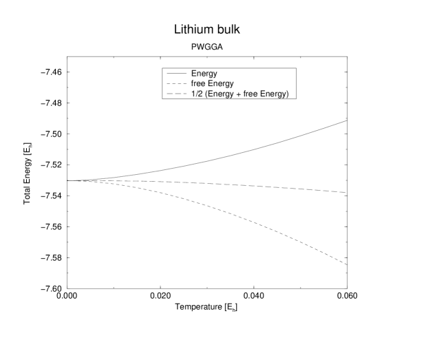
FIG. 1.: Energy $E(T)$, free energy $F(T)$ and $\frac{1}{2}(E(T)+F(T))$ of Li bulk, bcc lattice. A shrinking factor of 16 was used.

In conclusion, as we need a high accuracy for the energy difference between the different phases of Li, we chose for the calculations on lithium bulk a shrinking factor of 16 for the Pack-Monkhorst net which gives 145 sampling points in the irreducible Brillouin zone of the non-distorted bulk and a temperature of 0.001 $E_{h}$. This ensures that convergence of the energy to at least $10^{-4}E_{h}$ with respect to reciprocal space sampling is achieved.

III Results for bulk Lithium

A Band structure

FIG. 2.: LDA band structure at the equilibrium lattice constant, bcc lattice

In figure 2 the LDA band structure for the bcc structure is displayed. The occupied bands and the lower unoccupied bands are in excellent agreement with results earlier obtained with Gaussian basis sets and $X_{\alpha}$ exchange [37], by the Kohn-Korringa-Rostoker (KKR) method [38] and Slater exchange, augmented plane wave (APW) [39] and modified APW (MAPW) [15] calculations both using LDA, or linear muffin tin orbital (LMTO) calculations [40] with a combination of exchange using the Langreth and Mehl functional [41] and LDA correlation. When using PWGGA instead of LDA, the band structure does not exhibit major differences. The experimentally known conduction band width ($\sim$ 4 eV) [42] is slightly lower than the result calculated here (4.6 eV). The slow decay of the density matrix in metals leads to difficulties when Fock exchange is involved: the summation of the exchange series in direct space is very long ranged and is truncated at a large but finite distance. This cutoff for large distances in direct space results in numerical instabilities for small $\vec{k}$. Thus, both in the Hartree-Fock and B3LYP band structures, artificial oscillations can be found around the Gamma point. As usual for Hartree-Fock calculations, we find that the bandwidth is roughly twice as large as the experimental bandwidth.

B Cohesive properties

Table III gives results for ground state properties of bcc Li (lattice constant, bulk modulus, cohesive energy and elastic constants C₁₁, $C_{11}-C_{12}$, and C₄₄). The elastic constants were obtained by applying a rhombohedral distortion for $C_{44}$, a tetragonal distortion for $C_{11}$, and an orthorhombic distortion for $C_{11}-C_{12}$ to the solid at the equilibrium lattice constant. Cohesive energy and lattice constant agree well with experiment and depend only weakly on the basis set. The bulk modulus is obtained from the energy as a function of volume and agrees within the accuracy of the fit with that obtained using the relation $B=\frac{1}{3}(C_{11}+2C_{12})$. Elastic constants have a strong dependence on the basis set and the deviation from experiment improves especially when going from $[3s2p]$ to $[4s3p]$; the $d$-function has only minor impact on the results. We find that PWGGA is closer to experiment with results similar to Ref. [4].

C Relative stabilities

The experimental crystal structure of lithium at zero temperature is still unclear (at room temperature a bcc structure is favoured). Both face-centered cubic (fcc) and hexagonal (hex) structures have been suggested as well as more sophisticated structures such as 9R (a nine layer sequence of close-packed planes ABCBCACAB) [43] or mixtures of these phases. Therefore, we also investigated the relative stability of the different phases. In Figure 3, total energies of bcc, fcc and hex phase, obtained with the PWGGA functional and the best basis set ($[4s3p1d]$), are displayed.

FIG. 3.: Relative stabilities of the different phases as a function of volume, $[4s3p1d]$ basis.

The c/a ratio of the hexagonal phase remains close to the ideal close packed value of 1.633 (it varies between 1.631 and 1.635 which is within the accuracy of the fit). We find that the closed-packed structures are slightly lower in energy than the bcc structure. Although it is reasonable to conclude that the close packed structures are lower in energy than bcc it is not possible to resolve the difference in energy between the fcc and hex phases. The variation of the energy with basis set is given in table IV. As the basis set is systematically improved the energy difference between bcc and fcc increases from 1 $\times 10^{-5}E_{h}$ to 4 $\times 10^{-5}E_{h}$, and between bcc and hex decreases from 7 $\times 10^{-5}E_{h}$ to 4 $\times 10^{-5}E_{h}$. We note that even the $d$-function influences this energy splitting. These results, which do not include the zero point energy, indicate a preference for closed-packed structures which is in agreement with most of the previous calculations [4, 5, 6, 7, 8, 9, 10, 11, 12, 13, 14] except for one [15] (see table IV).

HF calculations were only possible with the smallest $[3s2p]$ basis set where the order of phases is different with hcp being the lowest in energy, followed by bcc and fcc being highest. The same is found in LDA with the smallest $[3s2p]$ basis set, but changes when the basis set is increased to $[4s3p]$ where both fcc and hcp are 2 $\times 10^{-4}E_{h}$ lower in energy than bcc (again, calculations with the best $[4s3p1d]$ basis set were not possible because of linear dependence) — table IV.

As the energy splitting between the close packed and bcc phases is rather small the zero-point energy difference cannot be neglected. The first published calculation of this, based on the harmonic approximation, [5] gave an additional stabilization of $9\times 10^{-5}E_{h}$ of the fcc phase compared to the bcc phase. In these calculations however the hcp phase was found to be higher in energy that the bcc phase (table IV). Very recently, in a calculation also including anharmonic effects, the stabilization was calculated to be about $1.5\times 10^{-5}E_{h}$ both for fcc and 9R phases relative to the bcc phase [6]. In addition, the authors computed the variation of the vibrational free energy as a function of temperature and found a phase transition from a closed packed to a bcc phase at a temperature of $T\sim 200K$.

IV Results for surfaces

A further test of this approach is the calculation of surface energies. We model lithium surfaces by using a slab and varying the numbers of layers (a bcc structure is assumed). Surface energies can be calculated in two ways, either by deriving a bulk energy by subtracting energies of two slabs with $n$ and $m$ layers:

$$E_{surface}=\frac{1}{2}(E_{slab}(n)-(E_{slab}(n)-E_{slab}(n-m))\frac{n}{m})$$ (1)

which has the advantage of a systematic error cancellation (in particular the reciprocal space sampling is consistent between the bulk and slab energies) or by using an independent bulk energy

$$E_{surface}=\frac{1}{2}(E_{slab}(n)-E_{bulk}\times n)$$ (2)

All the quantities $E_{surface}$, $E_{slab}(n)$, and $E_{bulk}$ are energies per atom.

In Figure 4, results for surface energies using both equation 1 (with $m$=1) and 2 are displayed. Equation 1 leads to relatively strong oscillations (dotted line with pluses) and gets more stable the larger $m$. Numerical noise in the expression $(E_{slab}(n)-E_{slab}(n-m))\frac{n}{m}$ is reduced for larger values of $m$. Equation 2, however, leads at zero temperature to a slight linear decreasing of the surface energy as a function of the number of layers (thin line without additional symbol). The reason for the nonvanishing slope is that the energy difference $E(n)-E(n-1)$ is not identical to the energy of the bulk due to the systematic errors in the convergence of the total energy with respect to reciprocal lattice sampling (this was also emphasized in Refs. [16, 17]). As shown in table II, at zero temperature the bulk energy is still changing on the order of $10^{-4}E_{h}$ with increasing sampling point number. Similarly the bulk energy varies when extracted from the slab. This slight discrepancy gives rise to a variation of the surface energy with the number of layers with a slope of $10^{-4}E_{h}/atom/layer$.

The origin of the poor convergence with respect to reciprocal lattice sampling is due to the sharp cutoff imposed by the Fermi energy. One possibility to obtain the surface energy would be to use the intercept from a linear fit, but a better and simpler way to alleviate the difficulties associated with reciprocal lattice sampling is smearing the Fermi surface with a finite temperature. Already at a temperature of 0.001 $E_{h}$, the slope is virtually zero (thick line without additional symbol). This is consistent with table II as the bulk energy converges much faster at finite temperature. At a higher temperature of $k_{B}T=0.02E_{h}$, $E(T)$ clearly deviates from $E(0)$ (thin line with stars) and the approximation $E(0)=\frac{1}{2}(E(T)+F(T))$ should be applied. This works very well when comparing the corresponding results (thin line with crosses) with results calculated at $k_{B}T=0.001$ $E_{h}$ (thick line without additional symbol). The surface energy obtained this way is only slightly higher than that from a calculation at $k_{B}T=0.001$ $E_{h}$ which is consistent with figure 1.

A higher smearing temperature also reduces the oscillations in the curves both when using equation 1 or 2. It even allows to substantially reduce the number of sampling points as shown in Figure 5. At low temperature, a high number of sampling points is necessary to obtain the correct result whereas at high temperature already a shrinking factor of 4 (resulting in 6 sampling points in the irreducible zone) is sufficient. It should be noted that in this case we used Equation 1 so that all the data is consistently extracted from calculations on slabs.

In conclusion, calculations at zero temperature are very cumbersome when results from calculations on slabs and on the bulk have to be combined. The error cancellation can be maximized by extracting the surface energy from calculations on slabs only. The problem of error cancellation between bulk and slab is already improved at very low temperature when it is possible to fully converge the bulk energy with respect to reciprocal lattice sampling. Higher temperature also leads to a smoother behaviour of the surface energy as a function of number of layers. Finally, calculations at high temperature can be performed with a strong reduction of the number of sampling points and using $E(0)=\frac{1}{2}(E(T)+F(T))$ as an approximation for zero temperature results as suggested in Ref. [36].

In table V, LDA and PWGGA results for the unrelaxed (100), (110) and (111) surface are summarized. The lattice constant was chosen as the bulk equilibrium lattice constant, a temperature of 0.001 $E_{h}$ and a higher shrinking factor of 24 resulting in 91 sampling points for the slabs and 413 sampling points for the bulk was used.

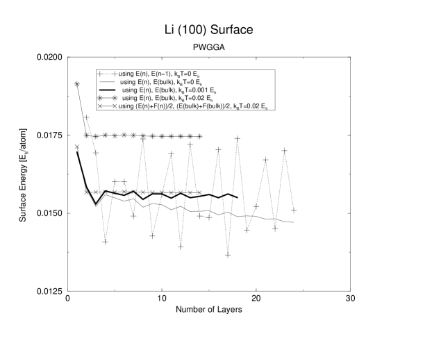
FIG. 4.: (100) Lithium surface energy with a shrinking factor of 24 in the Pack-Monkhorst net, $[3s2p]$ basis.

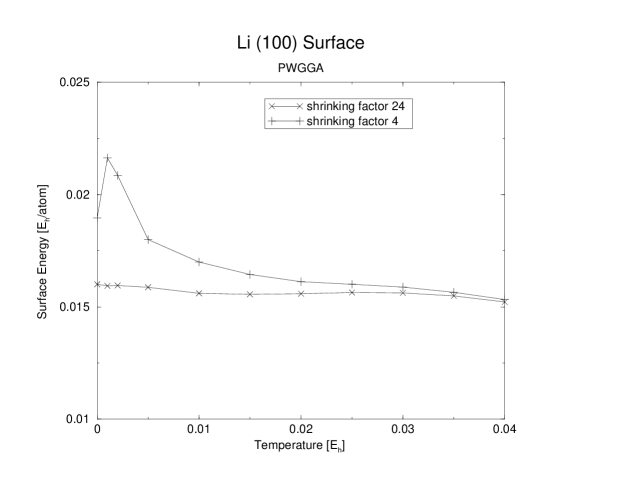
FIG. 5.: (100) Lithium surface energy with two different reciprocal lattice samplings extracted from two slabs with 5 and 6 layers using $\frac{1}{2}(E(T)+F(T))$ and Equation 1

As found in Ref. [4] for the jellium model without additional long-range corrections, surface energies in PWGGA are lower than in LDA (the different lattice constants for PWGGA and LDA are not the reason, an evaluation at the LDA equilibrium lattice constant leads to a change of the PWGGA surface energy which is negligible compared to the difference between LDA and PWGGA surface energies). The energies are reduced when going from the smaller $[3s2p]$ to the $[4s3p]$ basis set, introducing a $d$ function leads only to minor changes. Our results agree well with the literature [16, 44].

V Conclusion

In this study of lithium metal, we presented accurate results using a full potential, all electron density functional scheme. Results for cohesive properties, elastic constants, band structure, and surface energies are in full agreement with experiment and calculated values from literature. The results in best agreement with experiment were obtained with the gradient corrected functional of Perdew and Wang. Hartree-Fock calculations for lithium are very difficult as it is impossible to optimize the exponents because of the very long range of the exchange interaction; the same problems appear in functionals involving an admixture of Fock exchange. We demonstrated the convergence of the different properties with respect to the computational parameters by using an hierarchy of basis sets, different reciprocal lattice samplings and different smearing temperatures. We showed that finite temperature calculations can be used to improve convergence and still an extrapolation to zero temperature is possible and accurate. Quantities like cohesive energy and lattice constant are already stable with the smallest basis set; elastic constants and surface energies are more sensitive. The most difficult quantity to calculate is the energy splitting between the different phases where we have reached the limit of numerical accuracy. We can not make a prediction about the preferred crystal structure; the energy difference is so small that, from the computational point of view, even subtle changes such as introducing a $d$-function are important and zero point energies must be included [5, 6]. We confirm the finding of Ref. [20] that an approach based on Gaussian type functions provides a reliable and very efficient description of metallic systems.

TABLE I.: Basis sets

	exponent	$s$ contraction	$p$ contraction	$d$ contraction
$[1s]$	840.0	0.00264
	217.5	0.00850
	72.3	0.0335
	19.66	0.1824
	5.044	0.6379
	1.5	1.0
$[3s2p]$
$[2sp]$	0.50	1.0	1.0
$[3sp]$	0.10	1.0	1.0
$[4s3p]$ and $[4s3p1d]$
$[2sp]$	0.50	1.0	1.0
$[3sp]$	0.20	1.0	1.0
$[4sp]$	0.08	1.0	1.0
$[d]$	0.15			1.0

TABLE II.: Convergence of the total energy with respect to the number of sampling points. The results are obtained from PWGGA calculations with a $[3s2p]$ basis set, for the bcc lattice at a lattice constant of 3.44 Åand for three temperatures 0 $E_{h}$, 0.001 $E_{h}$, and 0.02 $E_{h}$.

shrinking	number of	Shrinking factor of Gilat net
factor of the	sampling points in	in multiples of shrinking factor
Pack Monkhorst	irreducible part of the	of the Pack-Monkhorst net
net	Pack-Monkhorst net
$k_{B}T=0E_{h};E(T)=E(0)$
		1	2	3	4
4	8	-7.520822	-7.520213	-7.520284	-7.520373
8	29	-7.527049	-7.529923	-7.530344	-7.530488
12	72	-7.528987	-7.529867	-7.530023	-7.530075
16	145	-7.529574	-7.530032	-7.530125
18	195	-7.529697	-7.530077
20	256	-7.529796	-7.530101
24	413	-7.529915	-7.530130
$k_{B}T=0.001E_{h};E(T)$
4	8	-7.524523	-7.522697	-7.521528	-7.521029
8	29	-7.529710	-7.530632	-7.530634	-7.530654
12	72	-7.529982	-7.530156	-7.530141	-7.530128
16	145	-7.530175	-7.530183	-7.530181
18	195	-7.530195	-7.530189
20	256	-7.530185	-7.530188
24	413	-7.530200	-7.530185
$k_{B}T=0.001E_{h};E(0)=\frac{1}{2}(E(T)+F(T))$
4	8	-7.524782	-7.522773	-7.521551	-7.521064
8	29	-7.529759	-7.530653	-7.530658	-7.530674
12	72	-7.530024	-7.530175	-7.530161	-7.530150
16	145	-7.530203	-7.530204	-7.530201
18	195	-7.530218	-7.530211
20	256	-7.530208	-7.530210
24	413	-7.530220	-7.530205
$k_{B}T=0.02E_{h};E(T)$
4	8	-7.521660	-7.516254	-7.515090	-7.514714
8	29	-7.523669	-7.524181	-7.524207	-7.524218
12	72	-7.523698	-7.523670	-7.523664	-7.523661
16	145	-7.523697	-7.523689	-7.523687
18	195	-7.523697	-7.523701
20	256	-7.523697	-7.523701
24	413	-7.523697	-7.523698
$k_{B}T=0.02E_{h};E(0)=\frac{1}{2}(E(T)+F(T))$
4	8	-7.529537	-7.524058	-7.522959	-7.522615
8	29	-7.530824	-7.531214	-7.531234	-7.531242
12	72	-7.530840	-7.530824	-7.530820	-7.530818
16	145	-7.530840	-7.530833	-7.530831
18	195	-7.530840	-7.530842
20	256	-7.530840	-7.530843
24	413	-7.530840	-7.530840

TABLE III.: Ground state properties of lithium. Energies are in $E_{h}$, lattice constants in Å, elastic constants in GPa.

	$a$	$E_{coh}$	$B$	C44	C11	$C_{11}-C_{12}$
LDA ([3s2p])	3.37	0.066	16	13	18	3.2
LDA ([4s3p])	3.40	0.066
PWGGA ([3s2p])	3.44	0.059	14	12	17	3.4
PWGGA ([4s3p])	3.46	0.059	12	12	13	3.5
PWGGA ([4s3p1d])	3.46	0.059	11	12	13	3.3
HF	3.65	0.020	12
Lit. (LDA ; PWGGA, FP-LAPW) [4]	3.37 ; 3.44		15.0 ; 13.4
Lit. (LDA, FP-LAPW) [7]	3.36		15.4		17	2.3
Lit. (LDA, Gaussian basis) [45]	3.45	0.062	13.8
Lit. (LDA, plane wave basis) [5]	3.44		13.5
Lit. (LDA, plane wave basis) [8]	3.40		13.0
Lit. (LDA, Gaussian basis, KSG model) [9]	3.49	0.044	14.7
Lit. (LDA, Gaussian basis, HL model) [9]	3.36	0.062	-
Lit. (LDA, Gaussian basis, RSK model) [9]	3.34	0.068	15.8
Lit. (LDA, HL) [46]	3.39	0.061	14.8
Lit. (MAPW) [15]	3.33	0.074	15.6
Lit. (HF) [23]		0.010 (estimated HF limit: 0.019)
Lit. (HF) [47]	3.65	0.022	14
Lit. (QMC) [47]	3.56	0.058	13
Lit. (local Ansatz) [48]	3.56	0.057	12
exp.	3.48 [49]	0.061 [50]	13.0 [51]	11.6 [51]	14.5 [51]	2.4 [51]

Acronyms are:
Full-potential linear augmented plane wave (FP-LAPW)
Rajaporal-Singhal-Kimball (RSK)
Kohn-Sham-Gaspar (KSG)
Hedin-Lundquist (HL)
Quantum Monte-Carlo (QMC)

TABLE IV.: Relative stability of the different phases of lithium. Energies are in $mE_{h}$ units per atom relative to the bcc phase, lattice constants in Å, bulk moduli in GPa. In the 9R and hexagonal structures the lattice constant $a$ refers to the nearest neighbour distance in the basal plane.

phase	$a$	$E_{bcc}-E$	$B$
fcc, HF ([3s2p])	4.59	-0.08a	12
hcp, HF ([3s2p])	3.24	0.18a	12
fcc, LDA ([3s2p])	4.25	-0.02a	16
fcc, LDA ([4s3p])	4.24	0.19a
hcp, LDA ([3s2p])	3.00	0.08a	16
hcp, LDA ([4s3p])	3.00	0.24a
fcc, PWGGA ([3s2p])	4.33	0.01a	14
fcc, PWGGA ([4s3p])	4.35	0.04a	12
fcc, PWGGA ([4s3p1d])	4.36	0.04a	11
hex, PWGGA ([3s2p])	3.06	0.07a	14
hex, PWGGA ([4s3p])	3.08	0.06a	12
hex, PWGGA ([4s3p1d])	3.08	0.04a	11
fcc, Ref. [4], LDA; PWGGA	4.23; 4.33	0.15; 0.14	15.5; 13.3
fcc, Ref. [6], LDA	4.28 ; 4.32b	0.073 ; 0.057b
hcp, Ref. [6], LDA	3.03	0.062
9R, Ref. [6], LDA	3.03 ; 3.06b	0.065 ; 0.050b
fcc, Ref. [7], FP-LAPW	4.23	0.08	15.2
fcc, Ref. [5], LDA	4.34	0.09 ; 0.18b	13.4
hcp, Ref. [5], LDA	3.09	-0.01	13.3
9R, Ref. [5], LDA	3.07	0.02	13.3
fcc, Ref. [8], LDA	4.28	0.1	13.8
hex, Ref. [8], LDA	3.02	0.33	13.7
fcc, Ref. [9], KSG model	4.38	0.25	18.7
fcc, Ref. [9], RSK model	4.20	0.45	16.8
fcc, Ref. [10], FP-LAPW		0.12
hcp, Ref. [10], FP-LAPW		0.16
fcc, Ref. [11], APW	4.21	1.4
fcc, Ref. [11], FP-LAPW	4.24	0.24
fcc, Ref. [12], LMTO		0.12
hcp, Ref. [12], LMTO		0.15
fcc, Ref. [15], MAPW	4.21	-0.13	12.0

^a As explained in the text, the energy difference is so small that it can only be viewed as a tendency towards closed-packed systems. A statement about the preferred phase is not possible.
^b Including zero point motion.

TABLE V.: Surface energies of (100), (110), and (111) surface, in units of$\frac{mE_{h}}{a_{bohr}^{2}}$; 1 $\frac{mE_{h}}{a_{bohr}^{2}}$=1.5567 $\frac{J}{m^{2}}$

surface	LDA (3.37 Å)	PWGGA (3.44 Å)			Ref. [16] (LDA, 3 layers, at 3.41 Å)
	$[3s2p]$	$[3s2p]$	$[4s3p]$	$[4s3p1d]$
(100)	0.41	0.37	0.30	0.30	0.33
(110)	0.42	0.37	0.32	0.32	0.35
(111)	0.49	0.44	0.34	0.36	0.40

REFERENCES

- [1] C. S. Barrett, Acta Crystallogr. 9, 671 (1956).
- [2] H. G. Smith, R. Berliner, J. D. Jorgensen, M. Nielsen, and J. Trivisonno, Phys. Rev. B 41, 1231 (1990).
- [3] W. Schwarz and O. Blaschko, Phys. Rev. Lett. 65, 3144 (1990).
- [4] J. P. Perdew, J. A. Chevary, S. H. Vosko, K. A. Jackson, M. R. Pederson, D. J. Singh, and C. Fiolhais, Phys. Rev. B 46, 6671 (1992).
- [5] P. Staikov, A. Kara, T. S. Rahman, J. Phys.: Condensed Matter 9, 2135 (1997).
- [6] A. Y. Liu, A. A. Quong, J. K. Freericks, E. J. Nicol, and E. C. Jones, Phys. Rev. B 59, 4028 (1999).
- [7] V. L. Sliwko, P. Mohn, K. Schwarz, and P. Blaha, J. Phys.: Condensed Matter 8, 799 (1996).
- [8] M. M. Dacorogna and M. L. Cohen, Phys. Rev. B 34, 4996 (1996).
- [9] J. C. Boettger and S. B. Trickey, Phys. Rev. B 32, 3391 (1985).
- [10] J. A. Nobel, S. B. Trickey, P. Blaha, and K. Schwarz, Phys. Rev. B 45, 5012 (1992).
- [11] M. Sigalas, N. C. Bacalis, D. A. Papaconstantopoulos, M. J. Mehl, and A. C. Switendick, Phys. Rev. B 42, 11637 (1990).
- [12] J. C. Boettger and R. C. Albers, Phys. Rev. B 39, 3010 (1989).
- [13] H. L. Skriver, Phys. Rev. B 31, 1909 (1985).
- [14] D. A. Young and M. Ross, Phys. Rev. B 29, 682 (1984).
- [15] H. Bross and R. Stryczek, phys. stat. sol. (b) 144, 675 (1987).
- [16] K. Kokko, P. T. Salo, R. Laihhia, and K. Mansikka, Phys. Rev. B 52, 1536 (1995); K. Kokko, P. T. Salo, R. Laihhia, and K. Mansikka, Surf. Science 348, 168 (1996).
- [17] J. C. Boettger and S. B. Trickey, Phys. Rev. B 45, 1363 (1992); J. C. Boettger, Phys. Rev. B 49, 16798 (1994).
- [18] C. Pisani, R. Dovesi, and C. Roetti, Hartree-Fock Ab Initio Treatment of Crystalline Systems, edited by G. Berthier et al, Lecture Notes in Chemistry Vol. 48 (Springer, Berlin, 1988).
- [19] Quantum-Mechanical Ab-initio Calculation of the Properties of Crystalline Materials, Editor: C. Pisani, Lecture Notes in Chemistry Vol. 67 (Springer, Berlin, 1996).
- [20] I. Baraille, C. Pouchan, M. Causà, and F. Marinelli, J. Phys. C 10, 10969 (1998).
- [21] V. R. Saunders, R. Dovesi, C. Roetti, M. Causà, N. M. Harrison, R. Orlando, C. M. Zicovich-Wilson crystal 98 User’s Manual, Theoretical Chemistry Group, University of Torino (1998).
- [22] R. Dovesi, C. Pisani, F. Ricca, and C. Roetti, Phys. Rev. B 25, 3731 (1982).
- [23] R. Dovesi, E. Ferrero, C. Pisani, and C. Roetti, Z. Phys. B 51, 195 (1983).
- [24] M. Prencipe, A. Zupan, R. Dovesi, E. Aprà, and V. R. Saunders, Phys. Rev. B 51, 3391 (1995).
- [25] P. A. M. Dirac, Proc. Cambridge Phil. Soc. 26, 376 (1930); J. C. Slater, Phys. Rev. 81, 385 (1951).
- [26] J. P. Perdew and A. Zunger, Phys. Rev. B 23, 5048 (1981).
- [27] M. W. Schmidt and K. Ruedenberg, J. Chem. Phys. 71, 3951 (1979).
- [28] P. J. Stephens, F. J. Devlin, C. F. Chabalowski, and M. J. Frisch, J. Phys. Chem. 98, 11623 (1994).
- [29] A. D. Becke, Phys. Rev. A 38, 3098 (1988).
- [30] A. D. Becke, J. Chem. Phys. 98, 5648 (1993).
- [31] S. H. Vosko, L. Wilk, M. Nusair, Can. J. Phys. 58, 1200 (1980).
- [32] C. Lee, W. Yang and R. G. Parr, Phys. Rev. B 37, 785 (1988).
- [33] J. D. Pack and H.J. Monkhorst, Phys. Rev. B 16, 1748 (1977).
- [34] N. D. Mermin, Phys. Rev. 137, A 1441 (1963).
- [35] C. L. Fu and K. M. Ho, Phys. Rev. B bf 28, 5480 (1983).
- [36] M. J. Gillan, J. Phys. C 1, 689 (1989).
- [37] W. Y. Ching and J. Callaway, Phys. Rev. B 9, 5115 (1974).
- [38] M. J. Lawrence, J. Phys. F 1, 836 (1970).
- [39] D. A. Papaconstantopoulos et al, http://cst-www.nrl.navy.mil/database.html
- [40] T. Kotani and H. Akai, Phys. Rev. B 52, 17153 (1995).
- [41] D. C. Langreth and M. J. Mehl, Phys. Rev. B 28, 1809 (1983).
- [42] R. S. Crisp and S. E. Williams, Phil. Mag. 5, 525 (1960).
- [43] A. W. Overhauser, Phys. Rev. Lett. 53, 64 (1984).
- [44] H. L. Skriver and N. M. Rosengaard, Phys. Rev. B 11, 7157 (1992).
- [45] J. Callaway, X. Zou, D. Bagayoko, Phys. Rev. B 27, 631 (1983).
- [46] J. F. Janak, V. L. Moruzzi, and A. R. Williams, Phys. Rev. B 12, 1257 (1975).
- [47] G. Yao, J. G. Xu, and X. W. Wang, Phys. Rev. B 54, 8393 (1996).
- [48] A. Heilingbrunner and G. Stollhoff, J. Chem. Phys. 99, 6799 (1993).
- [49] M. S. Anderson and C. A. Swenson, Phys. Rev. B 31, 668 (1985).
- [50] K. A. Gschneidner, Jr., Solid State Phys. 16, 276 (1964).
- [51] R. A. Felice, J. Trivisonno, D. E. Schuele, Phys. Rev. B 16, 5173 (1977).