The steady state quantum statistics of a non-Markovian atom laser

Abstract

We present a fully quantum mechanical treatment of a single-mode atomic cavity with a pumping mechanism and an output coupling to a continuum of external modes. This system is a schematic description of an atom laser. In the dilute limit where atom-atom interactions are negligible, we have been able to solve this model without making the Born and Markov approximations. When coupling into free space, it is shown that for reasonable parameters there is a bound state which does not disperse, which means that there is no steady state. This bound state does not exist when gravity is included, and in that case the system reaches a steady state. We develop equations of motion for the two-time correlation in the presence of pumping and gravity in the output modes. We then calculate the steady-state output energy flux from the laser.

I Introduction

Since the experimental realisation of a Bose Einstein condensate (BEC) in a weakly interacting gas [1, 2, 3, 4], there has been a lot of interest in using similar techniques to produce a superior source for atom optics experiments, which are limited by the linewidth of thermal atomic sources. It was seen that to produce an atom laser, it was simply necessary to generate a BEC and then coherently couple it to the outside world [5, 6, 7, 8, 9, 10, 11, 12, 13, 14]. This was first achieved with sodium atoms at MIT by coupling a BEC from a magnetically trapped state to an untrapped state using an rf pulse [15], and has since been repeated with long rf pulses [16] and Raman transitions [17]. Although the resultant matter waves have been the most monoenergetic source of atoms that have yet been produced, a gain-narrowed atom laser produced with a continuous pumping mechanism will have a spectral density which is orders of magnitude larger. In this paper we will describe a fully quantum mechanical model for such an atom laser which does not make the (invalid) Born or Markov approximations, and also does not make the mean field approximation.

While a condensate is held in a trap, it is in an eigenstate of the system, and is therefore completely monoenergetic. If the trap is suddenly turned off or the condensate is quickly coupled into free space, then the resulting wavepacket will have a spread in energies due to the momentum spread of the trapped wavefunction. Such a coupling tends to conserve momentum. Coupling the atoms out slowly will tend to preserve the energy of the intial state, so a monoenergetic output will be achieved, but this is at the cost of reducing the atomic flux [16, 17, 18]. A continuously pumped laser can have the best of both worlds. Due to a competition between the pumping and the damping, it can produce an increasingly narrow energy spectrum in the output as the pumping and the output flux are increased. It is this feature that we wish to discover in our atom laser model. Several theoretical models of a continuously pumped atom laser have been produced [5, 6, 7, 8, 9, 10, 11, 12, 13, 14], but they have all made the Born and Markov approximations for the output coupling, which have since been shown to be invalid unless the output coupling rate is extremely small [18, 19, 20]. In this paper we produce and solve a model for a continuously pumped atom laser which does not make these approximations.

The early atom laser models are largely distinguished by their choice of cooling method, which was either some form of optical cooling [5, 7, 8], or evaporative cooling [6, 9]. Evaporative cooling appears to be less appropriate for a continuous process, but it is the only method which has experimentally reached the quantum degenerate regime in BEC experiments. In all of these schemes, the model for the damping of the cavity was the same as that used in the master equation for the optical laser. The resulting equations were therefore very similar to optical laser equations. This means that they could be solved using similar methods, and were shown to produce analogous behaviour. We show here that a correct description of the output coupling leads to an irreducibly non-Markovian damping, and can lead to different behaviour.

In an attempt to produce a more realistic description of the output coupling, we modelled a cavity from which atoms were coupled to free space via Raman transitions [14]. This allowed high intensities, spatial control and the possibility of giving the atoms a momentum kick from the lasers, which gave the outcoupled beam a direction. This was recently achieved by Hagley et al. [17]. We also suggested placing the beam in an atomic waveguide such as a hollow optical fibre, which is a possible method of achieving good spatial properties, and an effectively one dimensional output. Although the rate equations and the practicalities of the Raman coupling scheme appeared favourable, it was necessary to produce a more complete theory in order to describe its full effects.

A quantum mechanical theory for the output coupling from an atomic cavity connected to an external field was then developed [18]. This theory described the dynamics of a BEC which is coupled to the outside world, but is not pumped by some continuous process. It was based on the optical input-output formalism developed by Gardiner and Collett [21], but it was complicated by the dispersive nature of the atomic field as compared to the linear energy spectrum for optical fields in free space. A general solution for the dynamics of the cavity and the external fields was presented in terms of Laplace transforms, and an analytical solution was found for a simple form of the coupling [19].

The quadratic nature of the dispersion relations in free space make the dynamics of atom-optical output coupling very similar to those of photon emission in materials with a photonic band gap. Near the edges of these bands, the dispersion relations are quadratic rather than linear, and this causes the model to behave in a non-Markovian way. The same qualitative behaviour was found in treatments of this system as we found in our purely damped case for the atom laser [22, 23].

A complete model of an atom laser must also include the effect of interatomic interactions and a pumping mechanism. The effects of atom-atom interactions are included implicitly in the output coupling models which describe the fields using the nonlinear Schrödinger equation (NLSE), which includes the effect of s-wave scattering [24, 25, 26, 27]. These models based on the NLSE do not consider the effect of the coherences between the lasing mode and the external modes, and therefore implictly made a Born approximation. In fact, all mean-field models are essentially semiclassical models, as they assume that the atoms in the lasing mode can be described by a spatial wavefunction with a predetermined set of quantum statistics. This makes it impossible to fully describe the behaviour of the pumping, and the dephasing of the laser mode must be added a posteriori. The full quantum mechanical description allows us to calculate the quantum statistics using a microscopic model and physical parameters, and therefore allows us to calculate the linewidth of the resulting output.

Unfortunately, interatomic interactions are very difficult to include in a full quantum mechanical model. We present a model of an atom laser which includes a pumping mechanism but assumes that atom-atom interactions are negligible. By making this approximation we have been able to model the output coupling without making the Born-Markov approximation, which is invalid in most physicially relevant parameter regimes. This is an accurate description of very dilute systems, and we show that it can be made self consistently with a laser operating well above threshold, as the threshold can be less than $10^{2}$ atoms in the laser mode [28]. This restriction is made for calculational purposes rather than as a deliberate design criterion. The inclusion of the atom-atom interactions in full generality would require a multimode description of the intracavity field. As discussed above, the mean-field methods which have been so successful in simplifying this procedure cannot be used without destroying the very information that we are trying to find.

It may even be possible to use the single-mode approximation for the cavity after the system has reached a steady state, if this mode is derived self consistently. At this time, the number of atoms in the cavity may be reasonably well defined, and the complicated dynamics of the pumping process may be approximated by a linearised master equation term, as may be constructed for an optical laser [29].

Section II describes our model of a pumped and damped single-mode atomic cavity, and descibes the method by which we may determine the properties of the output field if we know the dynamics of the mode in the cavity. Section III shows how the solution behaves in the absence of pumping. Section IV derives the equations of motion for the system in the presence of pumping and discusses the physics of the various limits of the equations. We see that we can write the equations of motion for the intracavity field in terms of the intracavity operators only, but that this leads to non-Markovian equations. In Sec. V, we show how these equations can be solved to find the two-time correlation of the lasing mode. Section VI shows how the solution in the absence of gravity can be found largely analytically, and that it is not self consistent as a steady state solution. Section VII describes the features of the energy spectrum of the output of an atom laser in the presence of gravity. In Sec. VIII we discuss the possibilities for extending this model.

II The model

We model the atom laser by separating it into three parts. The lasing mode is an atomic cavity with large energy spacing, and when it is operating in the quantum degenerate regime, it is effectively single-mode [8, 14]. We assume that the cavity is single-mode, with annihilation (creation) operator $a^{({\dagger})}$ and a Hamiltonian $H_{s}$. The external field has a different electronic state from the atoms, so the atoms are no longer necessarily affected by the trapping potential. We model the external modes with the field operators $\psi^{({\dagger})}(x)$ and the Hamiltonian $H_{o}$. The operators $a$ and $\psi(x)$ satisfy the normal boson commutation relations. The coupling between the lasing mode and the output modes will be described by the Hamiltonian $H_{i}$. The pump reservoir is coupled to the cavity by an effectively irreversible process. At this stage, we will describe the pump by the Hamiltonian $H_{p}$, which also couples the atoms from a pump reservoir into the system mode.

The total Hamiltonian is then written

$$H_{tot}=H_{p}+H_{s}+H_{i}+H_{o}$$ (1)

where

$$H_{s} = \hbar\omega_{o}a^{{\dagger}}a,$$ (2)

$$H_{i} = i\hbar\int_{-\infty}^{\infty}dx\;(\kappa(x,t)\;\psi(x)a^{{\dagger}}-\kappa(x,t)^{*}\;\psi(x)^{{\dagger}}a)$$ (3)

and where

$$[H_{o},H_{(s,p)}]=[H_{o},a^{({\dagger})}]=[H_{(s,p)},\psi^{({\dagger})}(x)]=0,$$ (4)

as the pump does not directly couple to the external modes. This is described in Fig. 1.

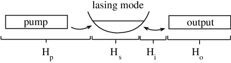
FIG. 1.: Schematic model of the atom laser

We then enter the interaction picture, leaving only $H_{i}$. This gives us the interaction Hamiltonian:

$$H_{int} = i\hbar\int_{-\infty}^{\infty}dx\;(\kappa(x,t)\;\psi_{I}(x,t)a_{I}^{{\dagger}}(t)-$$ (6)

$$\;\;\;\;\;\;\;\;\;\;\;\;\;\;\;\;\;\;\;\;\;\kappa(x,t)^{*}\;\psi_{I}(x,t)^{{\dagger}}a_{I}(t))$$

where

$$\psi_{I}(x,t) = e^{iH_{o}(t-t_{0})/\hbar}\;\psi(x,t_{0})\;e^{-iH_{o}(t-t_{0})/\hbar}$$ (7)

$$a_{I}(t) = e^{i/\hbar(H_{s}+H_{p})(t-t_{0})}\;a(t_{0})\;e^{-i/\hbar(H_{s}+H_{p})(t-t_{0})}$$ (8)

are the system and output field operators in the interaction picture.

We therefore obtain

$$H_{int}=-i\hbar\left(\xi(t)\;a_{I}^{{\dagger}}(t)-\xi^{{\dagger}}(t)\;a_{I}(t)\right)$$ (9)

where $\xi(t)=\int dx\;\kappa(x,t)\psi_{I}(x,t)$.

Appendix A shows how we can go to the Heisenberg picture, and find the result

$$\psi_{H}(x,t)=\psi_{I}(x,t)-\int_{t_{0}}^{t}ds\;F(x,t-s)a_{H}(s)$$ (10)

where $\psi_{H}(x,t)$ and $a_{H}(t)$ are the Heisenberg operators corresponding to $\psi(x)$ and $a$ respectively, and where

$$F(x,t,s) = [\psi_{I}(x,t),\xi^{{\dagger}}(s)]$$ (11)

$$= \int dy\;\kappa^{*}(y,s)[\psi_{I}(x,t),\psi_{I}^{{\dagger}}(y,s)]$$ (12)

$$= \int dy\;\kappa^{*}(y,s)G(x,t,y,s)$$ (13)

where $G(x,t,y,s)$ is the Greens function propagator due to the output Hamiltonian, $H_{o}$, only. These functions can be written in closed form for several useful cases including: free space, free space with gravity, and a repulsive Gaussian potential. We may use Eq. 10 to calculate any observable in the output field that we desire, providing we know the complete history of the system, $a_{H}(s)$. This is a simplified version of the input-output relations for an atomic cavity.

A Output field energy spectrum from $\langle a^{{\dagger}}(t)a(t^{\prime})\rangle$

When the system is in a steady state, we are not interested in the external spectrum directly, as it is always growing. The quantity of interest is the output energy flux. We transform our interaction Hamiltonian into the basis of the energy eigenstates of the output modes:

$$H_{o} = \int dp\;\hbar\>\omega_{p}c_{p}^{{\dagger}}c_{p}$$ (14)

$$H_{i} = i\hbar\;\int dp\;\left(\bar{\kappa}(p,t)\>c_{p}\>a^{{\dagger}}-\bar{\kappa}(p,t)^{*}\>c_{p}^{{\dagger}}\>a\right)$$ (15)

where $c_{p}$ is the annihilation operator associated with the eigenstate of $H_{o}$ that has a position space wavefunction $u_{p}(x)$ and energy $\hbar\omega_{p}$, and where $\bar{\kappa}(p,t)=\int dx\;u_{p}(x)\>\kappa(x,t)$.

We can then write the output energy flux in terms of the two-time correlation of the system.

$$\frac{d\langle c_{p}^{{\dagger}}c_{p}\rangle}{dt}=2\;|\bar{\kappa}(p)|^{2}\;\Re{\left(\int_{0}^{t}du\;e^{-i\omega_{p}(t-u)}\langle a^{{\dagger}}(t)a(u)\rangle\right)}.$$ (16)

This assumes that at time $t=0$, the output field was in the vacuum state.

When the output field is in free space and the only term in $H_{o}$ is the kinetic energy, then the eigenstates are the momentum eigenstates. In this case, $\bar{\kappa}(p,t)$ is just the Fourier transform of $\kappa(x,t)$. When there is a gravitational field, the eigenstates are Airy functions with a displacement which depends on the energy:

$$u_{p}(x)={\cal N}\mbox{Ai}[\beta(x-\frac{\hbar\>\omega_{p}}{m\>g})]$$ (17)

where $\mathcal{N}$ is a normalisation constant, and the length scale is given by $\beta=(2m^{2}g/\hbar^{2})^{1/3}$. In this case $\bar{\kappa}(p,t)$ must be calculated numerically.

We will now derive equations of motion for the system in the absence of pumping.

III Solution in the absence of pumping

When the cavity is not connected to the pump reservoir, we can find the Heisenberg equations of motion for the system operator, and then use Eq.(10) to replace $\psi_{H}(x,t)$ with system operators:

$$\dot{a}(t) = -i\omega_{o}a(t)+\int dx\;\kappa(x,t)\times$$ (19)

$$\;\;\;\;\;\;\;\left(\psi_{I}(x,t)-\int_{t_{0}}^{t}ds\;F(x,t,s)a(s)\right)$$

$$= -i\omega_{o}a(t)-\int_{t_{0}}^{t}ds\;f(t,s)a(s))+\xi(t)$$ (20)

where

$$f(t,s)=\int dx\;\kappa(x,t)F(x,t,s).$$ (21)

For most physical situations, the memory functions $F(x,t,s)$ and $f(t,s)$ are simply functions of $(t-s)$, which means that Eq.(20) is a Volterra equation of convolution type and can be solved using Laplace transforms if the Laplace transform of $f$ exists. This has been solved analytically for simple forms of the coupling in earlier work [18, 19]. In the limit where the decay of the system operator $a(t)$ becomes slow compared to the decay of the memory function, the system operator can be taken out of the integral. This is a Markov approximation, and leads to exponential decay of the trapped mode. The general solution approaches the Markov solution as the strength of the coupling is turned down. Coupling the atoms out at a finite rate causes a significantly non-exponential decay. The difference between the exact and the Markov solutions is examined in detail in parallel work [20].

The most surprising aspect of the exact solution is that it does not necessarily go to zero in the long time limit. If we continuously couple a single-mode in a trap to free space, then some of the initial population will disperse, but a certain fraction of the initial trapped atoms will remain in a non-dispersing eigenstate of the system and the coupling. Even if a momentum kick is given to the atoms as they are coupled out, the bound eigenstate exists, although in this case it will have a lower occupation.

The mechanism for the production of this bound eigenstate can be best seen in a dressed state picture. In this picture, the mixed state which was originally in free space experiences an attractive quasipotential. Let us find the eigenstate of this system explicitly:

As all of the evolution is coherent and we are not including interatomic interactions, the atoms are acting independently in first quantised picture, and we may use single particle quantum mechanics to describe the eigenstate. The state of the system is then described by a wavefunction

$$|\Psi\rangle=c_{a}|\psi_{a}\rangle+\int dx\psi(x)|x\rangle$$ (22)

where $|\psi_{a}\rangle$ is the lasing mode and $\psi(x)$ is the wavefunction outside the trap in the position basis, $\{|x\rangle\}$.

The full Hamiltonian is

$$H = \hbar\omega_{o}|\psi_{a}\rangle\langle\psi_{a}|+\frac{p^{2}}{2M}$$ (24)

$$+\int dx\;\left(g(x)|x\rangle\langle\psi_{a}|+g^{*}(x)|\psi_{a}\rangle\langle x|\right)$$

where $M$ is the mass of the atom and $g(x)$ is the shape of the coupling. This Hamiltonian can describe a momentum kick on the atoms as they leave the trap by having a Fourier transform of $g(x)$ which is not centred around zero. The trapped eigenstate will be of the form

$$|\psi_{E}\rangle=c_{E}|\psi_{a}\rangle+\int dx\;\psi_{E}(x)|x\rangle.$$ (25)

The eigenvalue equation $H|\psi_{E}\rangle=E|\psi_{E}\rangle$ then leads to the following equations:

$$\int dy\;g^{*}(y)\;\psi_{E}(y)+c_{E}\;\hbar\omega_{o} = E\;c_{E},$$ (27)

$$c_{E}\;g(x)-\frac{\hbar^{2}}{2M}\frac{\partial^{2}\psi_{E}}{\partial x^{2}} = E\;\psi_{E}(x).$$ (28)

These are most easily solved in Fourier space, so we take the Fourier transform of both sides and define the Fourier transforms: $\tilde{g}(k)=1/\sqrt{2\pi}\int dx\;g(x)\exp(-ikx)$, $\tilde{\psi}_{E}(k)=1/\sqrt{2\pi}\int dx\;\psi(x)\exp(-ikx)$. We then show that the eigenvalue solves the equation

$$E=\hbar\omega_{o}-\frac{2M}{\hbar^{2}}\;\int dk\;\frac{|\tilde{g}(k)|^{2}}{k^{2}-\frac{2ME}{\hbar^{2}}}$$ (29)

and the corresponding eigenfunction is

$$\tilde{\psi}_{E}(k)=-\frac{2Mc_{E}}{\hbar^{2}}\frac{\tilde{g}(k)}{k^{2}-\frac{2ME}{\hbar^{2}}}.$$ (30)

These equations can be solved analytically for some forms of the coupling $\tilde{g}(k)$, and in general they can be solved numerically. For reasonable physical parameters, there is a single bound eigenstate with negative energy. As the coupling is reduced, this eigenstate becomes more weakly bound. If there was a gravitational potential in the output field, then we would expect that these bound states would become metastable, and would eventually decay. This can be verified numerically [20]. We would also expect atom-atom interactions to destroy this bound state, and in current experiments this is certainly the case, as the mean field interaction energy is much greater than the initial kinetic energy.

In the following figure, we show that when gravity is added to the model, the bound state does indeed decay. We have chosen a Gaussian coupling with width $\sigma_{k}$, which has the form $g(x)=\hbar\sqrt{\Gamma}\;(2\sigma_{k}^{2}/\pi)^{1/4}\;\exp(-(x\;\sigma_{k})^{2})$. We chose a weak gravitational field so that the short time behaviour is unchanged.

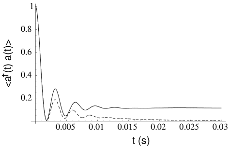
FIG. 2.: This figure shows the decay of the bound state when gravity is introduced. The solid line shows the evolution of the number of atoms in the trap without gravity, and it approaches a steady state value. The dashed line shows how it decays in the presence of gravity ($g=9.8\sin(\pi/20)$). The trap atom number $\langle a^{{\dagger}}(t)a(t)\rangle$ is normalized so that $\langle a^{{\dagger}}(0)a(0)\rangle=1$. Parameters are $\Gamma=10^{6}\mbox{s}^{-2}$, $\sigma_{k}=10^{6}\mbox{m}^{-1}$, $m=5\times 10^{-26}\mbox{kg}$, $\omega_{o}=2\pi\times 123~{}\mbox{s}^{-1}$.

If we solve Eq.(27) and Eq.(28) for this example, we find that there is a bound eigenstate of energy $E/\hbar=-4.3\times 10^{2}s^{-1}$ with $|c_{E}|^{2}=0.34$. This means that $0.34$ of the original state of the system was in the eigenstate, and the rest has gone. It also means that $0.34$ of that remaining eigenstate will be in the trap at any one time. This means that $0.34^{2}=0.12$ of the initial population of the trap will remain in the trap in the long time limit, which is exactly what we see in our simulation.

It is perhaps worth reiterating here that the analysis of this non-Markovian system is almost identical to that found in the field of photonic band gaps. Identical population trapping (in this case photons rather than atoms) has been calculated using identical analytical methods [22, 23]. There are problems in using the Laplace transform method for slightly generalised models, however, even though the equations look almost identical. Particular attention must be paid to the abscissa of convergence, as the Laplace transforms of many physically interesting kernels do not exist at all. A numerical method based on Laplace transforms will give incorrect answers in this case, and alternative methods must be employed.

Gravity is not the only possibility for modelling an output coupling which will eventually remove all of the atoms from the trap. In practice, interatomic interactions may also destroy the stabilty of this state. The largest potential seen by the output atoms other than gravity will be a repulsion from the trapped atoms. This is because the output atoms will be relatively dilute compared to the atoms which remain in the trap. This can be modelled by an external potential for the atoms which will repel them from the trap. We will assume that both of these effects are small so that we can continue to use our single-mode approximation for the lasing state.

The existence of a trapped state when there is no pumping will lead to concern later, as it will mean that pumping will cause the population of the trapped state to increase indefinitely, and no steady state will be reached.

When the model is generalised to include the possibility of pumping, the individual Heisenberg operators $a(t)$ in the two-time correlation can no longer be calculated, so the same techniques for finding a solution do not apply. In the next section we will derive the equation describing the two-time correlation of the cavity field in the presence of pumping.

IV Equations of motion including pumping

If the pump reservoir is sufficiently isolated from the cavity and external fields, and the pumping process is designed to be irreversible, then we may trace over the reservoir states to produce a master equation for a reduced density matrix which describes only the cavity and the external fields. One example of a pumping process which can satisfy these requirements can be found in our earlier model, where cooled atoms in an excited state are passed over the trap containing the lasing mode [14]. The photon emission of the atoms would be stimulated by the presence of the highly occupied ground state, and they will make a transition into that state and emit a photon [30]. For a sufficiently optically thin sample, which can be made possible by having a very tight, effectively low dimensional trap, the photon is unlikely to be reabsorbed, and the process is effectively irreversible. We choose to model an optical cooling process rather than the more experimentally successful evaporative cooling process as we are particularly interested in designing a continuously pumped system with a steady state.

After we have traced over the pump modes, we will produce a term due to the effect of the pump in the master equation for the reduced density matrix $\rho$. It is important to note that we are not tracing over the output field modes, so our reduced density matrix spans the output field as well as the cavity field.

We derive a pumping term based on an approach similar to that followed by Scully and Lamb [31] and found in standard quantum optics texts [29]. We model pumping by the injection of a Poissonian sequence of excited atoms into the atom laser. These atoms may spontaneously emit a photon and make a transition into the atom lasing mode. Alternatively, they may make a transition into other modes of the lasing cavity. For simplicity, we consider an effective two-mode approximation. To obtain the pumping term, we consider the effect of a single atom injected into the atom laser, and then extend this to describe the effect of a distribution of atoms. This gives a master equation describing pumping in the number state basis of the lasing mode $\rho_{nm}=\langle n|\rho|m\rangle$, where each of these elements still include the output field. This equation can be expressed as

$$\left(\dot{\rho}\right)_{\mbox{pump}} = r{\cal D}[a^{{\dagger}}]\left(n_{s}+{\cal A}[a^{{\dagger}}]\right)^{-1}\rho.$$ (31)

where the superoperators ${\cal D}$ and ${\cal A}$ are defined by

$${\cal D}[c] = {\cal J}[c]-{\cal A}[c],$$ (32)

$${\cal J}[c]\rho = c\rho c^{{\dagger}},$$ (33)

$${\cal A}[c]\rho = \frac{1}{2}(c^{{\dagger}}c\rho+\rho c^{{\dagger}}c).$$ (34)

This is the same form as presented for a generic laser master equation by Wiseman [32] where $r$ is the rate at which atoms are injected into the cavity, and $n_{s}$ the saturation boson number. In our particular model $n_{s}$ depends on the ratio of the probability that an atom will spontaneously emit into the lasing mode and the probability that the atom will emit into another mode. This pump process is Markovian for the same reasons that damping in optical lasers is Markovian, as there are photons being lost from the system.

We may write this pumping term in the number basis, $\rho_{n,m}=\langle n|\rho|m\rangle$:

$$\left(\dot{\rho}_{n,m}\right)_{\mbox{pump}} = r\left(\frac{\sqrt{nm}}{n_{s}+(n+m)/2}\rho_{n-1,m-1}\right.$$ (36)

$$\left.-\frac{(n+m+2)/2}{n_{s}+(n+m+2)/2}\rho_{n,m}\right).$$

At this stage, the elements $\rho_{n,m}$ are operators which contain the state of the output modes. For optical lasers, we usually make the Born and Markov approximations at this stage. This is not possible for atom lasers except in extreme parameter limits, but we will review the results than can be obtained with these approximations so that we can compare them with the exact results.

A Pumping using the Born approximation

The Born approximation assumes that the density matrix $\rho$ can be separated into the product of the reduced density matrix for the system $\sigma$, and the reduced density matrix for the output field. It further assumes that the output field remains in its original state. If we then trace over the output field modes, we obtain a master equation for the lasing mode which has the same pumping term as given above [20]. The reduced density now describes only the cavity mode, and $\sigma_{n,m}=\langle n|\sigma|m\rangle$ are c-numbers. The damping term has the form:

$$\left(\dot{\sigma}\right)_{\mbox{damp}} = -\int_{0}^{t}du\;[f(u)e^{i\omega_{o}u}(a^{{\dagger}}a\sigma(t-u)$$ (38)

$$\;\;\;-a\sigma(t-u)a^{{\dagger}})+\mbox{h.c.}]$$

where $f(t)$ has been defined in Eq.(21).

If we combine the pumping and damping terms, we can generate equations of motion for the steady-state atom intracavity number, $p_{n}=\sigma_{n,n}$:

$$\dot{p}_{n}(t) = \frac{rn}{n+n_{s}}p_{n-1}(t)-\frac{r(n+1)}{n+n_{s}+1}p_{n}(t)$$ (41)

$$-2n\int_{0}^{t}du\;\Re(f(u)e^{i\omega_{o}t})p_{n}(t-u)$$

$$+2(n+1)\int_{0}^{t}du\;\Re(f(u)e^{i\omega_{o}t})p_{n+1}(t-u).$$

where $\Re(g)$ is the real part $g$.

By setting the derivatives to zero and assuming that the functions $p_{n}(t)$ approach a constant $p_{n}^{SS}$ as $t$ goes to infinity, we obtain a recursion relation

$$0 = \frac{rn}{n+n_{s}}p_{n-1}^{SS}$$ (44)

$$-\left(\frac{r(n+1)}{n+n_{s}+1}-n\gamma_{BM}\right)p_{n}^{SS}$$

$$+(n+1)\;\gamma\;p_{n+1}^{SS},$$

where

$$\gamma_{BM}=2\int_{0}^{\infty}du\;\Re(f(u)e^{i\omega_{o}u})$$ (45)

which gives us the steady state for the atom number distribution in the cavity:

$$p_{n}^{SS} = {\cal N}\frac{(r/\gamma_{BM})^{n}}{(n+n_{s})!}.$$ (46)

where ${\cal N}$ is a normalisation constant. This form is almost identical to that obtained for the optical laser [29]. The distribution looks thermal for $\alpha=r/\gamma<n_{s}$, and for $\alpha>n_{s}$, which is called the above threshold regime, it approaches a Poissonian distribution with mean atom number $\bar{n}$ and variance $V$ given by:

$$\bar{n} = \frac{r}{\gamma_{BM}}-n_{s},$$ (47)

$$V = \bar{n}+n_{s}.$$ (48)

Eq.(10) will give us the properties of the output field if we can calculate the two-time correlation of the intracavity field. We proceed by finding the equation of motion for the expectation value of the field operator:

$$\left(\frac{d\langle a^{{\dagger}}\rangle}{dt}\right)_{\mbox{pump}} = \sum_{n=0}^{\infty}\sqrt{n}\dot{\rho}_{n-1,n}$$ (49)

$$= \sum_{n=0}^{\infty}\sqrt{n}\rho_{n-1,n}\left(\frac{r}{2n+2n_{s}+1}\right)$$ (50)

$$\approx \frac{r}{2(\bar{n}+n_{s})+1}\langle a^{{\dagger}}\rangle$$ (51)

where we have used the fact that the number distribution is localised to replace $n$ by $\bar{n}$ in the denominator. By expanding the exact expression as a Taylor series in $1/\bar{n}$, we see that there is an error term of the order of $1/\bar{n}^{2}$. This is awkward, as if the first order terms cancel then the linewidth will be of this order. This is in fact what we are hoping to discover, as it will mean that the spectrum will become more narrow as we increase the pumping of the laser. If this occurs, then we may approximate the magnitude of the off-diagonal elements of $\rho$ as though it were a coherent state. We then find that the expression given in Eq. (51) is correct to third order.

The analysis which produced this pumping term was only made possible by assuming that the cavity atom number becomes localised around some mean. If we do not make the Born approximation, then this fact must be taken on faith, and later shown to be a self-consistent solution. Furthermore, if we do not make the Born approximation, then we do not know at this stage what the mean value $\bar{n}$ will be in terms of the other parameters. Once we accept that the atom number distribution peaks around a particular value, however, then we may calculate the output spectrum without having to trace over the output modes.

B Linewidth using the Markov approximation

The Markov approximation can be made in certain physical limits [20]. It corresponds to assuming that the decay of the reservoir correlation function $f(t)$ is fast compared to the rate of change of the density matrix. We wish to describe the atom laser in the parameter regimes where it becomes invalid but we will compare the results of this simple calculation to the results of a calculation which does not make this approxiamtion.

If we make the Born approximation, trace over the output modes and then further assume that a Markov approximation can be made, then we can write the damping term of the master equation as:

$$\left(\dot{\sigma}\right)_{\mbox{damp}} = \gamma_{BM}{\cal D}[a]\sigma.$$ (52)

The derivation of this equation has been examined in detail in other work [20], and it has been assumed to be of this form in earlier atom laser models. It can be generated from Eq.(38) by assuming that $\sigma(t-u)=\sigma(t)$, and can therefore be taken out of the integral. The damping constant $\gamma_{BM}$ is the same as the one defined in Eq.(45).

The total equation of motion for the expectation value becomes

$$\frac{d\langle a^{{\dagger}}\rangle}{dt} = \left(\frac{r}{2(\bar{n}+n_{s})+1}-\frac{\gamma_{BM}}{2}\right)\langle a^{{\dagger}}\rangle$$ (53)

$$= -\frac{r}{4\bar{n}^{2}}\langle a^{{\dagger}}\rangle.$$ (54)

which has an error term proportional to $r/\bar{n}^{3}$.

The solution to this equation is an exponential decay, and the energy spectrum can therefore be shown to be Lorentzian, with a width of $\Gamma=r/(4\bar{n}^{2})$, which is of the order of $\gamma_{BM}/\bar{n}$, and will therefore go to zero as we increase the pumping of the laser. This is called gain-narrowing, and it is a well-recognised feature of the optical laser, but even in optical lasers it is a feature which only exists for certain pumping models. If the pump has a significant response time, then an optical laser can have a linewidth which scales as $r/\bar{n}$, which is simply proportional to the cavity linewidth [29]. Alternatively, a well-designed pump can actually lead to subPoissonian statistics [29].

Since this model of the atom laser exhibits gain-narrowing when we make the Born-Markov approximation, we hope to find that it also exhibits gain-narrowing when we solve the model correctly, as it is this feature which allows the atom laser to produce output with a high spectral density. In Sec. VII we shall show that this is indeed the case.

C Correct treatment of pumping

If we do not make the Born or Markov approximations, but we do assume that the trap population is localised around some (at this stage unknown) value $\bar{n}$, then we can use Eq.(51) to produce a more general equation of motion for the expectation value $\langle a^{{\dagger}}\rangle$:

$$\frac{\partial}{\partial t}\ \langle a^{{\dagger}}\rangle(t)=(i\omega_{o}+P)\langle a^{{\dagger}}\rangle(t)+\int dx\;\kappa^{*}(x,t)\langle\psi^{{\dagger}}\rangle(x,t)$$ (55)

where

$$P=\frac{r}{2(\bar{n}+n_{s})+1}$$ (56)

well above threshold. Remember that we can no longer relate $\bar{n}$ directly to the physical parameters of the problem using Eq.(47), which has used the Born approximation. If the solution exhibits gain-narrowing, then the value of $P$ that we use will actually determine our value of $n_{s}$. We are therefore producing a solution method which can be solved iteratively to produce a self-consistent solution rather than directly generating it.

Under our assumptions the pumping is effectively linear, so we may use the quantum regression theorem. We then recall Eq.(10), and we may immediately derive the following integro-differential equation for the two-time correlation:

$$\frac{\partial}{\partial\tau} \langle a^{{\dagger}}(t+\tau)a(t)\rangle=(i\omega_{o}+P)\langle a^{{\dagger}}(t+\tau)a(t)\rangle$$ (57)

$$\>\>\>\;\;\;-\int_{0}^{t+\tau}du\;f^{*}(t+\tau-u)\langle a^{{\dagger}}(u)a(t)\rangle$$ (58)

where $\tau>0$, and $f(t)$ has been defined in Eq.(21). We have set $t_{0}$ to zero, and assumed that at this point in time there were no atoms in the output field. In other words, at $t=0$ the coupling was switched on, and the expectation values involving the normally ordered operators $\psi_{I}(x,t)$ and $\psi^{{\dagger}}_{I}(x,t)$ will be zero.

This equation is not sufficient to specify the dynamics of the cavity, as it is only a single partial integro-differential equation in a two dimensional space. We also require the integro-differential equation for the intracavity number, which we can generate in a similar manner. Well above threshold, we obtain:

$$\frac{\partial}{\partial t}\langle a^{{\dagger}}a\rangle(t)=r\\ -\int_{0}^{t}du\;2Re\{f^{*}(t-u)\langle a^{{\dagger}}(u)a(t)\rangle\}$$ (59)

These equations are difficult to solve in general, but can be solved simply in various limits. For example, if the kernel $f(t)$ was a $\delta$-function then the equations would become local and the solution would be a simple exponential. This is the case for the Markovian example shown in Sec. IV B above. In the broadband limit of the optical theory, the function $f(t)$ is equivalent to the Fourier transform of a constant, which is exactly a $\delta$-function. Although the broadband limit can be a good approximation for the atomic case as well [19], the fact that atoms will disperse in free space means that the system has an irreducible memory, and is non-Markovian.

D Memory functions

Our model for the output involves a change of electronic state via a Raman transition, which has recently been achieved experimentally[17]. From a specific model of this coupling we can derive the memory functions $f(t,s)$ and $F(x,t,s)$. The form of $f(t,s)$ in this case has also been derived and discussed in the recent work by Jack et al. [33]. In position space, the shape of the coupling will be defined by the shape of the lasers multiplied by an envelope of the spatial wavefunction of the trapped state. For simplicity of calculation, we will assume that the coupling is Gaussian in form, and that there is no net momentum kick given to the atoms. This will allow us to produce analytical forms for the memory functions. Let the coupling be defined by

$$\kappa(x,t)=\sqrt{\gamma}\left(\frac{2\sigma_{k}^{2}}{\pi}\right)^{1/4}e^{-(\sigma_{k}\;x)^{2}}$$ (60)

where $\hbar\sigma_{k}$ is the momentum width of the coupling and $\gamma$ is the strength of the coupling.

In the presence of a gravitational field, $V=mgx$, the Green’s function in Eq.(13) can be found as a standard result [34]:

$$G(x,t,y,s) = \sqrt{\frac{1}{4\pi i\lambda(t-s)}}\times$$ (62)

$$\;\;\;e^{({\frac{i(x-y)^{2}}{4\lambda(t-s)}-\frac{ig(t-s)(x+y)}{4\lambda}-\frac{ig^{2}(t-s)^{3}}{48\lambda}})}$$

where $\lambda=\hbar/(2M)$.

This leads to the following forms for the memory functions:

$$F(x,t,s) = \left(\frac{2}{\pi}\right)^{1/4}\sqrt{\frac{\gamma\>\sigma_{k}}{1-4\>i\>\sigma_{k}\>\lambda\>\Delta t}}\times$$ (64)

$$\;\;\;e^{-\frac{\Delta t\>g(\Delta t^{2}\>g+6\>x)+i\>(\Delta t^{4}\>g^{2}+12\>\Delta t^{2}\>g\>x-12\>x^{2})\>\lambda\sigma_{k}^{2}}{12\>\lambda\>(i+4\>\Delta t\>\lambda\>\sigma_{k}^{2})}}$$

and (65)

$$f(t,s) = \frac{\gamma\;\;\exp({-\frac{g^{2}\>\Delta t^{2}}{32\>\lambda^{2}\>\sigma_{k}^{2}}})\;\;\exp({\frac{-i\>g^{2}\>\Delta t^{3}}{48\>\lambda}})}{\sqrt{1+2\>i\>\lambda\>\Delta t\>\sigma_{k}^{2}}}$$ (66)

where $\Delta t=t-s$.

If we make $g=0$, then we have the memory functions for coupling into free space. We can see that $f(t)$ will then go as $1/\sqrt{t}$ in the long time limit. The broadband limit may also be found by taking $\sigma_{k}\rightarrow\infty$ while $\gamma/\sigma_{k}$ goes to a constant. This limiting case has been examined in detail in previous work [18, 19]. For a non-pumped cavity with a broadband output coupling, the long time limit of the output spectrum has three regimes. In the limit where the coupling is much faster than the free field dispersion rate of the atoms, the energy spectrum looks like the cavity wavefunction which has appeared in free space. In the limit of coupling that is very slow compared to the dispersion rate, the output approaches a Lorentzian. As the coupling strength is increased from one limit to the other, there is a reasonably complex behaviour which at first looks like a deformed Lorentzian, and then produces a fringe-like structure in the spectrum. Eventually, the oscillations decay and the spectrum begins to look like the cavity wavefunction.

There are no useful approximations which can simplify the full calculation. For the purposes of numerical calculations when $g\neq 0$, using the broadband limit is actually less tractable than using the more realistic memory function. This is because the integrals involving $F(x,t,s)$ and $f(t,s)$ become unbounded in amplitude, and their convergence is due to their highly oscillatory nature. Retaining the full form of the equations includes the Gaussian envelope, which defines a natural upper bound to the integrals. Since the oscillations grow rapid on the same scale as this envelope decays, it is probable that the correct solution and the broadband limit are qualitatively very similar.

If the two-time correlation is very slowly changing then it may be removed from the integral in Eq. (58), which is equivalent to approximating the kernel to be extremely narrow. We may therefore guess that well above threshold, where we hope to find a slowly decaying two-time correlation (or a narrow linewidth), the Markov approximation may hold, and the output will be Lorentzian in energy. However, there is also the possibility of other behaviour. Even if the amplitude of the two-time correlation decayed slowly and exponentially, a fast change in the phase of the solution would not only mean that there was a shift in the resonance, but would also significantly change the effective decay constant. There is no obvious way to determine whether the coupling will induce such a rotation without actually solving the original Volterra equation. In fact, we must solve Eq. (58) and Eq. (59) self-consistently to be sure that this system will exhibit gain-narrowing of the output field.

In the next section, we will show how we may find a solution to Eq. (58) and Eq. (59), and then in the following sections we will calculate the output from a laser with $g=0$, and then with a nonzero gravitational field.

V Solution methods

Equation (58) and Eq. (59) do not form a standard pair of partial integro-differential equations. The derivative in Eq. (58) is only defined for $\tau>0$, and so we cannot require that the solution obey this equation through the whole domain of the integral. This means that Eqn. (58) cannot be integrated to find the solution, as we do not actually know the derivative at any point. Since the two-time correlation is Hermitian, we can we rewrite the integral so that the domain remains in the $\tau>0$ plane, but we still do not have a continuously defined derivative along the length of the integral. This is shown graphically in Fig. (3).

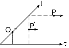
FIG. 3.: The $\tau>0$ half plane of the two-time correlation. Equation (58) defines the horizontal partial derivatives over the entire region, and the domain of the integral corresponding to the derivative at point $P$ is shown with a dashed line. The only derivative known at point $P^{\prime}$ is in the direction shown. Equation (59) defines the derivative along the diagonal, and the domain of the integral corresponding to the derivative at point $Q$ is shown with a dotted line.

We proceed by making an ansatz which uses the solution of Eq. (58) which has been extended into the region $\tau<0$. We then use the $\tau>0$ portion of this solution to substitute into the two-time correlation in Eq. (59). We introduce the function $J(t)$, which is the solution of the equation

$$\frac{\partial J(t)}{\partial t}=(i\omega_{o}+P)J(t)-\int_{0}^{t}dw\;f^{*}(t,w)J(w).$$ (67)

This means that

$$\langle a^{{\dagger}}(t+\tau)a(t)\rangle=\langle a^{{\dagger}}a\rangle(t)\frac{J(t+\tau)}{J(t)}$$ (68)

is a solution of Eq. (58) with the correct initial condition at $\tau=0$. We then substitute this result into Eq.(59):

$$\frac{d\langle a^{{\dagger}}a\rangle(t)}{dt}=r-\int_{0}^{t}dw\;\langle a^{{\dagger}}a\rangle(w)\;\Re{\left(\frac{2f(t,w)J(t)}{J(w)}\right)}.$$ (69)

Solving these two equations gives the two-time correlation for the lasing mode, from which we may find the properties of the output field. It is only consistent with our linearisation of the pumping if the number of atoms in the trap, $\bar{n}$, is stable around the value which originally produced the parameter $P$. Since we require $P$ to generate the solution, and $\bar{n}$ is simply the long time limit of Eq. (69), the effective free parameter is $n_{s}$. This threshold parameter must be much smaller than $\bar{n}$, so we search for a value of $P$ which gives the result $\bar{n}\gg n_{s}$.

Once it is established that Eq. (69) is approaching a stable steady state, a fast way of finding that steady state is to set the derivative to zero, and assume that $\langle a^{{\dagger}}a\rangle(w)=\bar{n}$ over the support of the kernel. This gives

$$\bar{n}=\frac{r}{\int_{0}^{t}dw\;\Re{\left(\frac{2f(t,w)J(t)}{J(w)}\right)}}.$$ (70)

There are many numerical methods for solving Volterra equations, and since $f(t,s)=f(t-s)$, Eq. (58) is of the convolution type, which has many specialised methods of solution. We have found that this equation can be solved analytically by a Laplace transform method in the absence of gravity and in the broadband limit. However, for the more general forms of coupling that we have examined in this paper, even numerical Laplace transform methods become invalid as the Laplace transform of the memory function does not always exist. In these cases we require an alternative numerical method.

We transform Eq. (67) into a rotating frame by introducing the function

$$N(t)=J(t)\;\exp(-i\omega_{o}t-Pt)$$ (71)

and rewriting the equation of motion for $J(t)$ in terms of $N(t)$:

$$\frac{\partial N(t)}{\partial t}=-\int_{0}^{t}dw\;H(t,w)N(w)$$ (72)

where $H(t,w)=f^{*}(t,w)\exp(-[i\omega_{o}+P](t-w))$. Since $f(t,w)$ is actually just a function of $(t-w)$, this equation is of convolution type. Unfortunately, the numerical methods for finding the solution of convolution type Volterra equations depend on the simplicity of the kernel for their effectiveness. We have found that the most effective numerical method for solving this equation is simply a direct integration of Eq. (72) using a second order algorithm for both the integration and the calculation of the integral to find the derivative at each timestep. Such techniques can be found in many common collections of numerical methods [35].

In the following section, we will examine the case where $g=0$, and atoms are simply diffusing away from the trap.

VI Ideal atom lasers must point down

Real atom lasers will be able to point in any direction and still expect a beam of atoms to be emitted. The three reasons for this are repulsive atom-atom interactions which will eject the unconfined atoms, the presence of gravity which will accelerate the atoms away from the lasing mode, and any momentum kick given to the atoms by the coupling process. We shall show that it is not actually possible to produce even an idealised model without either the gravity or the atom-atom interactions.

We will do this by attempting to make a model of an ideal atom laser without considering complicating factors such as atom-atom interactions and gravity. In this limit, we can use analytical methods to solve Eq. (58).

If we take the Laplace transform of Eq. (58), and then use the convolution and derivative theorems, then we obtain

$$J(t)=J(0)\;{\cal L}^{-1}\left\{\frac{1}{s-(i\omega_{o}+P)+{\cal L}\{f^{*}\}(s)}\right\}(t)$$ (73)

where ${\cal L}\{f\}(s)=\int_{0}^{\infty}dt\;f(t)\exp(-st)$ is the Laplace transform of $f(t)$, and ${\cal L}^{-1}$ is the inverse Laplace transform.

When $g=0$ and we go to the broadband limit, then the memory function is

$$f(t)=|\Omega|^{2}(1-i)\frac{1}{\sqrt{\lambda\>t}}$$ (74)

where $\Omega$ is a constant related to the strength of the coupling.

For this form of $f(t)$, we can find the solution to Eq. (73) using results from eariler work [19, 20]. We discover that in the long time limit it grows exponentially. The number of atoms in the cavity also grows exponentially when this solution is substituted into Eq. (59). This shows that for $g=0$, the steady state approximation on which we based our linearisation of the pumping in Sec.(IV C) is not self-consistent.

The exponential growth is not physically realistic, and is merely an artifact of the breakdown of our approximation. In essence, our approximation will ignore the depletion of the pump if the linearisation is not valid and so in that case we would be modelling a pump which can deliver an infinite atomic flux. The reason for the absence of the steady state is clear once we have discovered the existence of the trapped state which was described in Sec.(III). Since our trap does not empty when there no pumping, it is not unreasonable to expect that a certain fraction of the atoms coming into the trap from the pump will enter the trapped state. This will mean that the number of atoms in the cavity would continually grow. We expect that solving this system without linearising the pump would lead to a solution that involved a trap number which increased linearly.

The absence of a steady state means that this model is not suitable for describing an atom laser, and a greater level of detail is required in order for the model to behave realistically. In other words, our idealised atom laser model must be more complete than the idealised optical laser model. We also realise that it is the nature of the output coupling which must be made more realistic. A purely damped cavity must lose all of its atoms in the long-time limit, or there is not really any hope that the pumped atom laser will reach a steady state.

Our examination of the trapped state in Sec.(III) guides us here, as we know that merely adding a momentum kick to the coupling does not remove the trapped state. It is likely that appropriately strong and repulsive interatomic interactions would provide the required realism, but we find that that the effects of a gravitational field are simpler and easier to model. In the next section, we show that an atom laser in a gravitational field does indeed produce a self-consistent steady state.

VII Output from an atom laser

The output from an atom laser where the output atoms accelerate under a uniform gravitational field is a function of many physical parameters. In terms of independent timescales for the dynamics, we can control the dispersion rate in free space (by choosing the mass of the atoms); the time taken for the output atoms to leave the trap due to gravity; the coupling rate between the trap and the output; the pumping rate; the threshold pumping rate and the trap frequency. Within this phase space, we are constrained by physical limits such as the choice of atom and atomic trap. We are also constrained by our operational limits, such as our maximum allowable trap density and our desire to be well above threshold. Finally, we are constrained by computational limits, which make it difficult to calculate the behaviour of the laser when any of these timescales become radically different from the others. In principle it is possible to discover approximations that will work in any of these limits, but each one would have to be considered separately. We will simply examine the behaviour of the output for many different pumping and damping rates. We will choose the remaining parameters as realistically as possible.

The shape of the coupling $\kappa(x,t)$ is determined largely by the spatial wavefunction of the laser mode, and this in turn is a function of the trap energy. We use the trap frequency $\omega_{o}=2\pi\times 123$ Hz, which is near those used in experiments [4]. We use an atomic mass of $m=5\times 10^{-26}$kg and a gravitational field of $g=9.8\sin(0.18)$ m s^-2. We assume the coupling to be Gaussian, with a form given by Eq. (60), and a momentum width $\sigma_{k}=4.4\times 10^{5}$ m^-1.

Our first calculation will show that the system can reach a steady state. We choose a pumping rate of $r=5.0\times 10^{5}$s^-1, and a threshold cavity number of $n_{s}=8$. The damping rate is then chosen so that the number of atoms in the trap will be much larger than $n_{s}$. We use $\gamma=2.0\times 10^{5}$ s^-2, which gives $\bar{n}=1180\gg n_{s}$. We then solve Eq. (72) and use the result to solve Eq. (59), which gives us the number of atoms in the trap as a function of time. The results are shown in Fig. (4), where we can see that after initial transient behaviour, the number of atoms reaches a steady state.

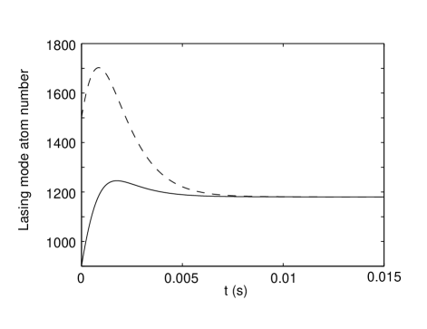
FIG. 4.: This figure shows that the pumped atom laser reaches a steady state when the output field experiences a gravitational field. The solid and dashed lines indicate the solution for different initial trap numbers.

The initial transient behaviour is only correct as a first approximation, as we are actually determining a self-consistent steady state for this system in which the parameter $P$ is stable. The different starting values for $\bar{n}$ are included to demonstrate that this solution can be found in a stable fashion.

The two-time correlation derived in this calculation is approaching an exponential in the long time limit. Unlike the Born-Markov solution, this exponential has a large rotating term. This rotation gives the output a frequency shift and it also alters the integral in Eq. (72) which in turn affects the rate of decay. Even in the strong pumping limit, where the amplitude of the two-time correlation is decaying very slowly, the Markov approximation gives an incorrect result.

In a counterintuitive way, the fact that the Markov approximation is not valid makes it harder to compare the correct calculation to a Born-Markov result. When the memory function is effectively a delta function, then the Markov approximation gives the same result in any rotating frame, but when the memory function doesn’t decay instantaneously, then the decay rate and the frequency shift depend on the rotating frame in which the Markov approximation is made. This is nothing more than saying that the Markov approximation is not self-consistent. For the purpose of being definite, we will use the most “natural” version of a Markov approximation, in which we rotate at the system frequency $\omega_{o}$. This gives the linewidth shown in Sec. IV B and the damping rate given by the Born approximation, Eq. (45).

We now look at what happens when the pumping is increased. We use a damping constant of $\gamma=2.0\times 10^{4}$ s^-2, and a threshold of $n_{s}=47$, and vary the pumping rate. As the pumping rate increases, the steady state number of atoms in the trap increases, and the modulus of the two-time correlation decays more slowly. The energy spectrum of the output flux is proportional to the Fourier transform of the two-time correlation through Eq. (16), so we can see that the energy spectrum is becoming more narrow as the two-time correlation becomes broader. This means that the laser is experiencing gain-narrowing.

In Table 1 we show the results of these calculations. We give the pumping rates $r$ and the resulting mean atom cavity numbers $\bar{n}$. The linewidth of the output energy flux, $\Gamma$, is calculated directly from the two-time correlation using Eq. (16). This is compared to the linewidth given by the Born-Markov approximation $\Gamma_{BM}$, which was found from Eq. (53). The spectral shift $\Delta\omega$ is the amount by which the correct result is shifted from the Born-Markov result. This spectral shift is seen to be largely a function of the damping only, and therefore does not change as we vary the pumping.

We claimed in the introduction that a continuously pumped atom laser can have a linewidth much narrower than can be obtained by dropping the atoms from the trap after a rapid state change. In the fast coupling limit the output field will simply look like the original condensed wavefunction. More precisely, the output field will have the same shape as $\kappa(x)$, which for our example will be a Gaussian, given by Eq. (60). We may proceed to find the energy spectrum by changing to the free space energy basis ($\omega=\lambda k^{2}$). The resulting energy spectrum is

$$|\psi(w)|^{2}=\frac{1}{\sqrt{2\pi\sigma_{k}^{2}\lambda\omega}}\;\exp(\frac{-\omega}{2\lambda\sigma_{k}^{2}}).$$ (75)

which is normalised so that $\int_{0}^{\infty}d\omega\;|\psi(w)|^{2}=1$.

This spectrum is singular, so a FWHM definition of the width would be meaningless. We shall define the linewidth, $\Gamma_{fast}$, obtained by a rapid state change by the equation $\int_{0}^{\Gamma_{fast}}d\omega\;|\psi(w)|^{2}=1/2$. For the parameters used above, this gives us $\Gamma_{fast}=88$ s^-1. Comparing this linewidth to those calculated in Table 1 shows that our atom laser gives an improvement of two to three orders of magnitude in spectral density.

TABLE I.: Linewidth as a function of pumping

$r$ ($10^{3}$/s)	$\bar{n}$	$\Gamma$(s-1)	$\Gamma_{BM}$(s-1)	$\Delta\omega$ (s-1)
20	450	2.1	0.025	0.16
40	910	1.1	0.012	0.15
80	1800	0.56	0.0062	0.14
800	$1.8\times 10^{4}$	0.035	0.00062	0.14

We plot the spectral flux corresponding to three of these pumping rates in Fig. (5). The vertical scale is normalised to the peak height for each plot so that the width of the spectra can be easily compared.

FIG. 5.: The spectra of the output energy flux for three different pumping rates. The solid, dashed and dotted lines represent $r=800$ s^-1, $r=80$ s^-1 and $r=40$ s^-1 respectively. Other parameters are given in Table 1.

Although this line narrowing seems to suggest that the linewidth of the output can be reduced indefinitely, in practice there will be a limit due to technical noise in the pumping, output coupling and the laser mode. A limit due to the finite temperature of the trap has been calculated recently by Graham [37].

From Table 1, we can see that the solution obtained with the Born-Markov approximation is significantly different from the correct solution. In Fig. (6) we plot the output energy spectrum with and without the Born-Markov approximation. We have chosen the parameters $r=5.0\times 10^{5}$ s^-1, $\gamma=2.0\times 10^{5}$ s^-2 and $n_{s}=8$. This example is well above threshold, with a mean atom number of $\bar{n}=1200$. We scale the two solutions so that their peaks are the same height so that they can easily be compared.

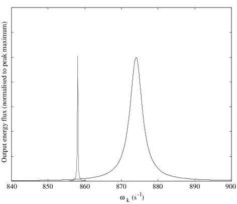
FIG. 6.: The output energy flux spectrum without (solid line) and with (dashed line) the Born-Markov approximation. Parameters are $r=5.0\times 10^{5}s^{-1}$, $\gamma=2.0\times 10^{5}s^{-2}$ and $n_{s}=8$.

VIII Conclusions

We have demonstrated that for some interesting parameter regimes an atom laser cannot be modelled by Markovian equations. Although this was shown earlier for a nonpumped cavity [18, 19, 20], there was some hope that the slowly decaying two-time correlation in the pumped case would resurrect some form of the Markov approximation. We have shown that this can only be true when the coupling is very weak, which will tend to make either the atomic flux very weak, or else require extremely large atomic densities.

For noninteracting atoms, the non-Markovian equations can be solved analytically in the limit of zero pumping, as was the case for the pulsed atom laser [15]. We have developed a numerical method for calculating the output spectrum in the presence of pumping. We have found that when the full, non-Markovian dynamics are considered, it is necessary to add gravity to the model in order for a self-consistent steady state to be produced.

This model does not include atom-atom interactions and therefore only works when the atomic field is very dilute, which is consistent with our parameters. The advantage of this model is that we have calculated the full quantum statistics of the lasing mode, which is impossible with atom laser models which involve nonlinear Schrödinger equations based on mean-field theory. Future work will involve generalising this atom laser model to include some of the effects of interactions without making an initial mean-field approximation. This will allow us to determine the limitations on the coherence of a practical atom laser, and thus the limits on their interferometric applications.

A Deriving the Langevin equation

In this appendix, we derive Eq. (10). This means that we need to find $\psi_{H}(x,t)$, which can be written:

$$\psi_{H}(x,t)=U_{int}^{{\dagger}}(t,t_{0})\;\psi_{I}(x,t_{0})\;U_{int}(t,t_{0}).$$ (A1)

where $U_{int}(t,t_{0})$ is the unitary evolution operator corresponding to the interaction Hamiltonian, Eq (9). It is the identity operator when $t=t_{0}$, and obeys the dynamic equation

$$\frac{\partial U_{int}(t,t_{0})}{\partial t}=\frac{-i}{\hbar}\;H_{int}(t)\;U_{int}(t,t_{0}).$$ (A2)

We proceed in a very similar manner to a calculation made by Jack et al. in their work on non-Markovian quantum trajectories [36]. Let us consider the operator

$$U(t,t_{0})=T_{a}\left\{V_{+}V_{0}V_{-}\right\}(t,t_{0})$$ (A3)

where $T_{a}$ is a time ordering operator which denotes a time ordering on the $a$ operators only, and where we have defined the operators

$$V_{+}(t,t_{0}) = \exp\left(-\int_{t_{0}}^{t}ds\;\xi^{{\dagger}}(s)a_{I}(s)\right)$$ (A4)

$$V_{0} = e^{-\int_{t_{0}}^{t}du\;\int_{t_{0}}^{u}dv\;f(u,v)\;a_{I}^{{\dagger}}(u)a_{I}(v)}$$ (A5)

$$V_{-} = \exp\left(\int_{t_{0}}^{t}ds\;\xi(s)a_{I}^{{\dagger}}(s)\right)$$ (A6)

where $f(u,v)=[\xi(u),\xi^{{\dagger}}(v)]$ is the same function defined in Eq. (21).

Now $U(t_{0},t_{0})$ is clearly the identity operator. The equation of motion for $U(t,t_{0})$ is given by

$$\frac{\partial U(t,t_{0})}{\partial_{t}} = T_{a}\left\{\frac{\partial V_{+}}{\partial t}V_{0}V_{-}\right\}+T_{a}\left\{V_{+}\frac{\partial V_{0}}{\partial t}V_{-}\right\}$$ (A8)

$$\rule{42.67912pt}{0.0pt}+T_{a}\left\{V_{+}V_{0}\frac{\partial V_{-}}{\partial t}\right\}$$

$$= -T_{a}\left\{\xi^{{\dagger}}(t)a_{I}(t)\>V_{+}V_{0}V_{-}\right\}$$ (A11)

$$-T_{a}\left\{V_{+}\>\int_{t_{0}}^{t}ds\;f(t,s)\>a_{i}^{{\dagger}}(t)a_{I}(s)\>V_{0}V_{-}\right\}$$

$$+T_{a}\left\{-V_{+}V_{0}\>\xi^{{\dagger}}(t)a_{I}(t)\>V_{-}\right\}$$

$$= \frac{-i}{\hbar}\;H_{int}(t)\;T_{a}\left\{V_{+}V_{0}V_{-}\right\}(t,t_{0})$$ (A12)

where we used the lemma

$$T_{a}\left\{[V_{+}(t,t_{0}),\xi(t)]\right\}=\int_{t_{0}}^{t}du\;f(t,u)\;a_{I}(u)\;V_{+}(t,t_{0}).$$ (A13)

We therefore see that since $U(t,t_{0})$ obeys the same equation of motion and has the same initial condition as $U_{int}(t,t_{0})$, then it must be the same operator. We use this alternate form of the evolution operator to find $\psi_{H}(x,t)$.

$$\psi_{H}(x,t) = U^{{\dagger}}(t,t_{0})\;\psi_{I}(x,t)\;U(t,t_{0})$$ (A14)

$$= \psi_{I}(x,t)+U^{{\dagger}}(t,t_{0})\;T_{a}\left\{[\psi_{I}(x,t),V_{+}]\>V_{0}V_{-}\right\}$$ (A15)

$$= \psi_{I}(x,t)+U^{{\dagger}}(t,t_{0})\;\times$$ (A17)

$$\;\;\;\;\int_{t_{0}}^{t}ds\;F(x,t,s)\;T_{a}\left\{a_{I}(s)\>V_{+}V_{0}V_{-}\right\}$$

where $F(x,t,s)=[\psi_{I}(x,t),\xi^{{\dagger}}(s)]$ is the same function as defined in Eq (13). We then use the lemma

$$T_{a}\left\{a_{I}(s)\;V_{+}V_{0}V_{-}\right\} = T_{a}\{a_{I}(s)V_{+}(t,s)V_{0}(t,s)V_{-}(t,s)\times$$ (A19)

$$\;\;\;\;V_{+}(s,t_{0})V_{0}(s,t_{0})V_{-}(s,t_{0})\}$$

$$= U(t,s)\;a_{I}(s)\;U(s,t_{0})$$ (A20)

to reach the final form of Eq.(A17):

$$\psi_{H}(x,t) = \psi_{I}(x,t)-\int_{t_{0}}^{t}ds\;F(x,t,s)\;a_{H}(s).$$ (A21)

REFERENCES

- [1] M.H. Anderson et al., Science 269, 198 (1995).
- [2] C.C Bradley et al., Phys. Rev. Lett.75, 1687 (1995).
- [3] K.B. Davis et al., Phys. Rev. Lett.75, 3969 (1995).
- [4] M.O. Mewes et al., Phys. Rev. Lett.77, 416 (1996).
- [5] M. Olshanii, Y. Castin and J. Dalibard, Proc. of the 12th Int. Conference on Laser Spectroscopy, edited by M. Inguscio, M. Allegrini and A. Sasso. (1995).
- [6] M. Holland, et al., Phys. Rev. A 54, R1757 (1996).
- [7] H.M. Wiseman and M.J. Collett, Physics Lett. A 202, 246 (1995).
- [8] R.J.C. Spreeuw et al., Europhysics Letters 32, 469 (1995).
- [9] H.M. Wiseman, A. Martins and D.F. Walls, Quantum Semiclass. Opt. 8, 737 (1996).
- [10] A.G.M. Moore and P. Meystre, Phys. Rev. A53, 977 (1996).
- [11] A.M. Guzman et al., Phys. Rev. A53, 977 (1996).
- [12] U. Janicke and M. Wilkens, Europhys. Lett. 36, 561 (1996).
- [13] C. Bordé, Phys. Lett. A 204, 217 (1995).
- [14] G.M. Moy, J.J Hope and C.M. Savage, Phys. Rev. A55, 3631 (1997).
- [15] M.-O. Mewes et al., Phys. Rev. Lett.78, 582 (1997), M.R. Andrews et al., Science 275, 637 (1997).
- [16] I. Bloch, T.W. Hänsch and T. Esslinger, Phys. Rev. Lett.bf 82, 3008 (1999).
- [17] E.W. Hagley et al., Science 283, 1706 (1999).
- [18] J. Hope, Phys. Rev. A55, R2531 (1997).
- [19] G.M. Moy and C.M. Savage, Phys. Rev. A56, R1087 (1997).
- [20] G.M. Moy, J.J. Hope and C.M. Savage, Phys. Rev. A59, 667 (1999).
- [21] C. Gardiner and M.J. Collett, Phys. Rev. A31, 3761 (1985).
- [22] S. John and T. Quang, Phys. Rev. Abf 50, 1764 (1994).
- [23] N. Vats and S. John, Phys. Rev. A58, 4168 (1998).
- [24] M. Naraschewski, A. Schenzle, and H. Wallis, Phys. Rev. A, 56, 603 (1997).
- [25] H. Steck, M. Naraschewski and H. Wallis, Phys. Rev. Lett.80, 1 (1998).
- [26] W. Zhang and D.F. Walls, Phys. Rev. A57, 1248 (1998).
- [27] B. Kneer et al., Phys. Rev. A58, 4841 (1998).
- [28] J.J. Hope, G.M. Moy, M.J. Collett and C.M. Savage, unpublished.
- [29] see e.g. D.F. Walls and G.J. Milburn, Quantum Optics, Springer-Verlag (1994).
- [30] J.J. Hope and C.M. Savage, Phys. Rev. A54, 3117 (1996).
- [31] M.O. Scully and W.E. Lamb, Phys. Rev. A159, 208 (1967).
- [32] H. Wiseman, Phys. Rev. A56,2068 (1997).
- [33] M.W. Jack, M. Naraschewski, M.J. Collett and D.F. Walls, Phys. Rev. A59, 2962 (1999).
- [34] see e.g. L.Schulman, Techniques and Applications of Path Integration, Wiley (1981).
- [35] see, for example, Numerical Recipes, which can be found at http://www.nr.com
- [36] M.W. Jack, M.J. Collett and D.F. Walls, J. Opt. B, in press.
- [37] R. Graham, Phys. Rev. Lett.81, 5262 (1998).