[

Berry Phase and Ground State Symmetry in $H\otimes h$ Dynamical Jahn-Teller Systems

Abstract

Due to the ubiquitous presence of a Berry phase, in most cases of dynamical Jahn-Teller systems the symmetry of the vibronic ground state is the same as that of the original degenerate electronic state. As a single exception, the linear $H\otimes h$ icosahedral model, relevant to the physics of C₆₀ cations, is determined by an additional free parameter, which can be continuously tuned to eliminate the Berry phase from the low-energy closed paths: accordingly, the ground state changes to a totally-symmetric nondegenerate state.

]

The traditional field of degenerate electron-lattice interactions (Jahn-Teller effect) in molecules and impurity centers in solids[1, 2] has drawn interest in recent years, excited by the discovery of new systems calling for a revision of a number of commonly accepted beliefs. Several molecular systems including C₆₀ ions, higher fullerenes and Si clusters, derive their behavior from the large (up to fivefold) degeneracy of electronic and vibrational states due to the rich structure of the icosahedral symmetry group.[3] Novel Jahn-Teller (JT) systems have therefore been considered theoretically,[2, 4, 5] disclosing intriguing features,[5, 6, 7, 8, 9] often related to a Berry phase[10] in the electron-phonon coupled dynamics.

As it is well known, the molecular symmetry, reduced by the JT distortion with the splitting of the electronic-state degeneracy, is restored in the dynamical Jahn-Teller (DJT) effect, where tunneling among equivalent distortions is considered. The vibronic states are therefore labelled as representations of the original point group of the undistorted system. In the weak-coupling regime, for continuity, the ground state (GS), in particular, retains the same degenerate representation as that labelling the electronic level prior to coupling. A priori, there is no particular reason for this to continue at larger couplings. However, it appears empirically[2] that in all linear DJT systems studied before the late nineties, the GS symmetry remains the same at all couplings. The explanation of this observation was a great outcome of the Berry-phase[10] scenario: the phase entanglement in the electron-phonon Born-Oppenheimer (BO) dynamics,[5, 11, 12, 13] originating at electronically-degenerate high-symmetry points, seemed a universal feature of the DJT systems.

In this context, it came as a surprise the discovery of the first linear JT system showing a nondegenerate GS in the strong-coupling limit:[8, 9] the spherical model ${\cal D}^{(2)}\otimes d^{(2)}$ of electrons of angular momentum $L=2$ interacting with vibrations also belonging to an $l=2$ representation. This system turns out to be a special case of the $H\otimes h$ icosahedral model, for a 5-fold degenerate $H$ electronic state interacting linearly with a distortion mode of the same symmetry $h$.[8, 14] In that special case, it was shown that, for increasing coupling, a nondegenerate $A$ excited state in the vibronic spectrum moves down, to cross the $H$ GS at some finite value of the coupling parameter, thus becoming the GS at strong coupling.[8, 9] This phenomenon is a manifestation of the absence of Berry-phase entanglement in the coupled dynamics.[8, 15]

In this Letter we study the linear $H\otimes h$ model in its generality. We analyse in detail the connection between the symmetry/degeneracy of the vibronic GS and the presence/absence of a Berry phase in the coupled dynamics. This model owns its peculiarities to the non-simple reducibility of the icosahedral symmetry group. In particular, the $H$ representation appears twice in the symmetric part of the Kronecker product of the $H$ representation with itself:

$$\{H\otimes H\}^{(s)}=a\oplus g\oplus h^{[1]}\oplus h^{[2]}\;.$$ (1)

There are, therefore, two independent sets of Clebsch-Gordan (CG) coefficients

$$C_{m_{1},m_{2}}^{m~{}[r]}\;\equiv\;\langle H,m_{1};H,m_{2}|h,m\rangle^{[r]}$$ (2)

for the coupling of an $H$ electronic state with an $h$ vibrational mode, identified by a multiplicity index $r=1,2$.[16] Of course, since the two $h$ states are totally equivalent and indistinguishable, symmetry-wise, the choice of these orthogonal sets of coefficients has some degree of arbitrariness: the free parameter $\alpha$ in the combination

$$C_{m_{1},m_{2}}^{m}\left(\alpha\right)\equiv\cos\alpha~{}C_{m_{1},m_{2}}^{m~{}[1]}+\sin\alpha~{}C_{m_{1},m_{2}}^{m~{}[2]}$$ (3)

accounts for it. The coefficient $C_{m_{1},m_{2}}^{m}\left(\alpha\right)$ coincides with the $r=1$ and $r=2$ values[17] for $\alpha=0$ and $\alpha=\frac{\pi}{2}$ respectively. Also, for $\alpha=-\arctan\left(3/\sqrt{5}\right)\equiv-\alpha_{s}$, it becomes equivalent to the spherical CG coefficient.

The basic Hamiltonian for the $H\otimes h$ model can be written:

$$H=H_{\rm harm}(\hbar\omega)+H_{\rm e-v}(g\hbar\omega,\alpha)\;,$$ (4)

with

$$H_{\rm harm}(\hbar\omega) = \frac{1}{2}\hbar\omega\sum_{m}(p_{m}^{2}+q_{m}^{2})$$ (5)

$$H_{\rm e-v}(g\hbar\omega,\alpha) = \frac{g\hbar\omega}{2}\sum_{m~{}m_{1}m_{2}}q_{m}c^{\dagger}_{m_{1}}c_{-m_{2}}C_{m_{1},m_{2}}^{m}\left(\alpha\right)\;,$$ (6)

where $q_{m}$ is the distortion coordinate (with conjugate momentum $p_{m}$) and $c^{\dagger}_{m}$ is the electronic operator in standard second-quantized notation.

The novelty introduced by the $\alpha$-dependent CG coefficients reflects the fact that the group does not determine completely the form of the linear coupling as, for example, in cubic symmetry. The specific value of this angle must be established case by case by detailed analysis of the phonon mode and its coupling with that specific electronic state. Indeed, in a realistic case such as, for example, C${}_{60}^{+}$ ions, each $h$ mode is characterized not only by its own frequency $\omega_{i}$ and scalar coupling $g_{i}$, but also by its particular angle of mixing $\alpha_{i}$.

For intermediate to strong coupling, the interesting nonperturbative regime, the customary framework is the BO separation of vibrational and electronic motion: when the splitting among the five potential sheets (proportional to $g^{2}$) is large, the electronic state can be safely assumed to follow adiabatically the lowest BO potential sheet, while virtual inter-sheet electronic excitations may be treated as a small correction. The BO dynamics is determined by the lowest eigenvalue of the interaction matrix $\Xi=\sum q_{m}V^{(m)}$ in the electronic space. This matrix is obtained from (6) by the same technique described in Ref. [15]: since it is a simple generalization of that obtained for for ${\cal D}^{(2)}\otimes d^{(2)}$,[15] here for brevity we report only the expression of the diagonal matrix elements of the $V^{(0)}$ matrix, corresponding to the coupling to a pure $q_{0}$ distortion:

$$\left[\matrix{C_{0,2}^{2}\left(\alpha\right)\cr-C_{0,1}^{1}\left(\alpha\right)\cr C_{0,0}^{0}\left(\alpha\right)\cr-C_{0,1}^{1}\left(\alpha\right)\cr C_{0,2}^{2}\left(\alpha\right)\cr}\right]=\cos\alpha\left[\matrix{{\frac{1}{2\,{\sqrt{5}}}}\cr{\frac{1}{2\,{\sqrt{5}}}}\cr{\frac{-2}{{\sqrt{5}}}}\cr{\frac{1}{2\,{\sqrt{5}}}}\cr{\frac{1}{2\,{\sqrt{5}}}}\cr}\right]+\sin\alpha\left[\matrix{-{\frac{1}{2}}\cr{\frac{1}{2}}\cr 0\cr{\frac{1}{2}}\cr-{\frac{1}{2}}\cr}\right]\;.$$ (7)

This form makes it clear that a shift $\alpha\rightarrow\alpha+\pi$ introduces a sign change in the coupling matrix, and it can be compensated by a reflection $\vec{q}\rightarrow-\vec{q}$. We will restrict therefore, without loss of generality, to the interval $0\leq\alpha\leq\pi$.

The electronic eigenvalue $\frac{-2}{{\sqrt{5}}}\cos\alpha$ is the lowest for $\alpha<\alpha_{s}$ and $\alpha>\pi-\alpha_{s}$ (region a): in this range the BO potential presents six absolute minima, one of which is lying along the $\hat{q}_{0}$ pentagonal axis, with energy lowering $E_{\rm clas}=-g^{2}/10~{}\cos^{2}\alpha$ (in units of $\hbar\omega$). However, influenced by the $V^{(m\neq 0)}$ matrices, in the complementary interval $\alpha_{s}<\alpha<\pi-\alpha_{s}$ (region b), ten trigonal distortions become the absolute minima, with energy gain $E_{\rm clas}=-g^{2}/18~{}\sin^{2}\alpha$. At the boundary angles ($\alpha=\alpha_{s}$ and $\pi-\alpha_{s}$), all pentagonal and trigonal minima become degenerate, and part of a continuous degenerate 4-dimensional (4-D) trough[8] of depth $E_{\rm clas}=-g^{2}/28$.

We come now to the rôle of the Berry phase in this system. As well known, the geometrical phase is related to conical degeneracies of the two lowest BO potential surfaces.[6] In the ${\cal D}^{(2)}\otimes d^{(2)}$ system[15] (the $\alpha=\pi-\alpha_{s}$ case of the model studied here) the flat minimum trough presents tangentially degenerate points. For that case, it was shown that the tangential contacts provide a mechanism for getting rid of the Berry phase.[15, 18] For generic $\alpha$ instead, all contacts between the lowest two potential sheets occur as conic intersections, instead of tangencies, at points which are far from the potential minima. In particular, both trigonal and pentagonal axes are locations of conical crossings for $\alpha$ in regions a and b respectively (i.e. when they do not correspond to minima). In particular, for $\vec{q}$ on the $\hat{q}_{0}$ axis, the five electronic eigenvalues are given in Eq. (7), where it can be readily verified that for $\alpha$ in region b the most negative one is indeed twofold degenerate.

In region a, the six minima are all equidistant, defining the simplest regular polytope in 5 dimensions (see Fig. 1a). In this case, therefore, minimal closed paths join any of the 20 triplets of minima. It is straightforward to verify that at the center of all such triplets there lies one of the trigonal axes, carrying a conical intersection. If the degeneracy were restricted to the trigonal axes, however, the rich topology of the 5-D space would allow the triangular loop to squeeze continuously to a point avoiding the degenerate line: the associated Berry phase would then vanish. Instead, we checked that the two lowest sheets remain in contact through a bulky 3-D (1 radial + 2 tangential) region of distortions surrounding each trigonal axis. This guarantees the nontrivial topology of the loops, thus the possibility of nonzero Berry phase. Indeed a geometrical phase of $\pi$ is associated to these triangular loops, as we computed explicitly by the discretized phase integral of Ref. [19]. Paths encircling two (or any even number) of such triangles (thus looping through 4, 6,… minima) have zero Berry phase, since the two phases cancel out. However, such paths, though energetically equivalent to the basic triangles (since they cross the same saddle points), are longer, therefore less relevant from a minimum-action point of view. We conclude consequently that, for $\alpha$ in region a, the $H\otimes h$ model must show the signature of a Berry-phase entanglement.

In region b, the minima are ten, each with 3 nearest neighbors and 6 second neighbors. The shortest closed paths through minima joins three points such as (1$\rightarrow$2$\rightarrow$3$\rightarrow$1) in Fig. 1b. However, energetically, such loop is not the most convenient, since the segment joining two far neighbors (3$\rightarrow$1) must cross a barrier energetically 60% more expensive than that linking next neighbors (1$\rightarrow$2). Since the energy gaps between minima and saddle points grow as $g^{2}$, eventually at strong coupling only the “cheapest” paths affect the low-energy dynamics, and the relevant Berry phases should be calculated along such loops. Here, therefore, at large $g$, the low-energy paths are pentagons, such as (1$\rightarrow$2$\rightarrow$3$\rightarrow$4$\rightarrow$5$\rightarrow$1) in Fig. 1b. We computed the Berry phases for both kinds of paths, obtaining $\pi$ and $0$ for the 3-points and 5-points loop respectively. This implies that the pentagonal loop encircles an even number (most likely 6) of degenerate regions (one of which around the pentagonal axis at the center of each 5-points loop), each carrying a phase factor $e^{i\pi}$. We conclude that, in region b, although nontrivial Berry phases are present, they have no effect on the strong-coupling low-energy spectrum. Thus, in particular, the GS symmetry should remain $H$ in region a, while a nondegenerate $A$ state must turn lower in region b at strong coupling. We stress that we have established the presence of nonzero Berry phases for all values of $\alpha$, but also that, in region b, the effect of the geometrical phase is bypassed by energetically cheaper paths with null phase.

This scenario is confirmed by numerical diagonalization (Lanczos method).[8, 20] In Fig. 2, we plot the gap between the lowest $H$ and $A$ vibronic states, wherever $E_{H}-E_{A}>0$, and 0 where the GS is $H$. At weak coupling, as suggested by continuity, the GS is $H$. For $g>7$ and $\alpha$ in range b, the $A$ state becomes the GS. We note however a little modulation in the boundaries of this region, both $g$- and $\alpha$-wise. We observe, in particular, that the two special values $\alpha_{s}$ and $\pi-\alpha_{s}$, far from marking the closing of the $H-A$ gap, show instead a rather sharp peak in the $\alpha$ direction. By drawing (in Fig. 2) the gap multiplied by $g^{2}$, we evidence, along these ridges at $\alpha_{s}$ and $\pi-\alpha_{s}$, the $g^{-2}$ large-$g$ behavior of the $H-A$ gap, characteristic of the motion in a flat trough of size $\sim g$. Inside the region b, instead, the gap vanishes much more quickly, due to the tunnelling integral through the barriers between trigonal minima vanishing exponentially in $g^{2}$.

It is straightforward to extend the one-mode Hamiltonian (4) to a more realistic case of many distortion modes,[21] each characterized by its own frequency, coupling and angle of mixing:

$$H=\sum_{i}\left[H_{\rm harm}(\hbar\omega_{i})+H_{\rm e-v}(g_{i}\hbar\omega_{i},\alpha_{i})\right]\;.$$ (8)

We study in detail the two-modes case. Five free parameters ($\omega_{1}$ being taken as a global scale factor) appear in the model. In order to carry out a significant study of the phase diagram, we limit ourselves to (i) two values only (1 and 5) of the ratio $\omega_{2}/\omega_{1}$,[22] and (ii) $\alpha_{2}-\pi/2=\alpha_{1}\equiv\alpha$, assuming a principle of ”maximum difference” between the modes. We take advantage of spectral invariance for individual sign change of each of the couplings $g_{i}\rightarrow-g_{i}$ and for $\alpha\rightarrow-\alpha$, restricting to the $0\leq\alpha\leq\pi/2$, $g_{i}>0$ sector. For convenience, we introduce polar variables $g_{1}=g\cos\gamma$, $g_{2}=g\sin\gamma$ ($0<\gamma<\pi/2$), and draw slices of the parameters space for fixed values of $g$, as $\alpha-\gamma$ planes.

The first interesting observation concerns the case of equal frequencies: even though Hamiltonian (8) is linear in the coupling parameters the CG coefficients and the boson operators, the special case $\omega_{1}=\omega_{2}$ cannot be trivially reduced to a one-mode problem, by means of a suitable rotation mixing mode 1 and 2. This is a consequence of the linear independence of the coupling matrices $V^{(m)}(\alpha)$ for different values of $\alpha$.

We resort to exact diagonalization to treat the two-modes case. Due to the larger size of the matrices, we are limited to smaller couplings: we obtain a satisfactorily converged $E_{H}-E_{A}$ gap up to $g\lesssim 10$ only. The calculations, for both $\omega_{2}/\omega_{1}=1$ and 5, show that for $g\leq 7$ the GS symmetry remains $H$ for any $\alpha$ and $\gamma$ as in the one-mode case. Then, already at $g=8$, an $A$ (nondegenerate) GS makes its appearance in two localized regions of the $\alpha-\gamma$ plane. Starting from $g\gtrsim 9$, these separated regions assume essentially their asymptotic strong-coupling shape (see Fig. 3). The first region, located symmetrically across $\alpha=\pi/2$, corresponds mainly to mode 1 with b-type (no-Berry) coupling: mode 2 (Berry-phase entangled in this region) acts as a weak perturbation, incapable to change the GS symmetry for small enough $\gamma$. On the other side, the second region of $A$ GS is located around $\alpha=0$: there, it is mode 2 who is responsible for the no-Berry phase coupling, mode 1 acting as a weak perturbation, for $\gamma$ close enough to $\pi/2$. For $\omega_{2}/\omega_{1}=1$ (not reported here), the two $A$-GS regions are, of course, equivalent. For $\omega_{2}/\omega_{1}=5$ (Fig. 3) instead, these two regions differ in size, in relation with the different relative energetics of mode 1 versus mode 2.

In conclusion, we have illustrated the importance of the energetics of paths surrounding the points of degeneracies of the two lowest BO potential sheets, for defining the effective rôle of the Berry phase. In all classical linear JT models, the low-energy paths are affected by the geometrical phase in a way leading to a “boring” fixed ground-state symmetry. The $H\otimes h$ model is special in being determined by an additional parameter, allowing to change the connectivity of the graph of low-energy paths through minima along with the regions of degeneracy of the two lowest sheets. Consequently, this new parameter leads continuously from a regular, Berry-phase entangled, region to a whole region where, although present, the Berry phase is totally ineffective in imposing its selection rules to the low-energy vibronic states, and to the GS in particular.

Finally, for a system such as C${}_{60}^{+}$ our study implies that a detailed knowledge of not only the coupling parameters $g_{i}$, but also the characteristic angles $\alpha_{i}$ should be acquired for all modes in order to compute even such a basic property as the GS symmetry.

We thank Arnout Ceulemans, Brian Judd, Fabrizia Negri, Erio Tosatti, and Lu Yu for useful discussions.

FIG. 1.: The connectivity of the BO potential minima for regions a and b of angle $\alpha$ introduced in the text. All lines (solid and dashed) join nearest neighbor minima.

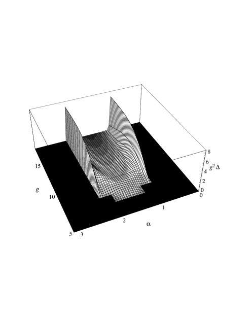
FIG. 2.: $g^{2}$ times the gap $\Delta=E_{H}-E_{A}$ (units of $\hbar\omega$, logarithmic gray-scale) between the lowest non-$G$ and non-$A$ vibronic states as a function of $g$ and $\alpha$. In the positive region, the GS is $A$, elsewhere it is $H$. This generates on the $g-\alpha$ plane a zero-temperature “phase diagram”. The basis is truncated to include up to 40 oscillator states.

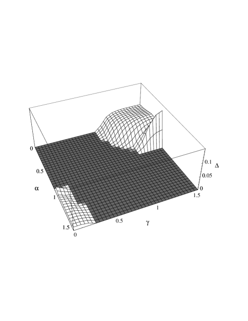
FIG. 3.: The gap (units of $\hbar\omega_{1}$) between the lowest non-$G$ and non-$A$ vibronic states as a function of $\alpha$ and $\gamma$ (defined in the text), for $g=10$, $\omega_{2}/\omega_{1}=5$. In the positive region, the GS is $A$, elsewhere it is $H$. The basis includes up to 12 oscillator states, enough to give a fairly converged value of $\Delta=E_{H}-E_{A}$.

REFERENCES

- [1] R. Englman, The Jahn Teller Effect in Molecules and Crystals (Wiley, London, 1972).
- [2] I. B. Bersuker and V. Z. Polinger, Vibronic Interactions in Molecules and Crystals (Springer Verlag, Berlin, 1989).
- [3] E. Lo and B. R. Judd, Phys. Rev. Lett. 82, 3224 (1999).
- [4] J. Ihm, Phys. Rev. B 49, 10726 (1994).
- [5] A. Auerbach, N. Manini, and E. Tosatti, Phys. Rev. B 49, 12998 (1994) . Phys
- [6] C. A. Mead, Rev. Mod. Phys. 64, 51 (1992).
- [7] Geometric Phases In Physics, edited by A. Shapere and F. Wilczek (World Scientific, Singapore, 1989).
- [8] P. De Los Rios, N. Manini and E. Tosatti, Phys. Rev. B 54, 7157 (1996).
- [9] C. P. Moate, M. C. M. O’Brien, J. L. Dunn, C. A. Bates, Y. M. Liu, and V. Z. Polinger, . Rev. Lett 77, 4362 (1996).
- [10] M. V. Berry, Proc. R. Soc. Lond. A 392, 45 (1984).
- [11] F. S. Ham, Phys. Rev. Lett. 58, 725 (1987).
- [12] S. E. Apsel, C. C. Chancey, and M. C. M. O’Brien, Phys. Rev. B 45, 5251 (1992).
- [13] M. C. M. O’Brien, Phys. Rev. B 53, 3775 (1996).
- [14] A. Ceulemans, and P. W. Fowler, J. Chem. Phys. 93, 1221 (1990).
- [15] N. Manini and P. De Los Rios, J. Phys.: Condens. Matter 38, 8485 (1998) .
- [16] P. H. Butler, Point Group Symmetry Applications (Plenum, New York, 1981).
- [17] We shall stick here to Butler’s convention,[16] and choose the indexes, labelling states within the degenerate representations, by the algebraic chain of subgroups .
- [18] P. De Los Rios and N. Manini, in Recent Advances in the Chemistry and Physics of Fullerenes and Related Materials: Volume 5, edited by K. M. Kadish and R. S. Ruoff (The Electrochemical Society, Pennington, NJ, 1997), p. 468.
- [19] R. Resta, Rev. Mod. Phys. 66, 899 (1994).
- [20] N. Manini and E. Tosatti, in Recent Advances in the Chemistry and Physics of Fullerenes and Related Materials: Volume 2, edited by K. M. Kadish and R. S. Ruoff (The Electrochemical Society, Pennington, NJ, 1995), p. 1017.
- [21] N. Manini and E. Tosatti, Phys. Rev. B 58, 782 (1998).
- [22] The diagram for yields also the ground-state symmetry for the case , with and exchanged (i.e ) and .