The Quantum Hall Effect:
Novel Excitations and Broken Symmetries

These lectures are dedicated to the memory of Heinz Schulz, a great friend and a wonderful physicist.

Chapter 1 The Quantum Hall Effect

1.1 Introduction

The quantum Hall effect (QHE) is one of the most remarkable condensed-matter phenomena discovered in the second half of the 20th century. It rivals superconductivity in its fundamental significance as a manifestation of quantum mechanics on macroscopic scales. The basic experimental observation is the nearly vanishing dissipation

$$\sigma_{xx}\rightarrow 0$$ (1.1)

and the quantization of the Hall conductance

$$\sigma_{xy}=\nu\frac{e^{2}}{h}$$ (1.2)

of a real (as opposed to some theorist’s fantasy) transistor-like device (similar in some cases to the transistors in computer chips) containing a two-dimensional electron gas subjected to a strong magnetic field. This quantization is universal and independent of all microscopic details such as the type of semiconductor material, the purity of the sample, the precise value of the magnetic field, and so forth. As a result, the effect is now used to maintain the standard of electrical resistance by metrology laboratories around the world. In addition, since the speed of light is now defined, a measurement of $e^{2}/h$ is equivalent to a measurement of the fine structure constant of fundamental importance in quantum electrodynamics.

In the so-called integer quantum Hall effect (IQHE) discovered by von Klitzing in 1980, the quantum number $\nu$ is a simple integer with a precision of about $10^{-10}$ and an absolute accuracy of about $10^{-8}$ (both being limited by our ability to do resistance metrology).

In 1982, Tsui, Störmer and Gossard discovered that in certain devices with reduced (but still non-zero) disorder, the quantum number $\nu$ could take on rational fractional values. This so-called fractional quantum Hall effect (FQHE) is the result of quite different underlying physics involving strong Coulomb interactions and correlations among the electrons. The particles condense into special quantum states whose excitations have the bizarre property of being described by fractional quantum numbers, including fractional charge and fractional statistics that are intermediate between ordinary Bose and Fermi statistics. The FQHE has proven to be a rich and surprising arena for the testing of our understanding of strongly correlated quantum systems. With a simple twist of a dial on her apparatus, the quantum Hall experimentalist can cause the electrons to condense into a bewildering array of new ‘vacua’, each of which is described by a different quantum field theory. The novel order parameters describing each of these phases are completely unprecedented.

We begin with a brief description of why two-dimensionality is important to the universality of the result and how modern semiconductor processing techniques can be used to generate a nearly ideal two-dimensional electron gas (2DEG). We then give a review of the classical and semi-classical theories of the motion of charged particles in a magnetic field. Next we consider the limit of low temperatures and strong fields where a full quantum treatment of the dynamics is required. After that we will be in a position to understand the localization phase transition in the IQHE. We will then study the origins of the FQHE and the physics described by the novel wave function invented by Robert Laughlin to describe the special condensed state of the electrons. Finally we will discuss topological excitations and broken symmetries in quantum Hall ferromagnets.

The review presented here is by no means complete. It is primarily an introduction to the basics followed by a more advanced discussion of recent developments in quantum Hall ferromagnetism. Among the many topics which receive little or no discussion are the FQHE hierarchical states, interlayer drag effects, FQHE edge state tunneling and the composite boson [1] and fermion [2] pictures of the FQHE. A number of general reviews exist which the reader may be interested in consulting [3, 4, 5, 6, 7, 8, 9, 10, 11]

1.1.1 Why 2D Is Important

As one learns in the study of scaling in the localization transition, resistivity (which is what theorists calculate) and resistance (which is what experimentalists measure) for classical systems (in the shape of a hypercube) of size $L$ are related by [12, 13]

$$R=\rho L^{(2-d)}.$$ (1.3)

Two dimensions is therefore special since in this case the resistance of the sample is scale invariant and $(e^{2}/h)R$ is dimensionless. This turns out to be crucial to the universality of the result. In particular it means that one does not have to measure the physical dimensions of the sample to one part in $10^{10}$ in order to obtain the resistivity to that precision. Since the locations of the edges of the sample are not well-defined enough to even contemplate such a measurement, this is a very fortunate feature of having available a 2DEG. It further turns out that, since the dissipation is nearly zero in the QHE states, even the shape of the sample and the precise location of the Hall voltage probes are almost completely irrelevant.

1.1.2 Constructing the 2DEG

There are a variety of techniques to construct two-dimensional electron gases. Fig. (1.1)

Figure 1.1: Schematic illustration of a GaAs/AlAs heterostructure quantum well. The vertical axis is band energy and the horizontal axis is position in the MBE growth direction. The dark circles indicate the Si⁺ ions which have donated electrons into the quantum well. The lowest electric subband wave function of the quantum well is illustrated by the dashed line. It is common to use an alloy of GaAs and AlAs rather than pure AlAs for the barrier region as illustrated here.

shows one example in which the energy bands in a GaAs/AlAs heterostructure are used to create a ‘quantum well’. Electrons from a Si donor layer fall into the quantum well to create the 2DEG. The energy level (‘electric subband’) spacing for the ‘particle in a box’ states of the well can be of order $10^{3}~{}\mbox{K}$ which is much larger than the cryogenic temperatures at which QHE experiments are performed. Hence all the electrons are frozen into the lowest electric subband (if this is consistent with the Pauli principle) but remain free to move in the plane of the GaAs layer forming the well. The dynamics of the electrons is therefore effectively two-dimensional even though the quantum well is not literally two-dimensional.

Heterostructures that are grown one atomic layer at a time by Molecular Beam Epitaxy (MBE) are nearly perfectly ordered on the atomic scale. In addition the Si donor layer can be set back a considerable distance ($\sim 0.5\mu\mathrm{m}$) to minimize the random scattering from the ionized Si donors. Using these techniques, electron mobilities of $10^{7}~{}\mathrm{cm^{2}/Vs}$ can be achieved at low temperatures corresponding to incredibly long mean free paths of $\sim 0.1~{}\mbox{mm}$. As a result of the extremely low disorder in these systems, subtle electronic correlation energies come to the fore and yield a remarkable variety of quantum ground states, some of which we shall explore here.

The same MBE and remote doping technology is used to make GaAs quantum well High Electron Mobility Transistors (HEMTs) which are used in all cellular telephones and in radio telescope receivers where they are prized for their low noise and ability to amplify extremely weak signals. The same technology is widely utilized to produce the quantum well lasers used in compact disk players.

1.1.3 Why is Disorder and Localization Important?

Paradoxically, the extreme universality of the transport properties in the quantum Hall regime occurs because of, rather than in spite of, the random disorder and uncontrolled imperfections which the devices contain. Anderson localization in the presence of disorder plays an essential role in the quantization, but this localization is strongly modified by the strong magnetic field.

In two dimensions (for zero magnetic field and non-interacting electrons) all states are localized even for arbitrarily weak disorder. The essence of this weak localization effect is the current ‘echo’ associated with the quantum interference corrections to classical transport [14]. These quantum interference effects rely crucially on the existence of time-reversal symmetry. In the presence of a strong quantizing magnetic field, time-reversal symmetry is destroyed and the localization properties of the disordered 2D electron gas are radically altered. We will shortly see that there exists a novel phase transition, not between a metal and insulator, but rather between two distinctly different insulating states.

In the absence of any impurities the 2DEG is translationally invariant and there is no preferred frame of reference. As a result we can transform to a frame of reference moving with velocity $-\vec{v}$ relative to the lab frame. In this frame the electrons appear to be moving at velocity $+\vec{v}$ and carrying current density

$$\vec{J}=-ne\vec{v},$$ (1.4)

where $n$ is the areal density and we use the convention that the electron charge is $-e$. In the lab frame, the electromagnetic fields are

$$\vec{E} = \vec{0}$$ (1.5)

$$\vec{B} = B\hat{z}.$$ (1.6)

In the moving frame they are (to lowest order in $v/c$)

$$\vec{E} = -\frac{1}{c}\vec{v}\times\vec{B}$$ (1.7)

$$\vec{B} = B\hat{z}.$$ (1.8)

This Lorentz transformation picture is precisely equivalent to the usual statement that an electric field must exist which just cancels the Lorentz force $\frac{-e}{c}\vec{v}\times\vec{B}$ in order for the device to carry the current straight through without deflection. Thus we have

$$\vec{E}=\frac{B}{nec}\vec{J}\times\hat{B}.$$ (1.9)

The resistivity tensor is defined by

$$E^{\mu}=\rho_{\mu\nu}J^{\nu}.$$ (1.10)

Hence we can make the identification

$$\underline{\underline{\rho}}=\frac{B}{nec}\left(\begin{array}[]{cc}0&+1\\ -1&0\end{array}\right)$$ (1.11)

The conductivity tensor is the matrix inverse of this so that

$$J^{\mu}=\sigma_{\mu\nu}E^{\nu},$$ (1.12)

and

$$\underline{\underline{\sigma}}=\frac{nec}{B}\left(\begin{array}[]{cc}0&-1\\ +1&0\end{array}\right)$$ (1.13)

Notice that, paradoxically, the system looks insulating since $\sigma_{xx}=0$ and yet it looks like a perfect conductor since $\rho_{xx}=0$. In an ordinary insulator $\sigma_{xy}=0$ and so $\rho_{xx}=\infty$. Here $\sigma_{xy}=\frac{nec}{B}\neq 0$ and so the inverse exists.

The argument given above relies only on Lorentz covariance. The only property of the 2DEG that entered was the density. The argument works equally well whether the system is classical or quantum, whether the electron state is liquid, vapor, or solid. It simply does not matter. Thus, in the absence of disorder, the Hall effect teaches us nothing about the system other than its density. The Hall resistivity is simply a linear function of magnetic field whose slope tells us about the density. In the quantum Hall regime we would therefore see none of the novel physics in the absence of disorder since disorder is needed to destroy translation invariance. Once the translation invariance is destroyed there is a preferred frame of reference and the Lorentz covariance argument given above fails.

Figure (1.2)

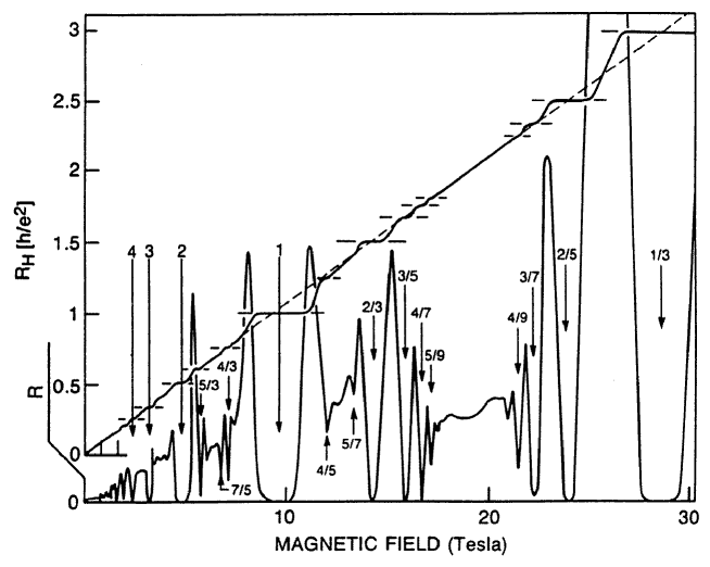
Figure 1.2: Integer and fractional quantum Hall transport data showing the plateau regions in the Hall resistance $R_{\rm H}$ and associated dips in the dissipative resistance $R$. The numbers indicate the Landau level filling factors at which various features occur. After ref. [15].

shows the remarkable transport data for a real device in the quantum Hall regime. Instead of a Hall resistivity which is simply a linear function of magnetic field, we see a series of so-called Hall plateaus in which $\rho_{xy}$ is a universal constant

$$\rho_{xy}=-\frac{1}{\nu}\frac{h}{e^{2}}$$ (1.14)

independent of all microscopic details (including the precise value of the magnetic field). Associated with each of these plateaus is a dramatic decrease in the dissipative resistivity $\rho_{xx}\longrightarrow 0$ which drops as much as 13 orders of magnitude in the plateau regions. Clearly the system is undergoing some sort of sequence of phase transitions into highly idealized dissipationless states. Just as in a superconductor, the dissipationless state supports persistent currents. These can be produced in devices having the Corbino ring geometry shown in fig. (1.3).

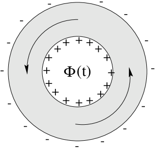
Figure 1.3: Persistent current circulating in a quantum Hall device having the Corbino geometry. The radial electric field is maintained by the charges which can not flow back together because $\sigma_{xx}$ is nearly zero. These charges result from the radial current pulse associated with the azimuthal electric field pulse produced by the applied flux $\Phi(t)$.

Applying additional flux through the ring produces a temporary azimuthal electric field by Faraday induction. A current pulse is induced at right angles to the $E$ field and produces a radial charge polarization as shown. This polarization induces a (quasi-) permanent radial electric field which in turn causes persistent azimuthal currents. Torque magnetometer measurements [16] have shown that the currents can persist $\sim 10^{3}~{}\mbox{secs}$ at very low temperatures. After this time the tiny $\sigma_{xx}$ gradually allows the radial charge polarization to dissipate. We can think of the azimuthal currents as gradually spiraling outwards due to the Hall angle (between current and electric field) being very slightly less than $90^{\circ}$ (by $\sim 10^{-13}$).

We have shown that the random impurity potential (and by implication Anderson localization) is a necessary condition for Hall plateaus to occur, but we have not yet understood precisely how this novel behavior comes about. That is our next task.

1.2 Classical and Semi-Classical Dynamics

1.2.1 Classical Approximation

The classical equations of motion for an electron of charge $-e$ moving in two dimensions under the influence of the Lorentz force $\frac{-e}{c}\vec{v}\times\vec{B}$ caused by a magnetic field $\vec{B}=B\hat{z}$ are

$$m\ddot{x} = -\frac{eB}{c}\dot{y}$$ (1.15)

$$m\ddot{y} = +\frac{eB}{c}\dot{x}.$$ (1.16)

The general solution of these equations corresponds to motion in a circle of arbitrary radius $R$

$$\vec{r}=R\left(\cos(\omega_{c}t+\delta),\sin(\omega_{c}t+\delta)\right).$$ (1.17)

Here $\delta$ is an arbitrary phase for the motion and

$$\omega_{c}\equiv\frac{eB}{mc}$$ (1.18)

is known as the classical cyclotron frequency. Notice that the period of the orbit is independent of the radius and that the tangential speed

$$v=R\omega_{c}$$ (1.19)

controls the radius. A fast particle travels in a large circle but returns to the starting point in the same length of time as a slow particle which (necessarily) travels in a small circle. The motion is thus isochronous much like that of a harmonic oscillator whose period is independent of the amplitude of the motion. This apparent analogy is not an accident as we shall see when we study the Hamiltonian (which we will need for the full quantum solution).

Because of some subtleties involving distinctions between canonical and mechanical momentum in the presence of a magnetic field, it is worth reviewing the formal Lagrangian and Hamiltonian approaches to this problem. The above classical equations of motion follow from the Lagrangian

$$\mathcal{L}=\frac{1}{2}m\dot{x}^{\mu}\dot{x}^{\mu}-\frac{e}{c}\dot{x}^{\mu}A^{\mu},$$ (1.20)

where $\mu=1,2$ refers to $x$ and $y$ respectively and $\vec{A}$ is the vector potential evaluated at the position of the particle. (We use the Einstein summation convention throughout this discussion.) Using

$$\frac{\delta\mathcal{L}}{\delta x^{\nu}}=-\frac{e}{c}\dot{x}^{\mu}\,\partial_{\nu}A^{\mu}$$ (1.21)

and

$$\frac{\delta\mathcal{L}}{\delta\dot{x}^{\nu}}=m\dot{x}^{\nu}-\frac{e}{c}A^{\nu}$$ (1.22)

the Euler-Lagrange equation of motion becomes

$$m\ddot{x}^{\nu}=-\frac{e}{c}\left[\partial_{\nu}A^{\mu}-\partial_{\mu}A^{\nu}\right]\dot{x}^{\mu}.$$ (1.23)

Using

$$\vec{B} = \vec{\nabla}\times\vec{A}$$ (1.24)

$$B^{\alpha} = \epsilon^{\alpha\beta\gamma}\partial_{\beta}A^{\gamma}$$ (1.25)

shows that this is equivalent to eqs. (1.15–1.16).

Once we have the Lagrangian we can deduce the canonical momentum

$$p^{\mu} \equiv \frac{\delta\mathcal{L}}{\delta\dot{x}^{\mu}}$$ (1.26)

$$= m\dot{x}^{\mu}-\frac{e}{c}A^{\mu},$$

and the Hamiltonian

$$H[\vec{p},\vec{x}] \equiv \dot{x}^{\mu}p^{\mu}-\mathcal{L}(\dot{\vec{x}},\vec{x})$$ (1.27)

$$= \frac{1}{2m}\left(p^{\mu}+\frac{e}{c}A^{\mu}\right)\left(p^{\mu}+\frac{e}{c}A^{\mu}\right).$$

(Recall that the Lagrangian is canonically a function of the positions and velocities while the Hamiltonian is canonically a function of the positions and momenta). The quantity

$$p_{\mathrm{mech}}^{\mu}\equiv p^{\mu}+\frac{e}{c}A^{\mu}$$ (1.28)

is known as the mechanical momentum. Hamilton’s equations of motion

$$\dot{x}^{\mu} = \frac{\partial H}{\partial p^{\mu}}=\frac{1}{m}p_{\mathrm{mech}}^{\mu}$$ (1.29)

$$\dot{p}^{\mu} = -\frac{\partial H}{\partial x^{\mu}}=-\frac{e}{mc}\left(p^{\nu}+\frac{e}{c}A^{\nu}\right)\partial_{\mu}A^{\nu}$$ (1.30)

show that it is the mechanical momentum, not the canonical momentum, which is equal to the usual expression related to the velocity

$$p_{\mathrm{mech}}^{\mu}=m\dot{x}^{\mu}.$$ (1.31)

Using Hamilton’s equations of motion we can recover Newton’s law for the Lorentz force given in eq. (1.23) by simply taking a time derivative of $\dot{x}^{\mu}$ in eq. (1.29) and then using eq. (1.30).

The distinction between canonical and mechanical momentum can lead to confusion. For example it is possible for the particle to have a finite velocity while having zero (canonical) momentum! Furthermore the canonical momentum is dependent (as we will see later) on the choice of gauge for the vector potential and hence is not a physical observable. The mechanical momentum, being simply related to the velocity (and hence the current) is physically observable and gauge invariant. The classical equations of motion only involve the curl of the vector potential and so the particular gauge choice is not very important at the classical level. We will therefore delay discussion of gauge choices until we study the full quantum solution, where the issue is unavoidable.

1.2.2 Semi-classical Approximation

Recall that in the semi-classical approximation used in transport theory we consider wave packets $\Psi_{\vec{R}(t),\vec{K}(t)}(\vec{r},t)$ made up of a linear superposition of Bloch waves. These packets are large on the scale of the de Broglie wavelength so that they have a well-defined central wave vector $\vec{K}(t)$, but they are small on the scale of everything else (external potentials, etc.) so that they simultaneously can be considered to have well-defined mean position $R(t)$. (Note that $\vec{K}$ and $\vec{R}$ are parameters labeling the wave packet not arguments.) We then argue (and will discuss further below) that the solution of the Schrödinger equation in this semiclassical limit gives a wave packet whose parameters $\vec{K}(t)$ and $\vec{R}(t)$ obey the appropriate analog of the classical Hamilton equations of motion

$$\dot{R}^{\mu} = \frac{\partial\langle\Psi_{\vec{R},\vec{K}}|H|\Psi_{\vec{R},\vec{K}}\rangle}{\partial\hbar K^{\mu}}$$ (1.32)

$$\hbar\dot{K}^{\mu} = -\frac{\partial\langle\Psi_{\vec{R},\vec{K}}|H|\Psi_{\vec{R},\vec{K}}\rangle}{\partial R^{\mu}}.$$ (1.33)

Naturally this leads to the same circular motion of the wave packet at the classical cyclotron frequency discussed above. For weak fields and fast electrons the radius of these circular orbits will be large compared to the size of the wave packets and the semi-classical approximation will be valid. However at strong fields, the approximation begins to break down because the orbits are too small and because $\hbar\omega_{c}$ becomes a significant (large) energy. Thus we anticipate that the semi-classical regime requires $\hbar\omega_{c}\ll\epsilon_{\mathrm{F}}$, where $\epsilon_{\mathrm{F}}$ is the Fermi energy.

We have already seen hints that the problem we are studying is really a harmonic oscillator problem. For the harmonic oscillator there is a characteristic energy scale $\hbar\omega$ (in this case $\hbar\omega_{c}$) and a characteristic length scale $\ell$ for the zero-point fluctuations of the position in the ground state. The analog quantity in this problem is the so-called magnetic length

$$\ell\equiv\sqrt{\frac{\hbar c}{eB}}=\frac{257\hbox{\AA}}{\sqrt{\frac{B}{1\mathrm{tesla}}}}.$$ (1.34)

The physical interpretation of this length is that the area $2\pi\ell^{2}$ contains one quantum of magnetic flux $\Phi_{0}$ where

$$\Phi_{0}=\frac{hc}{e}.$$ (1.35)

That is to say, the density of magnetic flux is

$$B=\frac{\Phi_{0}}{2\pi\ell^{2}}.$$ (1.36)

To be in the semiclassical limit then requires that the Fermi wavelength be small on the scale of the magnetic length so that $k_{\mathrm{F}}\ell\gg 1$. This condition turns out to be equivalent to $\hbar\omega_{c}\ll\epsilon_{\mathrm{F}}$ so they are not separate constraints.

Exercise 1.1

Use the Bohr-Sommerfeld quantization condition that the orbit have a circumference containing an integral number of de Broglie wavelengths to find the allowed orbits of a 2D electron moving in a uniform magnetic field. Show that each successive orbit encloses precisely one additional quantum of flux in its interior. Hint: It is important to make the distinction between the canonical momentum (which controls the de Broglie wavelength) and the mechanical momentum (which controls the velocity). The calculation is simplified if one uses the symmetric gauge $\vec{A}=-\frac{1}{2}\vec{r}\times\vec{B}$ in which the vector potential is purely azimuthal and independent of the azimuthal angle.

1.3 Quantum Dynamics in Strong B Fields

Since we will be dealing with the Hamiltonian and the Schrödinger equation, our first order of business is to choose a gauge for the vector potential. One convenient choice is the so-called Landau gauge:

$$\vec{A}(\vec{r}\,)=xB\hat{y}$$ (1.37)

which obeys $\vec{\nabla}\times\vec{A}=B\hat{z}$. In this gauge the vector potential points in the $y$ direction but varies only with the $x$ position, as illustrated in fig. (1.4).

Figure 1.4: Illustration of the Landau gauge vector potential $\vec{A}=xB\hat{y}$. The magnetic field is perfectly uniform, but the vector potential has a preferred origin and orientation corresponding to the particular gauge choice.

Hence the system still has translation invariance in the $y$ direction. Notice that the magnetic field (and hence all the physics) is translationally invariant, but the Hamiltonian is not! (See exercise 1.2.) This is one of many peculiarities of dealing with vector potentials.

Exercise 1.2

Show for the Landau gauge that even though the Hamiltonian is not invariant for translations in the $x$ direction, the physics is still invariant since the change in the Hamiltonian that occurs under translation is simply equivalent to a gauge change. Prove this for any arbitrary gauge, assuming only that the magnetic field is uniform.

The Hamiltonian can be written in the Landau gauge as

$$H=\frac{1}{2m}\left(p_{x}^{2}+(p_{y}+\frac{eB}{c}x)^{2}\right)$$ (1.38)

Taking advantage of the translation symmetry in the $y$ direction, let us attempt a separation of variables by writing the wave function in the form

$$\psi_{k}(x,y)=e^{iky}f_{k}(x).$$ (1.39)

This has the advantage that it is an eigenstate of $p_{y}$ and hence we can make the replacement $p_{y}\longrightarrow\hbar k$ in the Hamiltonian. After separating variables we have the effective one-dimensional Schrödinger equation

$$h_{k}f_{k}(x)=\epsilon_{k}f_{k}(x),$$ (1.40)

where

$$h_{k}\equiv\frac{1}{2m}p_{x}^{2}+\frac{1}{2m}\left(\hbar k+\frac{eB}{c}x\right)^{2}.$$ (1.41)

This is simply a one-dimensional displaced harmonic oscillator

$$h_{k}=\frac{1}{2m}p_{x}^{2}+\frac{1}{2}m\omega_{c}^{2}\left(x+k\ell^{2}\right)^{2}$$ (1.42)

whose frequency is the classical cyclotron frequency and whose central position $X_{k}=-k\ell^{2}$ is (somewhat paradoxically) determined by the $y$ momentum quantum number. Thus for each plane wave chosen for the $y$ direction there will be an entire family of energy eigenvalues

$$\epsilon_{kn}=(n+\frac{1}{2})\hbar\omega_{c}$$ (1.43)

which depend only on $n$ are completely independent of the $y$ momentum $\hbar k$. The corresponding (unnormalized) eigenfunctions are

$$\psi_{nk}(\vec{r}\,)=\frac{1}{\sqrt{L}}e^{iky}H_{n}(x+k\ell^{2})e^{-\frac{1}{2\ell^{2}}(x+k\ell^{2})^{2}},$$ (1.44)

where $H_{n}$ is (as usual for harmonic oscillators) the $n$th Hermite polynomial (in this case displaced to the new central position $X_{k}$).

Exercise 1.3

Verify that eq. (1.44) is in fact a solution of the Schrödinger equation as claimed.

These harmonic oscillator levels are called Landau levels. Due to the lack of dependence of the energy on $k$, the degeneracy of each level is enormous, as we will now show. We assume periodic boundary conditions in the $y$ direction. Because of the vector potential, it is impossible to simultaneously have periodic boundary conditions in the $x$ direction. However since the basis wave functions are harmonic oscillator polynomials multiplied by strongly converging gaussians, they rapidly vanish for positions away from the center position $X_{0}=-k\ell^{2}$. Let us suppose that the sample is rectangular with dimensions $L_{x},L_{y}$ and that the left hand edge is at $x=-L_{x}$ and the right hand edge is at $x=0$. Then the values of the wavevector $k$ for which the basis state is substantially inside the sample run from $k=0$ to $k=L_{x}/\ell^{2}$. It is clear that the states at the left edge and the right edge differ strongly in their $k$ values and hence periodic boundary conditions are impossible.

The total number of states in each Landau level is then

$$N=\frac{L_{y}}{2\pi}\int_{0}^{L_{x}/\ell^{2}}dk=\frac{L_{x}L_{y}}{2\pi\ell^{2}}=N_{\Phi}$$ (1.45)

where

$$N_{\Phi}\equiv\frac{BL_{x}L_{y}}{\Phi_{0}}$$ (1.46)

is the number of flux quanta penetrating the sample. Thus there is one state per Landau level per flux quantum which is consistent with the semiclassical result from Exercise (1.1). Notice that even though the family of allowed wavevectors is only one-dimensional, we find that the degeneracy of each Landau level is extensive in the two-dimensional area. The reason for this is that the spacing between wave vectors allowed by the periodic boundary conditions $\Delta_{k}=\frac{2\pi}{L_{y}}$ decreases while the range of allowed wave vectors $[0,L_{x}/\ell^{2}]$ increases with increasing $L$. The reader may also worry that for very large samples, the range of allowed values of $k$ will be so large that it will fall outside the first Brillouin zone forcing us to include band mixing and the periodic lattice potential beyond the effective mass approximation. This is not true however, since the canonical momentum is a gauge dependent quantity. The value of $k$ in any particular region of the sample can be made small by shifting the origin of the coordinate system to that region (thereby making a gauge transformation).

The width of the harmonic oscillator wave functions in the $n$th Landau level is of order $\sqrt{n}\ell$. This is microscopic compared to the system size, but note that the spacing between the centers

$$\Delta=\Delta_{k}\ell^{2}=\frac{2\pi\ell^{2}}{L_{y}}$$ (1.47)

is vastly smaller (assuming $L_{y}>>\ell$). Thus the supports of the different basis states are strongly overlapping (but they are still orthogonal).

Exercise 1.4

Using the fact that the energy for the $n$th harmonic oscillator state is $(n+\frac{1}{2})\hbar\omega_{c}$, present a semi-classical argument explaining the result claimed above that the width of the support of the wave function scales as $\sqrt{n}\ell$.

Exercise 1.5

Using the Landau gauge, construct a gaussian wave packet in the lowest Landau level of the form $$\Psi(x,y)=\int_{-\infty}^{+\infty}a_{k}e^{iky}e^{-\frac{1}{2\ell^{2}}(x+k\ell^{2})^{2}},$$ choosing $a_{k}$ in such a way that the wave packet is localized as closely as possible around some point $\vec{R}$. What is the smallest size wave packet that can be constructed without mixing in higher Landau levels?

Having now found the eigenfunctions for an electron in a strong magnetic field we can relate them back to the semi-classical picture of wave packets undergoing circular cyclotron motion. Consider an initial semiclassical wave packet located at some position and having some specified momentum. In the semiclassical limit the mean energy of this packet will greatly exceed the cyclotron energy $\frac{\hbar^{2}K^{2}}{2m}\gg\hbar\omega_{c}$ and hence it will be made up of a linear combination of a large number of different Landau level states centered around $\bar{n}=\frac{\hbar^{2}K^{2}}{2m\hbar\omega_{c}}$

$$\Psi(\vec{r},t)=\sum_{n}\int L_{y}\frac{dk}{2\pi}\,a_{n}(\vec{k})\psi_{nk}(\vec{r}\,)e^{-i(n+\frac{1}{2})\omega_{c}t}.$$ (1.48)

Notice that in an ordinary 2D problem at zero field, the complete set of plane wave states would be labeled by a 2D continuous momentum label. Here we have one discrete label (the Landau level index) and a 1D continuous labels (the $y$ wave vector). Thus the ‘sum’ over the complete set of states is actually a combination of a summation and an integration.

The details of the initial position and momentum are controlled by the amplitudes $a_{n}(\vec{k})$. We can immediately see however, that since the energy levels are exactly evenly spaced that the motion is exactly periodic:

$$\Psi(\vec{r},t+\frac{2\pi}{\omega_{c}})=\Psi(\vec{r},t).$$ (1.49)

If one works through the details, one finds that the motion is indeed circular and corresponds to the expected semi-classical cyclotron orbit.

For simplicity we will restrict the remainder of our discussion to the lowest Landau level where the (correctly normalized) eigenfunctions in the Landau gauge are (dropping the index $n=0$ from now on):

$$\psi_{k}(\vec{r}\,)=\frac{1}{\sqrt{\pi^{1/2}L\ell}}e^{iky}e^{-\frac{1}{2\ell^{2}}(x+k\ell^{2})^{2}}$$ (1.50)

and every state has the same energy eigenvalue $\epsilon_{k}=\frac{1}{2}\hbar\omega_{c}$.

We imagine that the magnetic field (and hence the Landau level splitting) is very large so that we can ignore higher Landau levels. (There are some subtleties here to which we will return.) Because the states are all degenerate, any wave packet made up of any combination of the basis states will be a stationary state. The total current will therefore be zero. We anticipate however from semiclassical considerations that there should be some remnant of the classical circular motion visible in the local current density. To see this note that the expectation value of the current in the $k$th basis state is

$$\langle\vec{J}\,\rangle=-e\frac{1}{m}\left\langle\Psi_{k}\left|\left(\vec{p}+\frac{e}{c}\vec{A}\,\right)\right|\Psi_{k}\right\rangle.$$ (1.51)

The $y$ component of the current is

$$\langle J_{y}\rangle = -\frac{e}{m\pi^{1/2}\ell}\int dx\,e^{-\frac{1}{2\ell^{2}}(x+k\ell^{2})^{2}}\left(\hbar k+\frac{eB}{c}x\right)e^{-\frac{1}{2\ell^{2}}(x+k\ell^{2})^{2}}$$ (1.52)

$$= -\frac{e\omega_{c}}{\pi^{1/2}\ell}\int dx\,e^{-\frac{1}{\ell^{2}}(x+k\ell^{2})^{2}}\left(x+k\ell^{2}\right)$$

We see from the integrand that the current density is antisymmetric about the peak of the gaussian and hence the total current vanishes. This antisymmetry (positive vertical current on the left, negative vertical current on the right) is the remnant of the semiclassical circular motion.

Let us now consider the case of a uniform electric field pointing in the $x$ direction and giving rise to the potential energy

$$V(\vec{r}\,)=+eEx.$$ (1.53)

This still has translation symmetry in the $y$ direction and so our Landau gauge choice is still the most convenient. Again separating variables we see that the solution is nearly the same as before, except that the displacement of the harmonic oscillator is slightly different. The Hamiltonian in eq. (1.54) becomes

$$h_{k}=\frac{1}{2m}p_{x}^{2}+\frac{1}{2}m\omega_{c}^{2}\left(x+k\ell^{2}\right)^{2}+eEx.$$ (1.54)

Completing the square we see that the oscillator is now centered at the new position

$$X_{k}=-k\ell^{2}-\frac{eE}{m\omega_{c}^{2}}$$ (1.55)

and the energy eigenvalue is now linearly dependent on the particle’s peak position $X_{k}$ (and therefore linear in the $y$ momentum)

$$\epsilon_{k}=\frac{1}{2}\hbar\omega_{c}+eEX_{k}+\frac{1}{2}m\bar{v}^{2},$$ (1.56)

where

$$\bar{v}\equiv-c\frac{E}{B}.$$ (1.57)

Because of the shift in the peak position of the wavefunction, the perfect antisymmetry of the current distribution is destroyed and there is a net current

$$\langle J_{y}\rangle=-e\bar{v}$$ (1.58)

showing that $\bar{v}\hat{y}$ is simply the usual $c\vec{E}\times\vec{B}/B^{2}$ drift velocity. This result can be derived either by explicitly doing the integral for the current or by noting that the wave packet group velocity is

$$\frac{1}{\hbar}\frac{\partial\epsilon_{k}}{\partial k}=\frac{eE}{\hbar}\frac{\partial X_{k}}{\partial k}=\bar{v}$$ (1.59)

independent of the value of $k$ (since the electric field is a constant in this case, giving rise to a strictly linear potential). Thus we have recovered the correct kinematics from our quantum solution.

It should be noted that the applied electric field ‘tilts’ the Landau levels in the sense that their energy is now linear in position as illustrated in fig.(1.5).

Figure 1.5: Illustration of electron Landau energy levels $\left(n+\frac{1}{2}\right)\hbar\omega_{\mathrm{c}}$ vs. position $x_{k}=-k\ell^{2}$. (a) Zero electric field case. (b) Case with finite electric field pointing in the $+\hat{x}$ direction.

This means that there are degeneracies between different Landau level states because different kinetic energy can compensate different potential energy in the electric field. Nevertheless, we have found the exact eigenstates (i.e., the stationary states). It is not possible for an electron to decay into one of the other degenerate states because they have different canonical momenta. If however disorder or phonons are available to break translation symmetry, then these decays become allowed and dissipation can appear. The matrix elements for such processes are small if the electric field is weak because the degenerate states are widely separated spatially due to the small tilt of the Landau levels.

Exercise 1.6

It is interesting to note that the exact eigenstates in the presence of the electric field can be viewed as displaced oscillator states in the original (zero $E$ field) basis. In this basis the displaced states are linear combinations of all the Landau level excited states of the same $k$. Use first-order perturbation theory to find the amount by which the $n=1$ Landau level is mixed into the $n=0$ state. Compare this with the exact amount of mixing computed using the exact displaced oscillator state. Show that the two results agree to first order in $E$. Because the displaced state is a linear combination of more than one Landau level, it can carry a finite current. Give an argument, based on perturbation theory why the amount of this current is inversely proportional to the $B$ field, but is independent of the mass of the particle. Hint: how does the mass affect the Landau level energy spacing and the current operator?

1.4 IQHE Edge States

Now that we understand drift in a uniform electric field, we can consider the problem of electrons confined in a Hall bar of finite width by a non-uniform electric field. For simplicity, we will consider the situation where the potential $V(x)$ is smooth on the scale of the magnetic length, but this is not central to the discussion. If we assume that the system still has translation symmetry in the $y$ direction, the solution to the Schrödinger equation must still be of the form

$$\psi(x,y)=\frac{1}{\sqrt{L_{y}}}e^{iky}f_{k}(x).$$ (1.60)

The function $f_{k}$ will no longer be a simple harmonic wave function as we found in the case of the uniform electric field. However we can anticipate that $f_{k}$ will still be peaked near (but in general not precisely at) the point $X_{k}\equiv-k\ell^{2}$. The eigenvalues $\epsilon_{k}$ will no longer be precisely linear in $k$ but will still reflect the kinetic energy of the cyclotron motion plus the local potential energy $V(X_{k})$ (plus small corrections analogous to the one in eq. (1.56)). This is illustrated in fig. (1.6).

Figure 1.6: Illustration of a smooth confining potential which varies only in the $x$ direction. The horizontal dashed line indicates the equilibrium fermi level. The dashed curve indicates the wave packet envelope $f_{k}$ which is displaced from its nominal position $x_{k}\equiv-k\ell^{2}$ by the slope of the potential.

We see that the group velocity

$$\vec{v}_{k}=\frac{1}{\hbar}\frac{\partial\epsilon_{k}}{\partial k}\hat{y}$$ (1.61)

has the opposite sign on the two edges of the sample. This means that in the ground state there are edge currents of opposite sign flowing in the sample. The semi-classical interpretation of these currents is that they represent ‘skipping orbits’ in which the circular cyclotron motion is interrupted by collisions with the walls at the edges as illustrated in fig. (1.7).

Figure 1.7: Semi-classical view of skipping orbits at the fermi level at the two edges of the sample where the confining electric field causes $\vec{E}\times\vec{B}$ drift. The circular orbit illustrated in the center of the sample carries no net drift current if the local electric field is zero.

One way to analyze the Hall effect in this system is quite analogous to the Landauer picture of transport in narrow wires [17, 18]. The edge states play the role of the left and right moving states at the two fermi points. Because (as we saw earlier) momentum in a magnetic field corresponds to position, the edge states are essentially real space realizations of the fermi surface. A Hall voltage drop across the sample in the $x$ direction corresponds to a difference in electrochemical potential between the two edges. Borrowing from the Landauer formulation of transport, we will choose to apply this in the form of a chemical potential difference and ignore any changes in electrostatic potential. What this does is increase the number of electrons in skipping orbits on one edge of the sample and/or decrease the number on the other edge. Previously the net current due to the two edges was zero, but now there is a net Hall current. To calculate this current we have to add up the group velocities of all the occupied states

$$I=-\frac{e}{L_{y}}\int_{-\infty}^{+\infty}dk\frac{L_{y}}{2\pi}\,\frac{1}{\hbar}\frac{\partial\epsilon_{k}}{\partial k}n_{k},$$ (1.62)

where for the moment we assume that in the bulk, only a single Landau level is occupied and $n_{k}$ is the probability that state $k$ in that Landau level is occupied. Assuming zero temperature and noting that the integrand is a perfect derivative, we have

$$I=-\frac{e}{h}\int_{\mu_{R}}^{\mu_{L}}d\epsilon=-\frac{e}{h}\left[\mu_{L}-\mu_{R}\right].$$ (1.63)

(To understand the order of limits of integration, recall that as $k$ increases, $X_{k}$ decreases.) The definition of the Hall voltage drop is

$$(+e)V_{H}\equiv(+e)\left[V_{R}-V_{L}\right]=\left[\mu_{R}-\mu_{L}\right].$$ (1.64)

Hence

$$I=-\nu\frac{e^{2}}{h}V_{H},$$ (1.65)

where we have now allowed for the possibility that $\nu$ different Landau levels are occupied in the bulk and hence there are $\nu$ separate edge channels contributing to the current. This is the analog of having $\nu$ ‘open’ channels in the Landauer transport picture. In the Landauer picture for an ordinary wire, we are considering the longitudinal voltage drop (and computing $\sigma_{xx}$), while here we have the Hall voltage drop (and are computing $\sigma_{xy}$). The analogy is quite precise however because we view the right and left movers as having distributions controlled by separate chemical potentials. It just happens in the QHE case that the right and left movers are physically separated in such a way that the voltage drop is transverse to the current. Using the above result and the fact that the current flows at right angles to the voltage drop we have the desired results

$$\sigma_{xx} = 0$$ (1.66)

$$\sigma_{xy} = -\nu\frac{e^{2}}{h},$$ (1.67)

with the quantum number $\nu$ being an integer.

So far we have been ignoring the possible effects of disorder. Recall that for a single-channel one-dimensional wire in the Landauer picture, a disordered region in the middle of the wire will reduce the conductivity to

$$I=\frac{e^{2}}{h}|T|^{2},$$ (1.68)

where $|T|^{2}$ is the probability for an electron to be transmitted through the disordered region. The reduction in transmitted current is due to back scattering. Remarkably, in the QHE case, the back scattering is essentially zero in very wide samples. To see this note that in the case of the Hall bar, scattering into a backward moving state would require transfer of the electron from one edge of the sample to the other since the edge states are spatially separated. For samples which are very wide compared to the magnetic length (more precisely, to the Anderson localization length) the matrix element for this is exponentially small. In short, there can be nothing but forward scattering. An incoming wave given by eq. (1.60) can only be transmitted in the forward direction, at most suffering a simple phase shift $\delta_{k}$

$$\psi_{\mathrm{out}}(x,y)=\frac{1}{\sqrt{L_{y}}}e^{i\delta_{k}}e^{iky}f_{k}(x).$$ (1.69)

This is because no other states of the same energy are available. If the disorder causes Landau level mixing at the edges to occur (because the confining potential is relatively steep) then it is possible for an electron in one edge channel to scatter into another, but the current is still going in the same direction so that there is no reduction in overall transmission probability. It is this chiral (unidirectional) nature of the edge states which is responsible for the fact that the Hall conductance is correctly quantized independent of the disorder.

Disorder will broaden the Landau levels in the bulk and provide a reservoir of (localized) states which will allow the chemical potential to vary smoothly with density. These localized states will not contribute to the transport and so the Hall conductance will be quantized over a plateau of finite width in $B$ (or density) as seen in the data. Thus obtaining the universal value of quantized Hall conductance to a precision of $10^{-10}$ does not require fine tuning the applied $B$ field to a similar precision.

The localization of states in the bulk by disorder is an essential part of the physics of the quantum Hall effect as we saw when we studied the role of translation invariance. We learned previously that in zero magnetic field all states are (weakly) localized in two dimensions. In the presence of a quantizing magnetic field, most states are strongly localized as discussed above. However if all states were localized then it would be impossible to have a quantum phase transition from one QHE plateau to the next. To understand how this works it is convenient to work in a semiclassical percolation picture to be described below.

Exercise 1.7

Show that the number of edge channels whose energies lie in the gap between two Landau levels scales with the length $L$ of the sample, while the number of bulk states scales with the area. Use these facts to show that the range of magnetic field in which the chemical potential lies in between two Landau levels scales to zero in the thermodynamic limit. Hence finite width quantized Hall plateaus can not occur in the absence of disorder that produces a reservoir of localized states in the bulk whose number is proportional to the area.

1.5 Semiclassical Percolation Picture

Let us consider a smooth random potential caused, say, by ionized silicon donors remotely located away from the 2DEG in the GaAs semiconductor host. We take the magnetic field to be very large so that the magnetic length is small on the scale over which the potential varies. In addition, we ignore the Coulomb interactions among the electrons.

What is the nature of the eigenfunctions in this random potential? We have learned how to solve the problem exactly for the case of a constant electric field and know the general form of the solution when there is translation invariance in one direction. We found that the wave functions were plane waves running along lines of constant potential energy and having a width perpendicular to this which is very small and on the order of the magnetic length. The reason for this is the discreteness of the kinetic energy in a strong magnetic field. It is impossible for an electron stuck in a given Landau level to continuously vary its kinetic energy. Hence energy conservation restricts its motion to regions of constant potential energy. In the limit of infinite magnetic field where Landau level mixing is completely negligible, this confinement to lines of constant potential becomes exact (as the magnetic length goes to zero).

We are led to the following somewhat paradoxical picture. The strong magnetic field should be viewed as putting the system in the quantum limit in the sense that $\hbar\omega_{c}$ is a very large energy (comparable to $\epsilon_{\mathrm{F}}$). At the same time (if one assumes the potential is smooth) one can argue that since the magnetic length is small compared to the scale over which the random potential varies, the system is in a semi-classical limit where small wave packets (on the scale of $\ell$) follow classical $\vec{E}\times\vec{B}$ drift trajectories.

From this discussion it then seems very reasonable that in the presence of a smooth random potential, with no particular translation symmetry, the eigenfunctions will live on contour lines of constant energy on the random energy surface. Thus low energy states will be found lying along contours in deep valleys in the potential landscape while high energy states will be found encircling ‘mountain tops’ in the landscape. Naturally these extreme states will be strongly localized about these extrema in the potential.

Exercise 1.8

Using the Lagrangian for a charged particle in a magnetic field with a scalar potential $V(\vec{r}\,)$, consider the high field limit by setting the mass to zero (thereby sending the quantum cyclotron energy to infinity). 1. Derive the classical equations of motion from the Lagrangian and show that they yield simple $\vec{E}\times\vec{B}$ drift along isopotential contours. 2. Find the momentum conjugate to the coordinate $x$ and show that (with an appropriate gauge choice) it is the coordinate $y$: $$p_{x}=-\frac{\hbar}{\ell^{2}}y$$ (1.70) so that we have the strange commutation relation $$[x,y]=-i\ell^{2}.$$ (1.71) In the infinite field limit where $\ell\rightarrow 0$ the coordinates commute and we recover the semi-classical result in which effectively point particles drift along isopotentials.

To understand the nature of states at intermediate energies, it is useful to imagine gradually filling a random landscape with water as illustrated in fig. (1.8).

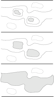
Figure 1.8: Contour map of a smooth random landscape. Closed dashed lines indicate local mountain peaks. Closed solid lines indicate valleys. From top to bottom, the gray filled areas indicate the increasing ‘sea level’ whose shoreline finally percolates from one edge of the sample to the other (bottom panel). The particle-hole excitations live along the shoreline and become gapless when the shoreline becomes infinite in extent.

In this analogy, sea level represents the chemical potential for the electrons. When only a small amount of water has been added, the water will fill the deepest valleys and form small lakes. As the sea level is increased the lakes will grow larger and their shorelines will begin to take on more complex shapes. At a certain critical value of sea level a phase transition will occur in which the shoreline percolates from one side of the system to the other. As the sea level is raised still further, the ocean will cover the majority of the land and only a few mountain tops will stick out above the water. The shore line will no longer percolate but only surround the mountain tops.

As the sea level is raised still higher additional percolation transitions will occur successively as each successive Landau level passes under water. If Landau level mixing is small and the disorder potential is symmetrically distributed about zero, then the critical value of the chemical potential for the $n$th percolation transition will occur near the center of the $n$th Landau level

$$\mu^{*}_{n}=(n+\frac{1}{2})\hbar\omega_{c}.$$ (1.72)

This percolation transition corresponds to the transition between quantized Hall plateaus. To see why, note that when the sea level is below the percolation point, most of the sample is dry land. The electron gas is therefore insulating. When sea level is above the percolation point, most of the sample is covered with water. The electron gas is therefore connected throughout the majority of the sample and a quantized Hall current can be carried. Another way to see this is to note that when the sea level is above the percolation point, the confining potential will make a shoreline along the full length of each edge of the sample. The edge states will then carry current from one end of the sample to the other.

We can also understand from this picture why the dissipative conductivity $\sigma_{xx}$ has a sharp peak just as the plateau transition occurs. (Recall the data in fig. (1.2).) Away from the critical point the circumference of any particular patch of shoreline is finite. The period of the semiclassical orbit around this is finite and hence so is the quantum level spacing. Thus there are small energy gaps for excitation of states across these real-space fermi levels. Adding an infinitesimal electric field will only weakly perturb these states due to the gap and the finiteness of the perturbing matrix element which will be limited to values on the order of $\sim eED$ where $D$ is the diameter of the orbit. If however the shoreline percolates from one end of the sample to the other then the orbital period diverges and the gap vanishes. An infinitesimal electric field can then cause dissipation of energy.

Another way to see this is that as the percolation level is approached from above, the edge states on the two sides will begin taking detours deeper and deeper into the bulk and begin communicating with each other as the localization length diverges and the shoreline zig zags throughout the bulk of the sample. Thus electrons in one edge state can be back scattered into the other edge states and ultimately reflected from the sample as illustrated in fig. (1.9).

Figure 1.9: Illustration of edge states that wander deep into the bulk as the quantum Hall localization transition is approached from the conducting side. Solid arrows indicate the direction of drift along the isopotential lines. Dashed arrows indicate quantum tunneling from one semi-classical orbit (edge state) to the other. This backscattering localizes the eigenstates and prevents transmission through the sample using the ‘edge’ states (which become part of the bulk localized states).

Because the random potential broadens out the Landau level density of states, the quantized Hall plateaus will have finite width. As the chemical potential is varied in the regime of localized states in between the Landau level peaks, only the occupancy of localized states is changing. Hence the transport properties remain constant until the next percolation transition occurs. It is important to have the disorder present to produce this finite density of states and to localize those states.

It is known that as the (classical) percolation point is approached in two dimensions, the characteristic size (diameter) of the shoreline orbits diverges like

$$\xi\sim|\delta|^{-4/3},$$ (1.73)

where $\delta$ measures the deviation of the sea level from its critical value. The shoreline structure is not smooth and in fact its circumference diverges with a larger exponent $7/3$ showing that these are highly ramified fractal objects whose circumference scales as the $7/4$th power of the diameter.

So far we have assumed that the magnetic length is essentially zero. That is, we have ignored the fact that the wave function support extends a small distance transverse to the isopotential lines. If two different orbits with the same energy pass near each other but are classically disconnected, the particle can still tunnel between them if the magnetic length is finite. This quantum tunneling causes the localization length to diverge faster than the classical percolation model predicts. Numerical simulations find that the localization length diverges like [19, 20, 21, 22]

$$\xi\sim|\delta|^{-\nu}$$ (1.74)

where the exponent $\nu$ (not to be confused with the Landau level filling factor!) has a value close (but probably not exactly equal to) $7/3$ rather than the $4/3$ found in classical percolation. It is believed that this exponent is universal and independent of Landau level index.

Experiments on the quantum critical behavior are quite difficult but there is evidence [23], at least in selected samples which show good scaling, that $\nu$ is indeed close to $7/3$ (although there is some recent controversy on this point. [24]) and that the conductivity tensor is universal at the critical point. [21, 25] Why Coulomb interactions that are present in real samples do not spoil agreement with the numerical simulations is something of a mystery at the time of this writing. For a discussion of some of these issues see [13].

1.6 Fractional QHE

Under some circumstances of weak (but non-zero) disorder, quantized Hall plateaus appear which are characterized by simple rational fractional quantum numbers. For example, at magnetic fields three times larger than those at which the $\nu=1$ integer filling factor plateau occurs, the lowest Landau level is only 1/3 occupied. The system ought to be below the percolation threshold and hence be insulating. Instead a robust quantized Hall plateau is observed indicating that electrons can travel through the sample and that (since $\sigma_{xx}\longrightarrow 0$) there is an excitation gap. This novel and quite unexpected physics is controlled by Coulomb repulsion between the electrons. It is best understood by first ignoring the disorder and trying to discover the nature of the special correlated many-body ground state into which the electrons condense when the filling factor is a rational fraction.

For reasons that will become clear later, it is convenient to analyze the problem in a new gauge

$$\vec{A}=-\frac{1}{2}\vec{r}\times\vec{B}$$ (1.75)

known as the symmetric gauge. Unlike the Landau gauge which preserves translation symmetry in one direction, the symmetric gauge preserves rotational symmetry about the origin. Hence we anticipate that angular momentum (rather than $y$ linear momentum) will be a good quantum number in this gauge.

For simplicity we will restrict our attention to the lowest Landau level only and (simply to avoid some awkward minus signs) change the sign of the $B$ field: $\vec{B}=-B\hat{z}$. With these restrictions, it is not hard to show that the solutions of the free-particle Schrödinger equation having definite angular momentum are

$$\varphi_{m}=\frac{1}{\sqrt{2\pi\ell^{2}2^{m}m!}}z^{m}e^{-\frac{1}{4}|z|^{2}}$$ (1.76)

where $z=(x+iy)/\ell$ is a dimensionless complex number representing the position vector $\vec{r}\equiv(x,y)$ and $m\geq 0$ is an integer.

Exercise 1.9

Verify that the basis functions in eq. (1.76) do solve the Schrödinger equation in the absence of a potential and do lie in the lowest Landau level. Hint: Rewrite the kinetic energy in such a way that $\vec{p}\cdot\vec{A}$ becomes $\vec{B}\cdot\vec{L}$.

The angular momentum of these basis states is of course $\hbar m$. If we restrict our attention to the lowest Landau level, then there exists only one state with any given angular momentum and only non-negative values of $m$ are allowed. This ‘handedness’ is a result of the chirality built into the problem by the magnetic field.

It seems rather peculiar that in the Landau gauge we had a continuous one-dimensional family of basis states for this two-dimensional problem. Now we find that in a different gauge, we have a discrete one dimensional label for the basis states! Nevertheless, we still end up with the correct density of states per unit area. To see this note that the peak value of $|\varphi_{m}|^{2}$ occurs at a radius of $R_{\mathrm{peak}}=\sqrt{2m\ell^{2}}$. The area $2\pi\ell^{2}m$ of a circle of this radius contains $m$ flux quanta. Hence we obtain the standard result of one state per Landau level per quantum of flux penetrating the sample.

Because all the basis states are degenerate, any linear combination of them is also an allowed solution of the Schrödinger equation. Hence any function of the form [26]

$$\Psi(x,y)=f(z)e^{-\frac{1}{4}|z|^{2}}$$ (1.77)

is allowed so long as $f$ is analytic in its argument. In particular, arbitrary polynomials of any degree $N$

$$f(z)=\prod_{j=1}^{N}(z-Z_{j})$$ (1.78)

are allowed (at least in the thermodynamic limit) and are conveniently defined by the locations of their $N$ zeros $\{Z_{j};j=1,2,\dots,N\}$.

Another useful solution is the so-called coherent state which is a particular infinite order polynomial

$$f_{\lambda}(z)\equiv\frac{1}{\sqrt{2\pi\ell^{2}}}e^{\frac{1}{2}\lambda^{*}z}e^{-\frac{1}{4}\lambda^{*}\lambda}.$$ (1.79)

The wave function using this polynomial has the property that it is a narrow gaussian wave packet centered at the position defined by the complex number $\lambda$. Completing the square shows that the probability density is given by

$$|\Psi_{\lambda}|^{2}=|f_{\lambda}|^{2}e^{-\frac{1}{2}|z|^{2}}=\frac{1}{2\pi\ell^{2}}e^{-\frac{1}{2}|z-\lambda|^{2}}$$ (1.80)

This is the smallest wave packet that can be constructed from states within the lowest Landau level. The reader will find it instructive to compare this gaussian packet to the one constructed in the Landau gauge in exercise (1.5).

Because the kinetic energy is completely degenerate, the effect of Coulomb interactions among the particles is nontrivial. To develop a feel for the problem, let us begin by solving the two-body problem. Recall that the standard procedure is to take advantage of the rotational symmetry to write down a solution with the relative angular momentum of the particles being a good quantum number and then solve the Schrödinger equation for the radial part of the wave function. Here we find that the analyticity properties of the wave functions in the lowest Landau level greatly simplifies the situation. If we know the angular behavior of a wave function, analyticity uniquely defines the radial behavior. Thus for example for a single particle, knowing that the angular part of the wave function is $e^{im\theta}$, we know that the full wave function is guaranteed to uniquely be $r^{m}e^{im\theta}e^{-\frac{1}{4}|z|^{2}}=z^{m}e^{-\frac{1}{4}|z|^{2}}$.

Consider now the two body problem for particles with relative angular momentum $m$ and center of mass angular momentum $M$. The unique analytic wave function is (ignoring normalization factors)

$$\Psi_{mM}(z_{1},z_{2})=(z_{1}-z_{2})^{m}(z_{1}+z_{2})^{M}e^{-\frac{1}{4}(|z_{1}|^{2}+|z_{2}|^{2})}.$$ (1.81)

If $m$ and $M$ are non-negative integers, then the prefactor of the exponential is simply a polynomial in the two arguments and so is a state made up of linear combinations of the degenerate one-body basis states $\varphi_{m}$ given in eq. (1.76) and therefore lies in the lowest Landau level. Note that if the particles are spinless fermions then $m$ must be odd to give the correct exchange symmetry. Remarkably, this is the exact (neglecting Landau level mixing) solution for the Schrödinger equation for any central potential $V(|z_{1}-z_{2}|)$ acting between the two particles. We do not need to solve any radial equation because of the powerful restrictions due to analyticity. There is only one state in the (lowest Landau level) Hilbert space with relative angular momentum $m$ and center of mass angular momentum $M$. Hence (neglecting Landau level mixing) it is an exact eigenstate of any central potential. $\Psi_{mM}$ is the exact answer independent of the Hamiltonian!

The corresponding energy eigenvalue $v_{m}$ is independent of $M$ and is referred to as the $m$th Haldane pseudopotential

$$v_{m}=\frac{\left\langle mM|V|mM\right\rangle}{\left\langle mM|mM\right\rangle}.$$ (1.82)

The Haldane pseudopotentials for the repulsive Coulomb potential are shown in fig. (1.10).

Figure 1.10: The Haldane pseudopotential $V_{m}$ vs. relative angular momentum $m$ for two particles interacting via the Coulomb interaction. Units are ${e^{2}}/{\epsilon\ell}$, where $\epsilon$ is the dielectric constant of the host semiconductor and the finite thickness of the quantum well has been neglected.

These discrete energy eigenstates represent bound states of the repulsive potential. If there were no magnetic field present, a repulsive potential would of course have only a continuous spectrum with no discrete bound states. However in the presence of the magnetic field, there are effectively bound states because the kinetic energy has been quenched. Ordinarily two particles that have a lot of potential energy because of their repulsive interaction can fly apart converting that potential energy into kinetic energy. Here however (neglecting Landau level mixing) the particles all have fixed kinetic energy. Hence particles that are repelling each other are stuck and can not escape from each other. One can view this semi-classically as the two particles orbiting each other under the influence of $\vec{E}\times\vec{B}$ drift with the Lorentz force preventing them from flying apart. In the presence of an attractive potential the eigenvalues change sign, but of course the eigenfunctions remain exactly the same (since they are unique)!

The fact that a repulsive potential has a discrete spectrum for a pair of particles is (as we will shortly see) the central feature of the physics underlying the existence of an excitation gap in the fractional quantum Hall effect. One might hope that since we have found analyticity to uniquely determine the two-body eigenstates, we might be able to determine many-particle eigenstates exactly. The situation is complicated however by the fact that for three or more particles, the various relative angular momenta $L_{12},L_{13},L_{23}$, etc. do not all commute. Thus we can not write down general exact eigenstates. We will however be able to use the analyticity to great advantage and make exact statements for certain special cases.

Exercise 1.10

Express the exact lowest Landau level two-body eigenstate $$\Psi(z_{1},z_{2})=(z_{1}-z_{2})^{3}\;e^{-\frac{1}{4}\left\{|z_{1}|^{2}+|z_{2}|^{2}\right\}}$$ in terms of the basis of all possible two-body Slater determinants.

Exercise 1.11

Verify the claim that the Haldane pseudopotential $v_{m}$ is independent of the center of mass angular momentum $M$.

Exercise 1.12

Evaluate the Haldane pseudopotentials for the Coulomb potential $\frac{e^{2}}{\epsilon r}$. Express your answer in units of $\frac{e^{2}}{\epsilon\ell}$. For the specific case of $\epsilon=10$ and $B=10$T, express your answer in Kelvin.

Exercise 1.13

Take into account the finite thickness of the quantum well by assuming that the one-particle basis states have the form $$\psi_{m}(z,s)=\varphi_{m}(z)\Phi(s),$$ where $s$ is the coordinate in the direction normal to the quantum well. Write down (but do not evaluate) the formal expression for the Haldane pseudo-potentials in this case. Qualitatively describe the effect of finite thickness on the values of the different pseudopotentials for the case where the well thickness is approximately equal to the magnetic length.

1.6.1 The $\nu=1$ many-body state

So far we have found the one- and two-body states. Our next task is to write down the wave function for a fully filled Landau level. We need to find

$$\psi[z]=f[z]\;e^{-\frac{1}{4}\sum_{j}|z_{j}|^{2}}$$ (1.83)

where $[z]$ stands for $(z_{1},z_{2},\ldots,z_{N})$ and $f$ is a polynomial representing the Slater determinant with all states occupied. Consider the simple example of two particles. We want one particle in the orbital $\varphi_{0}$ and one in $\varphi_{1}$, as illustrated schematically in fig. (1.11a).

Figure 1.11: Orbital occupancies for the maximal density filled Landau level state with (a) two particles and (b) three particles. There are no particle labels here. In the Slater determinant wave function, the particles are labeled but a sum is taken over all possible permutations of the labels in order to antisymmetrize the wave function.

Thus (again ignoring normalization)

$$f[z] = \left|\begin{array}[]{cc}(z_{1})^{0}&(z_{2})^{0}\\ (z_{1})^{1}&(z_{2})^{1}\end{array}\right|=(z_{1})^{0}(z_{2})^{1}-(z_{2})^{0}(z_{1})^{1}$$ (1.86)

$$= (z_{2}-z_{1})$$ (1.87)

This is the lowest possible order polynomial that is antisymmetric. For the case of three particles we have (see fig. (1.11b))

$$f[z] = \left|\begin{array}[]{ccc}(z_{1})^{0}&(z_{2})^{0}&(z_{3})^{0}\\ (z_{1})^{1}&(z_{2})^{1}&(z_{3})^{1}\\ (z_{1})^{2}&(z_{2})^{2}&(z_{3})^{2}\end{array}\right|=z_{2}z_{3}^{2}-z_{3}z_{2}^{2}-z_{1}^{1}z_{3}^{2}+z_{3}^{1}z_{1}^{2}+z_{1}z_{2}^{2}-z_{2}^{1}z_{1}^{2}$$

$$= -(z_{1}-z_{2})(z_{1}-z_{3})(z_{2}-z_{3})$$

$$= -\prod_{i<j}^{3}(z_{i}-z_{j})$$ (1.92)

This form for the Slater determinant is known as the Vandermonde polynomial. The overall minus sign is unimportant and we will drop it.

The single Slater determinant to fill the first $N$ angular momentum states is a simple generalization of eq. (1.92)

$$f_{N}[z]=\prod_{i<j}^{N}(z_{i}-z_{j}).$$ (1.93)

To prove that this is true for general $N$, note that the polynomial is fully antisymmetric and the highest power of any $z$ that appears is $z^{N-1}$. Thus the highest angular momentum state that is occupied is $m=N-1$. But since the antisymmetry guarantees that no two particles can be in the same state, all $N$ states from $m=0$ to $m=N-1$ must be occupied. This proves that we have the correct Slater determinant.

Exercise 1.14

Show carefully that the Vandermonde polynomial for $N$ particles is in fact totally antisymmetric.

One can also use induction to show that the Vandermonde polynomial is the correct Slater determinant by writing

$$f_{N+1}(z)=f_{N}(z)\;\prod_{i=1}^{N}(z_{i}-z_{N+1})$$ (1.94)

which can be shown to agree with the result of expanding the determinant of the $(N+1)\times(N+1)$ matrix in terms of the minors associated with the $(N+1)$st row or column.

Note that since the Vandermonde polynomial corresponds to the filled Landau level it is the unique state having the maximum density and hence is an exact eigenstate for any form of interaction among the particles (neglecting Landau level mixing and ignoring the degeneracy in the center of mass angular momentum).

The (unnormalized) probability distribution for particles in the filled Landau level state is

$$\left|\Psi[z]\right|^{2}=\prod_{i<j}^{N}|z_{i}-z_{j}|^{2}\;e^{-\frac{1}{2}\sum_{j=1}^{N}|z_{j}|^{2}}.$$ (1.95)

This seems like a rather complicated object about which it is hard to make any useful statements. It is clear that the polynomial term tries to keep the particles away from each other and gets larger as the particles spread out. It is also clear that the exponential term is small if the particles spread out too much. Such simple questions as, ‘Is the density uniform?’, seem hard to answer however.

It turns out that there is a beautiful analogy to plasma physics developed by R. B. Laughlin which sheds a great deal of light on the nature of this many particle probability distribution. To see how this works, let us pretend that the norm of the wave function

$$Z\equiv\int d^{2}z_{1}\ldots\int d^{2}z_{N}\;|\psi_{[z]}|^{2}$$ (1.96)

is the partition function of a classical statistical mechanics problem with Boltzmann weight

$$\left|\Psi[z]\right|^{2}=e^{-\beta U_{\mathrm{class}}}$$ (1.97)

where $\beta\equiv\frac{2}{m}$ and

$$U_{\mathrm{class}}\equiv m^{2}\sum_{i<j}\left(-\ln{|z_{i}-z_{j}|}\right)+\frac{m}{4}\sum_{k}|z_{k}|^{2}.$$ (1.98)

(The parameter $m=1$ in the present case but we introduce it for later convenience.) It is perhaps not obvious at first glance that we have made tremendous progress, but we have. This is because $U_{\mathrm{class}}$ turns out to be the potential energy of a fake classical one-component plasma of particles of charge $m$ in a uniform (‘jellium’) neutralizing background. Hence we can bring to bear well-developed intuition about classical plasma physics to study the properties of $|\Psi|^{2}$. Please remember however that all the statements we make here are about a particular wave function. There are no actual long-range logarithmic interactions in the quantum Hamiltonian for which this wave function is the approximate groundstate.

To understand this, let us first review the electrostatics of charges in three dimensions. For a charge $Q$ particle in 3D, the surface integral of the electric field on a sphere of radius $R$ surrounding the charge obeys

$$\int d\vec{A}\cdot\vec{E}=4\pi Q.$$ (1.99)

Since the area of the sphere is $4\pi R^{2}$ we deduce

$$\vec{E}(\vec{r}\,) = Q\frac{\hat{r}}{r^{2}}$$ (1.100)

$$\varphi(\vec{r}\,) = \frac{Q}{r}$$ (1.101)

and

$$\vec{\nabla}\cdot\vec{E}=-\nabla^{2}\varphi=4\pi Q\;\delta^{3}(\vec{r}\,)$$ (1.102)

where $\varphi$ is the electrostatic potential. Now consider a two-dimensional world where all the field lines are confined to a plane (or equivalently consider the electrostatics of infinitely long charged rods in 3D). The analogous equation for the line integral of the normal electric field on a circle of radius $R$ is

$$\int d\vec{s}\cdot\vec{E}=2\pi Q$$ (1.103)

where the $2\pi$ (instead of $4\pi$) appears because the circumference of a circle is $2\pi R$ (and is analogous to $4\pi R^{2}$). Thus we find

$$\vec{E}(\vec{r}\,) = \frac{Q\hat{r}}{r}$$ (1.104)

$$\varphi(\vec{r}\,) = Q\left(-\ln{\frac{r}{r_{0}}}\right)$$ (1.105)

and the 2D version of Poisson’s equation is

$$\vec{\nabla}\cdot\vec{E}=-\nabla^{2}\varphi=2\pi Q\;\delta^{2}(\vec{r}\,).$$ (1.106)

Here $r_{0}$ is an arbitrary scale factor whose value is immaterial since it only shifts $\varphi$ by a constant.

We now see why the potential energy of interaction among a group of objects with charge $m$ is

$$U_{0}=m^{2}\sum_{i<j}\left(-\ln{|z_{i}-z_{j}|}\right).$$ (1.107)

(Since $z=(x+iy)/\ell$ we are using $r_{0}=\ell$.) This explains the first term in eq. (1.98).

To understand the second term notice that

$$-\nabla^{2}\;\frac{1}{4}|z|^{2}=-\frac{1}{\ell^{2}}=2\pi\rho_{\mathrm{B}}$$ (1.108)

where

$$\rho_{\mathrm{B}}\equiv-\frac{1}{2\pi\ell^{2}}.$$ (1.109)

Eq. (1.108) can be interpreted as Poisson’s equation and tells us that $\frac{1}{4}|z|^{2}$ represents the electrostatic potential of a constant charge density $\rho_{\mathrm{B}}$. Thus the second term in eq. (1.98) is the energy of charge $m$ objects interacting with this negative background.

Notice that $2\pi\ell^{2}$ is precisely the area containing one quantum of flux. Thus the background charge density is precisely $B/\Phi_{0}$, the density of flux in units of the flux quantum.

The very long range forces in this fake plasma cost huge (fake) ‘energy’ unless the plasma is everywhere locally neutral (on length scales larger than the Debye screening length which in this case is comparable to the particle spacing). In order to be neutral, the density $n$ of particles must obey

$$nm+\rho_{\mathrm{B}} = 0$$ (1.110)

$$\Rightarrow\qquad n = \frac{1}{m}\;\frac{1}{2\pi\ell^{2}}$$ (1.111)

since each particle carries (fake) charge $m$. For our filled Landau level with $m=1$, this is of course the correct answer for the density since every single-particle state is occupied and there is one state per quantum of flux.

We again emphasize that the energy of the fake plasma has nothing to do with the quantum Hamiltonian and the true energy. The plasma analogy is merely a statement about this particular choice of wave function. It says that the square of the wave function is very small (because $U_{\mathrm{class}}$ is large) for configurations in which the density deviates even a small amount from $1/(2\pi\ell^{2})$. The electrons can in principle be found anywhere, but the overwhelming probability is that they are found in a configuration which is locally random (liquid-like) but with negligible density fluctuations on long length scales. We will discuss the nature of the typical configurations again further below in connection with fig. (1.12).

When the fractional quantum Hall effect was discovered, Robert Laughlin realized that one could write down a many-body variational wave function at filling factor $\nu=1/m$ by simply taking the $m$th power of the polynomial that describes the filled Landau level

$$f_{N}^{m}[z]=\prod_{i<j}^{N}(z_{i}-z_{j})^{m}.$$ (1.112)

In order for this to remain analytic, $m$ must be an integer. To preserve the antisymmetry $m$ must be restricted to the odd integers. In the plasma analogy the particles now have fake charge $m$ (rather than unity) and the density of electrons is $n=\frac{1}{m}\;\frac{1}{2\pi\ell^{2}}$ so the Landau level filling factor $\nu=\frac{1}{m}=\frac{1}{3},\frac{1}{5},\frac{1}{7}$, etc. (Later on, other wave functions were developed to describe more general states in the hierarchy of rational fractional filling factors at which quantized Hall plateaus were observed [3, 4, 6, 8, 9].)

The Laughlin wave function naturally builds in good correlations among the electrons because each particle sees an $m$-fold zero at the positions of all the other particles. The wave function vanishes extremely rapidly if any two particles approach each other, and this helps minimize the expectation value of the Coulomb energy.

Since the kinetic energy is fixed we need only concern ourselves with the expectation value of the potential energy for this variational wave function. Despite the fact that there are no adjustable variational parameters (other than $m$ which controls the density) the Laughlin wave functions have proven to be very nearly exact for almost any realistic form of repulsive interaction. To understand how this can be so, it is instructive to consider a model for which this wave function actually is the exact ground state. Notice that the form of the wave function guarantees that every pair of particles has relative angular momentum greater than or equal to $m$. One should not make the mistake of thinking that every pair has relative angular momentum precisely equal to $m$. This would require the spatial separation between particles to be very nearly the same for every pair, which is of course impossible.

Suppose that we write the Hamiltonian in terms of the Haldane pseudopotentials

$$V=\sum_{m^{\prime}=0}^{\infty}\;\sum_{i<j}v_{m^{\prime}}\;P_{m^{\prime}}(ij)$$ (1.113)

where $P_{m}(ij)$ is the projection operator which selects out states in which particles $i$ and $j$ have relative angular momentum $m$. If $P_{m^{\prime}}(ij)$ and $P_{m^{{}^{\prime\prime}}}(jk)$ commuted with each other things would be simple to solve, but this is not the case. However if we consider the case of a ‘hard-core potential’ defined by $v_{m^{\prime}}=0$ for $m^{\prime}\geq m$, then clearly the $m$th Laughlin state is an exact, zero energy eigenstate

$$V\psi_{m}[z]=0.$$ (1.114)

This follows from the fact that

$$P_{m^{\prime}}(ij)\psi_{m}=0$$ (1.115)

for any $m^{\prime}<m$ since every pair has relative angular momentum of at least $m$.

Because the relative angular momentum of a pair can change only in discrete (even integer) units, it turns out that this hard core model has an excitation gap. For example for $m=3$, any excitation out of the Laughlin ground state necessarily weakens the nearly ideal correlations by forcing at least one pair of particles to have relative angular momentum $1$ instead of $3$ (or larger). This costs an excitation energy of order $v_{1}$.

This excitation gap is essential to the existence of dissipationless $(\sigma_{xx}=\rho_{xx}=0)$ current flow. In addition this gap means that the Laughlin state is stable against perturbations. Thus the difference between the Haldane pseudopotentials $v_{m}$ for the Coulomb interaction and the pseudopotentials for the hard core model can be treated as a small perturbation (relative to the excitation gap). Numerical studies show that for realistic pseudopotentials the overlap between the true ground state and the Laughlin state is extremely good.

To get a better understanding of the correlations built into the Laughlin wave function it is useful to consider the snapshot in fig. (1.12)

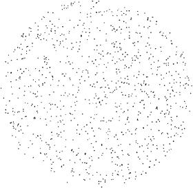
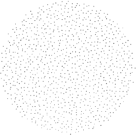
Figure 1.12: Comparison of typical configurations for a completely uncorrelated (Poisson) distribution of 1000 particles (left panel) to the distribution given by the Laughlin wave function for $m=3$ (right panel). The latter is a snapshot taken during a Monte Carlo simulation of the distribution. The Monte Carlo procedure consists of proposing a random trial move of one of the particles to a new position. If this move increases the value of $|\Psi|^{2}$ it is always accepted. If the move decreases the value of $|\Psi|^{2}$ by a factor $p$, then the move is accepted with probability $p$. After equilibration of the plasma by a large number of such moves one finds that the configurations generated are distributed according to $|\Psi|^{2}$. (After R. B. Laughlin, Chap. 7 in [3].)

which shows a typical configuration of particles in the Laughlin ground state (obtained from a Monte Carlo sampling of $|\psi|^{2}$) compared to a random (Poisson) distribution. Focussing first on the large scale features we see that density fluctuations at long wavelengths are severely suppressed in the Laughlin state. This is easily understood in terms of the plasma analogy and the desire for local neutrality. A simple estimate for the density fluctuations $\rho_{\vec{q}}$ at wave vector $\vec{q}$ can be obtained by noting that the fake plasma potential energy can be written (ignoring a constant associated with self-interactions being included)

$$U_{\mathrm{class}}=\frac{1}{2L^{2}}\sum_{\vec{q}\neq 0}\frac{2\pi m^{2}}{q^{2}}\;\rho_{\vec{q}}\rho_{-\vec{q}}$$ (1.116)

where $L^{2}$ is the area of the system and $\frac{2\pi}{q^{2}}$ is the Fourier transform of the logarithmic potential (easily derived from $\nabla^{2}\left(-\ln{(r})\right)=-2\pi\;\delta^{2}(\vec{r}\,)\,$). At long wavelengths $(q^{2}\ll n)$ it is legitimate to treat $\rho_{\vec{q}}$ as a collective coordinate of an elastic continuum. The distribution $e^{-\beta U_{\mathrm{class}}}$ of these coordinates is a gaussian and so obeys (taking into account the fact that $\rho_{-\vec{q}}=(\rho_{\vec{q}})^{*}$)

$$\langle\rho_{\vec{q}}\rho_{-\vec{q}}\rangle=L^{2}\frac{q^{2}}{4\pi m}.$$ (1.117)

We clearly see that the long-range (fake) forces in the (fake) plasma strongly suppress long wavelength density fluctuations. We will return more to this point later when we study collective density wave excitations above the Laughlin ground state.

The density fluctuations on short length scales are best studied in real space. The radial correlation $g(r)$ function is a convenient object to consider. $g(r)$ tells us the density at $r$ given that there is a particle at the origin

$$g(r)=\frac{N(N-1)}{n^{2}Z}\int d^{2}z_{3}\ldots\int d^{2}z_{N}\;\left|\psi(0,r,z_{3},\ldots,z_{N})\right|^{2}$$ (1.118)

where $Z\equiv\langle\psi|\psi\rangle$, $n$ is the density (assumed uniform) and the remaining factors account for all the different pairs of particles that could contribute. The factors of density are included in the denominator so that $\lim_{r\rightarrow\infty}g(r)=1$.

Because the $m=1$ state is a single Slater determinant $g(z)$ can be computed exactly

$$g(z)=1-e^{-\frac{1}{2}|z|^{2}}.$$ (1.119)

Fig. (1.13)

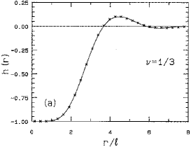
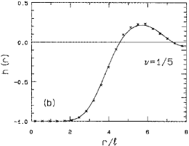
Figure 1.13: Plot of the two-point correlation function $h(r)\equiv 1-g(r)$ for the Laughlin plasma with $\nu^{-1}=m=3$ (left panel) and $m=5$ (right panel). Notice that, unlike the result for $m=1$ given in eq. (1.119), $g(r)$ exhibits the oscillatory behavior characteristic of a strongly coupled plasma with short-range solid-like local order.

shows numerical estimates of $h(r)\equiv 1-g(r)$ for the cases $m=3$ and $5$. Notice that for the $\nu=1/m$ state $g(z)\sim|z|^{2m}$ for small distances. Because of the strong suppression of density fluctuations at long wavelengths, $g(z)$ converges exponentially rapidly to unity at large distances. For $m>1$, $g$ develops oscillations indicative of solid-like correlations and, the plasma actually freezes at $m\approx 65$. The Coulomb interaction energy can be expressed in terms of $g(z)$ as

$$\frac{\langle\psi|V|\psi\rangle}{\langle\psi|\psi\rangle}=\frac{nN}{2}\int d^{2}z\;\frac{e^{2}}{\epsilon|z|}\;\left[g(z)-1\right]$$ (1.120)

where the $(-1)$ term accounts for the neutralizing background and $\epsilon$ is the dielectric constant of the host semiconductor. We can interpret $g(z)-1$ as the density of the ‘exchange-correlation hole’ surrounding each particle.

The correlation energies per particle for $m=3$ and $5$ are [27]

$$\frac{1}{N}\;\frac{\langle\psi_{3}|V|\psi_{3}\rangle}{\langle\psi_{3}|\psi_{3}\rangle}=-0.4100\pm 0.0001$$ (1.121)

and

$$\frac{1}{N}\;\frac{\langle\psi_{5}|V|\psi_{5}\rangle}{\langle\psi_{5}|\psi_{5}\rangle}=-0.3277\pm 0.0002$$ (1.122)

in units of $e^{2}/\epsilon\ell$ which is $\approx 161~{}\mathrm{K}$ for $\epsilon=12.8$ (the value in GaAs), $B=10\mathrm{T}$. For the filled Landau level ($m=1$) the exchange energy is $-\sqrt{\frac{\pi}{8}}$ as can be seen from eqs. (1.119) and (1.120).

Exercise 1.15

Find the radial distribution function for a one-dimensional spinless free electron gas of density $n$ by writing the ground state wave function as a single Slater determinant and then integrating out all but two of the coordinates. Use this first quantization method even if you already know how to do this calculation using second quantization. Hint: Take advantage of the following representation of the determinant of a $N\times N$ matrix $M$ in terms of permutations $P$ of $N$ objects. $$\mathrm{Det}\;M=\sum_{P}(-1)^{P}\prod_{j=1}^{N}M_{jP_{j}}.$$

Exercise 1.16

Using the same method derive eq. (1.119).

1.7 Neutral Collective Excitations

So far we have studied one particular variational wave function and found that it has good correlations built into it as graphically illustrated in Fig. 1.12. To further bolster the case that this wave function captures the physics of the fractional Hall effect we must now demonstrate that there is finite energy cost to produce excitations above this ground state. In this section we will study the neutral collective excitations. We will examine the charged excitations in the next section.

It turns out that the neutral excitations are phonon-like excitations similar to those in solids and in superfluid helium. We can therefore use a simple modification of Feynman’s theory of the excitations in superfluid helium [28, 29].

By way of introduction let us start with the simple harmonic oscillator. The ground state is of the form

$$\psi_{0}(x)\sim e^{-\alpha x^{2}}.$$ (1.123)

Suppose we did not know the excited state and tried to make a variational ansatz for it. Normally we think of the variational method as applying only to ground states. However it is not hard to see that the first excited state energy is given by

$$\epsilon_{1}=\mathrm{min}\,\left\{\frac{\langle\psi|H|\psi\rangle}{\langle\psi|\psi\rangle}\right\}$$ (1.124)

provided that we do the minimization over the set of states $\psi$ which are constrained to be orthogonal to the ground state $\psi_{0}$. One simple way to produce a variational state which is automatically orthogonal to the ground state is to change the parity by multiplying by the first power of the coordinate

$$\psi_{1}(x)\sim x\;e^{-\alpha x^{2}}.$$ (1.125)

Variation with respect to $\alpha$ of course leads (in this special case) to the exact first excited state.

With this background let us now consider the case of phonons in superfluid ${}^{4}\hbox{He}$. Feynman argued that because of the Bose statistics of the particles, there are no low-lying single-particle excitations. This is in stark contrast to a fermi gas which has a high density of low-lying excitations around the fermi surface. Feynman argued that the only low-lying excitations in ${}^{4}\hbox{He}$ are collective density oscillations that are well-described by the following family of variational wave functions (that has no adjustable parameters) labeled by the wave vector

$$\psi_{\vec{k}}=\frac{1}{\sqrt{N}}\;\rho_{\vec{k}}\;\Phi_{0}$$ (1.126)

where $\Phi_{0}$ is the exact ground state and

$$\rho_{\vec{k}}\equiv\sum_{j=1}^{N}e^{-i\vec{k}\cdot\vec{r}_{j}}$$ (1.127)

is the Fourier transform of the density. The physical picture behind this is that at long wavelengths the fluid acts like an elastic continuum and $\rho_{\vec{k}}$ can be treated as a generalized oscillator normal-mode coordinate. In this sense eq. (1.126) is then analogous to eq. (1.125). To see that $\psi_{\vec{k}}$ is orthogonal to the ground state we simply note that

$$\langle\Phi_{0}|\psi_{\vec{k}}\rangle = \frac{1}{\sqrt{N}}\;\langle\Phi_{0}|\rho_{\vec{k}}|\Phi_{0}\rangle$$ (1.128)

$$= \frac{1}{\sqrt{N}}\int d^{3}R\;e^{-i\vec{k}\cdot\vec{R}}\;\langle\Phi_{0}|\rho(\vec{r}\,)|\Phi_{0}\rangle.$$

where

$$\rho(\vec{r}\,)\equiv\sum_{j=1}^{N}\delta^{3}(\vec{r}_{j}-\vec{R})$$ (1.129)

is the density operator. If $\Phi_{0}$ describes a translationally invariant liquid ground state then the Fourier transform of the mean density vanishes for $k\neq 0$.

There are several reasons why $\psi_{\vec{k}}$ is a good variational wave function, especially for small $k$. First, it contains the ground state as a factor. Hence it contains all the special correlations built into the ground state to make sure that the particles avoid close approaches to each other without paying a high price in kinetic energy. Second, $\psi_{\vec{k}}$ builds in the features we expect on physical grounds for a density wave. To see this, consider evaluating $\psi_{\vec{k}}$ for a configuration of the particles like that shown in fig. (1.14a)

Figure 1.14: (a) Configuration of particles in which the Fourier transform of the density at wave vector $k$ is non-zero. (b) The Fourier amplitude will have a similar magnitude for this configuration but a different phase.

which has a density modulation at wave vector $\vec{k}$. This is not a configuration that maximizes $|\Phi_{0}|^{2}$, but as long as the density modulation is not too large and the particles avoid close approaches, $|\Phi_{0}|^{2}$ will not fall too far below its maximum value. More importantly, $|\rho_{\vec{k}}|^{2}$ will be much larger than it would for a more nearly uniform distribution of positions. As a result $|\psi_{\vec{k}}|^{2}$ will be large and this will be a likely configuration of the particles in the excited state. For a configuration like that in fig. (1.14b), the phase of $\rho_{\vec{k}}$ will shift but $|\psi_{\vec{k}}|^{2}$ will have the same magnitude. This is analogous to the parity change in the harmonic oscillator example. Because all different phases of the density wave are equally likely, $\rho_{\vec{k}}$ has a mean density which is uniform (translationally invariant).

To proceed with the calculation of the variational estimate for the excitation energy $\Delta(k)$ of the density wave state we write

$$\Delta(k)=\frac{f(k)}{s(k)}$$ (1.130)

where

$$f(k)\equiv\left\langle\psi_{\vec{k}}|(H-E_{0})|\psi_{\vec{k}}\right\rangle,$$ (1.131)

with $E_{0}$ being the exact ground state energy and

$$s(k)\equiv\langle\psi_{\vec{k}}|\psi_{\vec{k}}\rangle=\frac{1}{N}\;\langle\Phi_{0}|\rho_{\vec{k}}^{\dagger}\rho_{\vec{k}}^{\phantom{\dagger}}|\Phi_{0}\rangle.$$ (1.132)

We see that the norm of the variational state $s(k)$ turns out to be the static structure factor of the ground state. It is a measure of the mean square density fluctuations at wave vector $\vec{k}$. Continuing the harmonic oscillator analogy, we can view this as a measure of the zero-point fluctuations of the normal-mode oscillator coordinate $\rho_{\vec{k}}$. For superfluid ${}^{4}\hbox{He}$ $s(k)$ can be directly measured by neutron scattering and can also be computed theoretically using quantum Monte Carlo methods [30]. We will return to this point shortly.

Exercise 1.17

Show that for a uniform liquid state of density $n$, the static structure factor is related to the Fourier transform of the radial distribution function by $$s(k)=N\;\delta_{\vec{k},\vec{0}}+1+n\int d^{3}r\;e^{i\vec{k}\cdot\vec{r}}\;\left[g(r)-1\right]$$

The numerator in eq. (1.131) is called the oscillator strength and can be written

$$f(k)=\frac{1}{N}\;\left\langle\Phi_{0}|\rho_{\vec{k}}^{\dagger}[H,\rho_{\vec{k}}^{\phantom{\dagger}}]|\Phi_{0}\right\rangle.$$ (1.133)

For uniform systems with parity symmetry we can write this as a double commutator

$$f(k)=\frac{1}{2N}\;\left\langle\Phi_{0}\left|\left[\rho_{\vec{k}}^{\dagger},[H,\rho_{\vec{k}}^{\phantom{\dagger}}]\right]\right|\Phi_{0}\right\rangle$$ (1.134)

from which we can derive the justifiably famous oscillator strength sum rule

$$f(k)=\frac{\hbar^{2}k^{2}}{2M}.$$ (1.135)

where $M$ is the (band) mass of the particles. Remarkably (and conveniently) this is a universal result independent of the form of the interaction potential between the particles. This follows from the fact that only the kinetic energy part of the Hamiltonian fails to commute with the density.

Exercise 1.18

Derive eq. (1.134) and then eq. (1.135) from eq. (1.133) for a system of interacting particles.

We thus arrive at the Feynman-Bijl formula for the collective mode excitation energy

$$\Delta(k)=\frac{\hbar^{2}k^{2}}{2M}\;\frac{1}{s(k)}.$$ (1.136)

We can interpret the first term as the energy cost if a single particle (initially at rest) were to absorb all the momentum and the second term is a renormalization factor describing momentum (and position) correlations among the particles. One of the remarkable features of the Feynman-Bijl formula is that it manages to express a dynamical quantity $\Delta(k)$, which is a property of the excited state spectrum, solely in terms of a static property of the ground state, namely $s(k)$. This is a very powerful and useful approximation.

Returning to eq. (1.126) we see that $\psi_{\vec{k}}$ describes a linear superposition of states in which one single particle has had its momentum boosted by $\hbar\vec{k}$. We do not know which one however. The summation in eq. (1.127) tells us that it is equally likely to be particle 1 or particle 2 or …, etc. This state should not be confused with the state in which boost is applied to particle 1 and particle 2 and …, etc. This state is described by a product

$$\Phi_{\vec{k}}\equiv\left(\prod_{j=1}^{N}e^{i\vec{k}\cdot\vec{r}_{j}}\right)\;\Phi_{0}$$ (1.137)

which can be rewritten

$$\Phi_{\vec{k}}=\exp{\left\{iN\vec{k}\cdot\left(\frac{1}{N}\sum_{j=1}^{N}\vec{r}_{j}\right)\right\}}\;\Phi_{0}$$ (1.138)

showing that this is an exact energy eigenstate (with energy $N\;\frac{\hbar^{2}k^{2}}{2M}$) in which the center of mass momentum has been boosted by $N\hbar\vec{k}$.

In superfluid ${}^{4}\hbox{He}$ the structure factor vanishes linearly at small wave vectors

$$s(k)\sim\xi k$$ (1.139)

so that $\Delta(k)$ is linear as expected for a sound mode

$$\Delta(k)=\left(\frac{\hbar^{2}}{2M}\;\frac{1}{\xi}\right)\;k$$ (1.140)

from which we see that the sound velocity is given by

$$c_{\mathrm{s}}=\frac{\hbar}{2M}\;\frac{1}{\xi}.$$ (1.141)

This phonon mode should not be confused with the ordinary hydrodynamic sound mode in classical fluids. The latter occurs in a collision dominated regime $\omega\tau\ll 1$ in which collision-induced pressure provides the restoring force. The phonon mode described here by $\psi_{\vec{k}}$ is a low-lying eigenstate of the quantum Hamiltonian.

At larger wave vectors there is a peak in the static structure factor caused by the solid-like oscillations in the radial distribution function $g(r)$ similar to those shown in Fig. 1.13 for the Laughlin liquid. This peak in $s(k)$ leads to the so-called roton minimum in $\Delta(k)$ as illustrated in fig. (1.15).

Figure 1.15: Schematic illustration of the phonon dispersion in superfluid liquid ⁴He. For small wave vectors the dispersion is linear, as is expected for a gapless Goldstone mode. The roton minimum due to the peak in the static structure factor occurs at a wave vector $k$ of approximately 20 in units of inverse Å. The roton energy is approximately $10$ in units of Kelvins.

To better understand the Feynman picture of the collective excited states recall that the dynamical structure factor is defined (at zero temperature) by

$$S(q,\omega)\equiv\frac{2\pi}{N}\;\left\langle\Phi_{0}\left|\rho_{\vec{q}}^{\dagger}\;\,\delta\left(\omega-\frac{H-E_{0}}{\hbar}\right)\rho_{\vec{q}}^{\phantom{\dagger}}\right|\Phi_{0}\right\rangle.$$ (1.142)

The static structure factor is the zeroth frequency moment

$$s(q)=\int_{-\infty}^{\infty}\frac{d\omega}{2\pi}\;S(q,\omega)=\int_{0}^{\infty}\frac{d\omega}{2\pi}\;S(q,\omega)$$ (1.143)

(with the second equality valid only at zero temperature). Similarly the oscillator strength in eq. (1.131) becomes (at zero temperature)

$$f(q)=\int_{-\infty}^{\infty}\frac{d\omega}{2\pi}\;\hbar\omega\;S(q,\omega)=\int_{0}^{\infty}\frac{d\omega}{2\pi}\;\hbar\omega\;S(q,\omega).$$ (1.144)

Thus we arrive at the result that the Feynman-Bijl formula can be rewritten

$$\Delta(q)=\frac{\int_{0}^{\infty}\frac{d\omega}{2\pi}\;\hbar\omega\;S(q,\omega)}{\int_{0}^{\infty}\frac{d\omega}{2\pi}\;S(q,\omega)}.$$ (1.145)

That is, $\Delta(q)$ is the mean excitation energy (weighted by the square of the density operator matrix element). Clearly the mean exceeds the minimum and so the estimate is variational as claimed. Feynman’s approximation is equivalent to the assumption that only a single mode contributes any oscillator strength so that the zero-temperature dynamical structure factor contains only a single delta function peak

$$S(q,\omega)=2\pi\;s(q)\;\delta\left(\omega-\frac{1}{\hbar}\;\Delta(q)\right).$$ (1.146)

Notice that this approximate form satisfies both eq. (1.143) and eq. (1.144) provided that the collective mode energy $\Delta(q)$ obeys the Feynman-Bijl formula in eq. (1.136).

Exercise 1.19

For a system with a homogeneous liquid ground state, the (linear response) static susceptibility of the density to a perturbation $U=V_{\vec{q}}\rho_{-\vec{q}}$ is defined by $$\left\langle\rho_{\vec{q}}\right\rangle=\chi(q)V_{\vec{q}}.$$ (1.147) Using first order perturbation theory show that the static susceptibility is given in terms of the dynamical structure factor by $$\chi(q)=-2\int_{0}^{\infty}\frac{d\omega}{2\pi}\frac{1}{\hbar\omega}S(q,\omega).$$ (1.148) Using the single mode approximation and the oscillator strength sum rule, derive an expression for the collective mode dispersion in terms of $\chi(q)$. (Your answer should not involve the static structure factor. Note also that eq.(1.147) is not needed to produce the answer to this part. Just work with eq.(1.148).)

As we mentioned previously Feynman argued that in ${}^{4}\hbox{He}$ the Bose symmetry of the wave functions guarantees that unlike in Fermi systems, there is only a single low-lying mode, namely the phonon density mode. The paucity of low-energy single particle excitations in boson systems is what helps make them superfluid–there are no dissipative channels for the current to decay into. Despite the fact that the quantum Hall system is made up of fermions, the behavior is also reminiscent of superfluidity since the current flow is dissipationless. Indeed, within the ‘composite boson’ picture, one views the FQHE ground state as a bose condensate [1, 9, 10]. Let us therefore blindly make the single-mode approximation and see what happens.

From eq. (1.117) we see that the static structure factor for the $m$th Laughlin state is (for small wave vectors only)

$$s(q)=\frac{L^{2}}{N}\;\frac{q^{2}}{4\pi m}=\frac{1}{2}\;q^{2}\ell^{2},$$ (1.149)

where we have used $L^{2}/N=2\pi\ell^{2}m$. The Feynman-Bijl formula then yields

$$\Delta(q)=\frac{\hbar^{2}q^{2}}{2M}\;\frac{2}{q^{2}\ell^{2}}=\hbar\omega_{c}.$$ (1.150)

This predicts that there is an excitation gap that is independent of wave vector (for small $q$) and equal to the cyclotron energy. It is in fact correct that at long wavelengths the oscillator strength is dominated by transitions in which a single particle is excited from the $n=0$ to the $n=1$ Landau level. Furthermore, Kohn’s theorem guarantees that the mode energy is precisely $\hbar\omega_{c}$. Eq. (1.150) was derived specifically for the Laughlin state, but it is actually quite general, applying to any translationally invariant liquid ground state.

One might expect that the single mode approximation (SMA) will not work well in an ordinary Fermi gas due to the high density of excitations around the Fermi surface. Here however the Fermi surface has been destroyed by the magnetic field and the continuum of excitations with different kinetic energies has been turned into a set of discrete inter-Landau-level excitations, the lowest of which dominates the oscillator strength.

For filling factor $\nu=1$ the Pauli principle prevents any intra-level excitations and the excitation gap is in fact $\hbar\omega_{c}$ as predicted by the SMA. However for $\nu<1$ there should exist intra-Landau-level excitations whose energy scale is set by the interaction scale $e^{2}/\epsilon\ell$ rather than the kinetic energy scale $\hbar\omega_{c}$. Indeed we can formally think of taking the band mass to zero ($M\rightarrow 0$) which would send $\hbar\omega_{c}\rightarrow\infty$ while keeping $e^{2}/\epsilon\ell$ fixed. Unfortunately the SMA as it stands now is not very useful in this limit. What we need is a variational wave function that represents a density wave but is restricted to lie in the Hilbert space of the lowest Landau level. This can be formally accomplished by replacing eq. (1.126) by

$$\psi_{\vec{k}}=\bar{\rho}_{\vec{k}}\;\psi_{m}$$ (1.151)

where the overbar indicates that the density operator has been projected into the lowest Landau level. The details of how this is accomplished are presented in appendix A.

The analog of eq. (1.130) is

$$\Delta(k)=\frac{\bar{f}(k)}{\bar{s}(k)}$$ (1.152)

where $\bar{f}$ and $\bar{s}$ are the projected oscillator strength and structure factor, respectively. As shown in appendix A

$$\bar{s}(k) \equiv \frac{1}{N}\;\left\langle\psi_{m}|\bar{\rho}_{\vec{k}}^{\dagger}\;\bar{\rho}_{\vec{k}}|\psi_{m}\right\rangle=s(k)-\left[1-e^{-\frac{1}{2}|k|^{2}\ell^{2}}\right]$$ (1.153)

$$= s(k)-s_{\nu=1}(k).$$

This vanishes for the filled Landau level because the Pauli principle forbids all intra-Landau-level excitations. For the $m$th Laughlin state eq. (1.149) shows us that the leading term in $s(k)$ for small $k$ is $\frac{1}{2}k^{2}\ell^{2}$. Putting this into eq. (1.153) we see that the leading behavior for $\bar{s}(k)$ is therefore quartic

$$\bar{s}(k)\sim a(k\ell)^{4}+\ldots.$$ (1.154)

We can not compute the coefficient $a$ without finding the $k^{4}$ correction to eq. (1.149). It turns out that there exists a compressibility sum rule for the fake plasma from which we can obtain the exact result [29]

$$a=\frac{m-1}{8}.$$ (1.155)

The projected oscillator strength is given by eq. (1.134) with the density operators replaced by their projections. In the case of ${}^{4}\hbox{He}$ only the kinetic energy part of the Hamiltonian failed to commute with the density. It was for this reason that the oscillator strength came out to be a universal number related to the mass of the particles. Within the lowest Landau level however the kinetic energy is an irrelevant constant. Instead, after projection the density operators no longer commute with each other (see appendix A). It follows from these commutation relations that the projected oscillator strength is proportional to the strength of the interaction term. The leading small $k$ behavior is [29]

$$\bar{f}(k)=b\;\frac{e^{2}}{\epsilon\ell}(k\ell)^{4}+\ldots$$ (1.156)

where $b$ is a dimensionless constant that depends on the details of the interaction potential. The intra-Landau level excitation energy therefore has a finite gap at small $k$

$$\Delta(k)=\frac{\bar{f}(k)}{\bar{s}(k)}\sim\frac{b}{a}\;\frac{e^{2}}{\epsilon\ell}+\mathcal{O}(k^{2})+\ldots$$ (1.157)

This is quite different from the case of superfluid ${}^{4}\hbox{He}$ in which the mode is gapless. However like the case of the superfluid, this ‘magnetophonon’ mode has a ‘magnetoroton’ minimum at finite $k$ as illustrated in fig. (1.16).

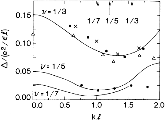
Figure 1.16: Comparison of the single mode approximation (SMA) prediction of the collective mode energy for filling factors $\nu=1/3,1/5,1/7$ (solid lines) with small-system numerical results for $N$ particles. Crosses indicate the $N=7,\nu=1/3$ spherical system, triangles indicate the $N=6,\nu=1/3$ hexagonal unit cell system results of Haldane and Rezayi [31]. Solid dots are for $N=9,\nu=1/3$ and $N=7,\nu=1/5$ spherical system calculations of Fano et al. [32] Arrows at the top indicate the magnitude of the reciprocal lattice vector of the Wigner crystal at the corresponding filling factor. Notice that unlike the phonon collective mode in superfluid helium shown in fig. (1.15), the mode here is gapped.

The figure also shows results from numerical exact diagonalization studies which demonstrate that the single mode approximation is extremely accurate. Note that the magnetoroton minimum occurs close to the position of the smallest reciprocal lattice vector in the Wigner crystal of the same density. In the crystal the phonon frequency would go exactly to zero at this point. (Recall that in a crystal the phonon dispersion curves have the periodicity of the reciprocal lattice.)

Because the oscillator strength is almost entirely in the cyclotron mode, the dipole matrix element for coupling the collective excitations to light is very small. They have however been observed in Raman scattering [33] and found to have an energy gap in excellent quantitative agreement with the single mode approximation.

Finally we remark that these collective excitations are characterized by a well-defined wave vector $\vec{k}$ despite the presence of the strong magnetic field. This is only possible because they are charge neutral which allows one to define a gauge invariant conserved momentum [34].

1.8 Charged Excitations

Except for the fact that they are gapped, the neutral magnetophonon excitations are closely analogous to the phonon excitations in superfluid ${}^{4}\hbox{He}$. We further pursue this analogy with a search for the analog of vortices in superfluid films. A vortex is a topological defect which is the quantum version of the familiar whirlpool. A reasonably good variational wave function for a vortex in a two-dimensional film of ${}^{4}\hbox{He}$ is

$$\psi_{\vec{R}}^{\pm}=\left\{\prod_{j=1}^{N}f\left(|\vec{r}_{j}-\vec{R}|\right)\;e^{\pm i\theta(\vec{r}_{j}-\vec{R})}\right\}\Phi_{0}.$$ (1.158)

Here $\theta$ is the azimuthal angle that the particle’s position makes relative to $\vec{R}$, the location of the vortex center. The function $f$ vanishes as $\vec{r}$ approaches $\vec{R}$ and goes to unity far away. The choice of sign in the phase determines whether the vortex is right or left handed.

The interpretation of this wave function is the following. The vortex is a topological defect because if any particle is dragged around a closed loop surrounding $\vec{R}$, the phase of the wave function winds by $\pm 2\pi$. This phase gradient means that current is circulating around the core. Consider a large circle of radius $\xi$ centered on $\vec{R}$. The phase change of $2\pi$ around the circle occurs in a distance $2\pi\xi$ so the local gradient seen by every particle is $\hat{\theta}/\xi$. Recalling eq. (1.138) we see that locally the center of mass momentum has been boosted by $\pm\frac{\hbar}{\xi}\;\hat{\theta}$ so that the current density of the whirlpool falls off inversely with distance from the core. Near the core $f$ falls to zero because of the ‘centrifugal barrier’ associated with this circulation. In a more accurate variational wave function the core would be treated slightly differently but the asymptotic large distance behavior would be unchanged.

What is the analog of all this for the lowest Landau level? For $\psi^{+}$ we see that every particle has its angular momentum boosted by one unit. In the lowest Landau level analyticity (in the symmetric gauge) requires us to replace $e^{i\theta}$ by $z=x+iy$. Thus we are led to the Laughlin ‘quasi-hole’ wave function

$$\psi_{Z}^{+}[z]=\prod_{j=1}^{N}(z_{j}-Z)\;\psi_{m}[z]$$ (1.159)

where $Z$ is a complex number denoting the position of the vortex and $\psi_{m}$ is the Laughlin wave function at filling factor $\nu=1/m$. The corresponding antivortex (‘quasi-electron’ state) involves $z_{j}^{*}$ suitably projected (as discussed in App. A.):

$$\psi_{Z}^{-}[z]=\prod_{j=1}^{N}\left(2\frac{\partial}{\partial z_{j}}-Z^{*}\right)\;\psi_{m}[z]$$ (1.160)

where as usual the derivatives act only on the polynomial part of $\psi_{m}$. All these derivatives make $\psi^{-}$ somewhat difficult to work with. We will therefore concentrate on the quasi-hole state $\psi^{+}$. The origin of the names quasi-hole and quasi-electron will become clear shortly.

Unlike the case of a superfluid film, the presence of the vector potential allows these vortices to cost only a finite energy to produce and hence the electrical dissipation is always finite at any non-zero temperature. There is no finite temperature transition into a superfluid state as in the Kosterlitz Thouless transition. From a field theoretic point of view, this is closely analogous to the Higg’s mechanism [1].

Just as in our study of the Laughlin wave function, it is very useful to see how the plasma analogy works for the quasi-hole state

$$|\psi_{Z}^{+}|^{2}=e^{-\beta U_{\mathrm{class}}}\;e^{-\beta V}$$ (1.161)

where $U_{\mathrm{class}}$ is given by eq. (1.98), $\beta=2/m$ as before and

$$V\equiv m\sum_{j=1}^{N}\left(-\ln{|z_{j}-Z|}\right).$$ (1.162)

Thus we have the classical statistical mechanics of a one-component plasma of (fake) charge $m$ objects seeing a neutralizing jellium background plus a new potential energy $V$ representing the interaction of these objects with an ‘impurity’ located at $Z$ and having unit charge.

Recall that the chief desire of the plasma is to maintain charge neutrality. Hence the plasma particles will be repelled from $Z$. Because the plasma particles have fake charge $m$, the screening cloud will have to have a net reduction of $1/m$ particles to screen the impurity. But this means that the quasi-hole has fractional fermion number! The (true) physical charge of the object is a fraction of the elementary charge

$$q^{*}=\frac{e}{m}.$$ (1.163)

This is very strange! How can we possibly have an elementary excitation carrying fractional charge in a system made up entirely of electrons? To understand this let us consider an example of another quantum system that seems to have fractional charge, but in reality doesn’t. Imagine three protons arranged in an equilateral triangle as shown in fig. (1.17).

Figure 1.17: Illustration of an electron tunneling among the 1S orbitals of three protons. The tunneling is exponentially slow for large separations which leads to only exponentially small lifting of what would otherwise be a three-fold degenerate ground state.

Let there be one electron in the system. In the spirit of the tight-binding model we consider only the 1S orbital on each of the three ‘lattice sites’. The Bloch states are

$$\psi_{k}=\frac{1}{\sqrt{3}}\sum_{j=1}^{3}e^{ikj}\;|j\rangle$$ (1.164)

where $|j\rangle$ is the 1S orbital for the $j$th atom. The equilateral triangle is like a linear system of length 3 with periodic boundary conditions. Hence the allowed values of the wavevector are $\left\{k_{\alpha}=\frac{2\pi}{3}\alpha;\;\;\alpha=-1,0,+1\right\}$. The energy eigenvalues are

$$\epsilon_{k_{\alpha}}=-E_{\mathrm{1S}}-2J\;\cos{k_{\alpha}}$$ (1.165)

where $E_{\mathrm{1S}}$ is the isolated atom energy and $-J$ is the hopping matrix element related to the orbital overlap and is exponentially small for large separations of the atoms.

The projection operator that measures whether or not the particle is on site $n$ is

$$P_{n}\equiv|n\rangle\;\langle n|.$$ (1.166)

Its expectation value in any of the three eigenstates is

$$\left\langle\psi_{k_{\alpha}}|P_{n}|\psi_{k_{\alpha}}\right\rangle=\frac{1}{3}.$$ (1.167)

This equation simply reflects the fact that as the particle tunnels from site to site it is equally likely to be found on any site. Hence it will, on average, be found on a particular site $n$ only 1/3 of the time. The average electron number per site is thus 1/3. This however is a trivial example because the value of the measured charge is always an integer. Two-thirds of the time we measure zero and one third of the time we measure unity. This means that the charge fluctuates. One measure of the fluctuations is

$$\sqrt{\langle P_{n}^{2}\rangle-\langle P_{n}\rangle^{2}}=\sqrt{\frac{1}{3}-\frac{1}{9}}=\frac{\sqrt{2}}{3},$$ (1.168)

which shows that the fluctuations are larger than the mean value. This result is most easily obtained by noting $P_{n}^{2}=P_{n}$.

A characteristic feature of this ‘imposter’ fractional charge $\frac{e}{m}$ that guarantees that it fluctuates is the existence in the spectrum of the Hamiltonian of a set of $m$ nearly degenerate states. (In our toy example here, $m=3$.) The characteristic time scale for the charge fluctuations is $\tau\sim\hbar/\Delta\epsilon$ where $\Delta\epsilon$ is the energy splitting of the quasi-degenerate manifold of states. In our tight-binding example $\tau\sim\hbar/J$ is the characteristic time it takes an electron to tunnel from the 1S orbital on one site to the next. As the separation between the sites increases this tunneling time grows exponentially large and the charge fluctuations become exponentially slow and thus easy to detect.

In a certain precise sense, the fractional charge of the Laughlin quasiparticles behaves very differently from this. An electron added at low energies to a $\nu=1/3$ quantum Hall fluid breaks up into three charge 1/3 Laughlin quasiparticles. These quasiparticles can move arbitrarily far apart from each other and yet no quasi-degenerate manifold of states appears. The excitation gap to the first excited state remains finite. The only degeneracy is that associated with the positions of the quasiparticles. If we imagine that there are three impurity potentials that pin down the positions of the three quasiparticles, then the state of the system is uniquely specified. Because there is no quasidegeneracy, we do not have to specify any more information other than the positions of the quasiparticles. Hence in a deep sense, they are true elementary particles whose fractional charge is a sharp quantum observable.

Of course, since the system is made up only of electrons, if we capture the charges in some region in a box, we will always get an integer number of electrons inside the box. However in order to close the box we have to locally destroy the Laughlin state. This will cost (at a minimum) the excitation gap. This may not seem important since the gap is small — only a few Kelvin or so. But imagine that the gap were an MeV or a GeV. Then we would have to build a particle accelerator to ‘close the box’ and probe the fluctuations in the charge. These fluctuations would be analogous to the ones seen in quantum electrodynamics at energies above $2m_{e}c^{2}$ where electron-positron pairs are produced during the measurement of charge form factors by means of a scattering experiment.

Put another way, the charge of the Laughlin quasiparticle fluctuates but only at high frequencies $\sim\Delta/\hbar$. If this frequency (which is $\sim 50\hbox{GHz}$) is higher than the frequency response limit of our voltage probes, we will see no charge fluctuations. We can formalize this by writing a modified projection operator [35] for the charge on some site $n$ by

$$P_{n}^{(\Omega)}\equiv P^{\Omega}\;P_{n}P^{\Omega}$$ (1.169)

where $P_{n}=|n\rangle\;\langle n|$ as before and

$$P^{(\Omega)}\equiv\theta(\Omega-H+E_{0})$$ (1.170)

is the operator that projects onto the subset of eigenstates with excitation energies less than $\Omega$. $P_{n}^{(\Omega)}$ thus represents a measurement with a high-frequency cutoff built in to represent the finite bandwidth of the detector. Returning to our tight-binding example, consider the situation where $J$ is large enough that the excitation gap $\Delta=\left(1-\cos{\frac{2\pi}{3}}\right)J$ exceeds the cutoff $\Omega$. Then

$$P^{(\Omega)} = \sum_{\alpha=-1}^{+1}|\psi_{k_{\alpha}}\rangle\;\theta(\Omega-\epsilon_{k_{\alpha}}+\epsilon_{k_{0}})\;\langle\psi_{k_{\alpha}}|$$ (1.171)

$$= |\psi_{k_{0}}\rangle\;\langle\psi_{k_{0}}|$$

is simply a projector on the ground state. In this case

$$P_{n}^{(\Omega)}=|\psi_{k_{0}}\rangle\;\frac{1}{3}\;\langle\psi_{k_{0}}|$$ (1.172)

and

$$\left\langle\psi_{k_{0}}\left|[P_{n}^{(\Omega)}]^{2}\right|\psi_{k_{0}}\right\rangle-\left\langle\psi_{k_{0}}|P_{n}^{(\Omega)}|\psi_{k_{0}}\right\rangle^{2}=0.$$ (1.173)

The charge fluctuations in the ground state are then zero (as measured by the finite bandwidth detector).

The argument for the Laughlin quasiparticles is similar. We again emphasize that one can not think of a single charge tunneling among three sites because the excitation gap remains finite no matter how far apart the quasiparticle sites are located. This is possible only because it is a correlated many-particle system.

To gain a better understanding of fractional charge it is useful to compare this situation to that in high energy physics. In that field of study one knows the physics at low energies — this is just the phenomena of our everyday world. The goal is to study the high energy (short length scale) limit to see where this low energy physics comes from. What force laws lead to our world? Probing the proton with high energy electrons we can temporarily break it up into three fractionally charged quarks, for example.

Condensed matter physics in a sense does the reverse. We know the phenomena at ‘high’ energies (i.e. room temperature) and we would like to see how the known dynamics (Coulomb’s law and non-relativistic quantum mechanics) leads to unknown and surprising collective effects at low temperatures and long length scales. The analog of the particle accelerator is the dilution refrigerator.

To further understand Laughlin quasiparticles consider the point of view of ‘flatland’ physicists living in the cold, two-dimensional world of a $\nu=1/3$ quantum Hall sample. As far as the flatlanders are concerned the ‘vacuum’ (the Laughlin liquid) is completely inert and featureless. They discover however that the universe is not completely empty. There are a few elementary particles around, all having the same charge $q$. The flatland equivalent of Benjamin Franklin chooses a unit of charge which not only makes $q$ negative but gives it the fractional value $-1/3$. For some reason the Flatlanders go along with this.

Flatland cosmologists theorize that these objects are ‘cosmic strings’, topological defects left over from the ‘big cool down’ that followed the creation of the universe. Flatland experimentalists call for the creation of a national accelerator facility which will reach the unprecedented energy scale of 10 Kelvin. With great effort and expense this energy scale is reached and the accelerator is used to smash together three charged particles. To the astonishment of the entire world a new short-lived particle is temporarily created with the bizarre property of having integer charge!

There is another way to see that the Laughlin quasiparticles carry fractional charge which is useful to understand because it shows the deep connection between the sharp fractional charge and the sharp quantization of the Hall conductivity. Imagine piercing the sample with an infinitely thin magnetic solenoid as shown in fig. (1.18)

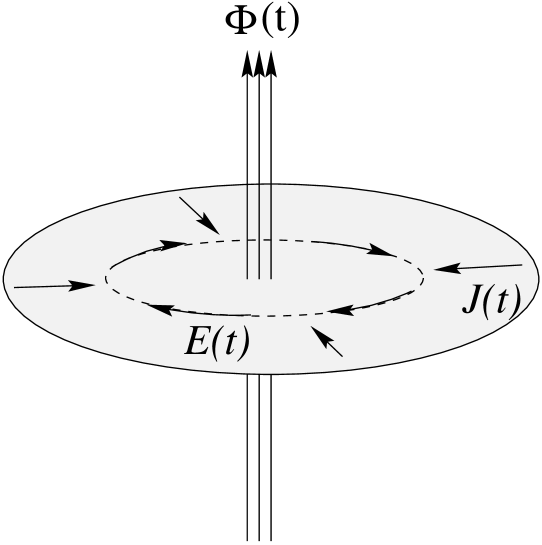
Figure 1.18: Construction of a Laughlin quasiparticle by adiabatically threading flux $\Phi(t)$ through a point in the sample. Faraday induction gives an azimuthal electric field $E(t)$ which in turn produces a radial current $J(t)$. For each quantum of flux added, charge $\nu e$ flows into (or out of) the region due to the quantized Hall conductivity $\nu e^{2}/h$. A flux tube containing an integer number of flux quanta is invisible to the particles (since the Aharanov phase shift is an integer multiple of $2\pi$) and so can be removed by a singular gauge transformation.

and slowly increasing the magnetic flux $\Phi$ from 0 to $\Phi_{0}=\frac{hc}{e}$ the quantum of flux. Because of the existence of a finite excitation gap $\Delta$ the process is adiabatic and reversible if performed slowly on a time scale long compared to $\hbar/\Delta$.

Faraday’s law tells us that the changing flux induces an electric field obeying

$$\oint_{\Gamma}d\vec{r}\cdot\vec{E}=-\frac{1}{c}\;\frac{\partial\Phi}{\partial t}$$ (1.174)

where $\Gamma$ is any contour surrounding the flux tube. Because the electric field contains only Fourier components at frequencies $\omega$ obeying $\hbar\omega<\Delta$, there is no dissipation and $\sigma_{xx}=\sigma_{yy}=\rho_{xx}=\rho_{yy}=0$. The electric field induces a current density obeying

$$\vec{E}=\rho_{xy}\;\vec{J}\times\hat{z}$$ (1.175)

so that

$$\rho_{xy}\oint_{\Gamma}\vec{J}\cdot(\hat{z}\times d\vec{r})=-\frac{1}{c}\;\frac{d\Phi}{dt}.$$ (1.176)

The integral on the LHS represents the total current flowing into the region enclosed by the contour. Thus the charge inside this region obeys

$$\rho_{xy}\;\frac{dQ}{dt}=-\frac{1}{c}\;\frac{d\Phi}{dt}.$$ (1.177)

After one quantum of flux has been added the final charge is

$$Q=\frac{1}{c}\;\sigma_{xy}\Phi_{0}=\frac{h}{e}\;\sigma_{xy}.$$ (1.178)

Thus on the quantized Hall plateau at filling factor $\nu$ where $\sigma_{xy}=\nu\;\frac{e^{2}}{h}$ we have the result

$$Q=\nu e.$$ (1.179)

Reversing the sign of the added flux would reverse the sign of the charge.

The final step in the argument is to note that an infinitesimal tube containing a quantum of flux is invisible to the particles. This is because the Aharonov-Bohm phase factor for traveling around the flux tube is unity.

$$\exp{\left\{i\frac{e}{\hbar c}\oint_{\Gamma}\delta\vec{A}\cdot d\vec{r}\right\}}=e^{\pm 2\pi i}=1.$$ (1.180)

Here $\delta\vec{A}$ is the additional vector potential due to the solenoid. Assuming the flux tube is located at the origin and making the gauge choice

$$\delta\vec{A}=\Phi_{0}\;\frac{\hat{\theta}}{2\pi r},$$ (1.181)

one can see by direct substitution into the Schrödinger equation that the only effect of the quantized flux tube is to change the phase of the wave function by

$$\psi\rightarrow\psi\prod_{j}\frac{z_{j}}{|z_{j}|}=\psi\prod_{j}e^{i\theta_{j}}.$$ (1.182)

The removal of a quantized flux tube is thus a ‘singular gauge change’ which has no physical effect.

Let us reiterate. Adiabatic insertion of a flux quantum changes the state of the system by pulling in (or pushing out) a (fractionally) quantized amount of charge. Once the flux tube contains a quantum of flux it effectively becomes invisible to the electrons and can be removed by means of a singular gauge transformation.

Because the excitation gap is preserved during the adiabatic addition of the flux, the state of the system is fully specified by the position of the resulting quasiparticle. As discussed before there are no low-lying quasi-degenerate states. This version of the argument highlights the essential importance of the fact that $\sigma_{xx}=0$ and $\sigma_{xy}$ is quantized. The existence of the fractionally quantized Hall transport coefficients guarantees the existence of fractionally charged elementary excitations

These fractionally charged objects have been observed directly by using an ultrasensitive electrometer made from a quantum dot [36] and by the reduced shot noise which they produce when they carry current [37].

Because the Laughlin quasiparticles are discrete objects they cost a non-zero (but finite) energy to produce. Since they are charged they can be thermally excited only in neutral pairs. The charge excitation gap is therefore

$$\Delta_{c}=\Delta_{+}+\Delta_{-}$$ (1.183)

where $\Delta_{\pm}$ is the vortex/antivortex (quasielectron/quasihole) excitation energy. In the presence of a transport current these thermally excited charges can move under the influence of the Hall electric field and dissipate energy. The resulting resistivity has the Arrhenius form

$$\rho_{xx}\sim\gamma\frac{h}{e^{2}}\;e^{-\beta\Delta_{c}/2}$$ (1.184)

where $\gamma$ is a dimensionless constant of order unity. Note that the law of mass action tells us that the activation energy is $\Delta_{c}/2$ not $\Delta_{c}$ since the charges are excited in pairs. There is a close analogy between the dissipation described here and the flux flow resistance caused by vortices in a superconducting film.

Theoretical estimates of $\Delta_{c}$ are in good agreement with experimental values determined from transport measurements [38]. Typical values of $\Delta_{c}$ are only a few percent of $e^{2}/\epsilon\ell$ and hence no larger than a few Kelvin. In a superfluid time-reversal symmetry guarantees that vortices and antivortices have equal energies. The lack of time reversal symmetry here means that $\Delta_{+}$ and $\Delta_{-}$ can be quite different. Consider for example the hard-core model for which the Laughlin wave function $\psi_{m}$ is an exact zero energy ground state as shown in eq. (1.114). Equation (1.159) shows that the quasihole state contains $\psi_{m}$ as a factor and hence is also an exact zero energy eigenstate for the hard-core interaction. Thus the quasihole costs zero energy. On the other hand eq. (1.160) tells us that the derivatives reduce the degree of homogeneity of the Laughlin polynomial and therefore the energy of the quasielectron must be non-zero in the hard-core model. At filling factor $\nu=1/m$ this asymmetry has no particular significance since the quasiparticles must be excited in pairs.

Consider now what happens when the magnetic field is increased slightly or the particle number is decreased slightly so that the filling factor is slightly smaller than $1/m$. The lowest energy way to accommodate this is to inject $m$ quasiholes into the Laughlin state for each electron that is removed (or for each $m\Phi_{0}$ of flux that is added). The system energy (ignoring disorder and interactions in the dilute gas of quasiparticles) is

$$E_{+}=E_{m}-\delta N\;m\Delta_{+}$$ (1.185)

where $E_{m}$ is the Laughlin ground state energy and $-\delta N$ is the number of added holes. Conversely for filling factors slightly greater than $1/m$ the energy is (with $+\delta N$ being the number of added electrons)

$$E_{-}=E_{m}+\delta N\;m\Delta_{-}.$$ (1.186)

This is illustrated in fig. (1.19).

Figure 1.19: Energy cost for inserting $\delta N$ electrons into the Laughlin state near filling factor $\nu=1/m$. The slope of the line is the chemical potential. Its discontinuity at $\nu=1/m$ measures the charge excitation gap.

The slope of the lines in the figure determines the chemical potential

$$\mu_{\pm}=\frac{\partial E_{\pm}}{\partial\delta N}=\mp m\Delta_{\pm}.$$ (1.187)

The chemical potential suffers a jump discontinuity of $m(\Delta_{+}+\Delta_{-})=m\Delta_{c}$ just at filling factor $\mu=1/m$. This jump in the chemical potential is the signature of the charge excitation gap just as it is in a semiconductor or insulator. Notice that this form of the energy is very reminiscent of the energy of a type-II superconductor as a function of the applied magnetic field (which induces vortices and therefore has an energy cost $\Delta E\sim|B|$).

Recall that in order to have a quantized Hall plateau of finite width it is necessary to have disorder present. For the integer case we found that disorder localizes the excess electrons allowing the transport coefficients to not change with the filling factor. Here it is the fractionally-charged quasiparticles that are localized by the disorder. Just as in the integer case the disorder may fill in the gap in the density of states but the DC value of $\sigma_{xx}$ can remain zero because of the localization. Thus the fractional plateaus can have finite width.

If the density of quasiparticles becomes too high they may delocalize and condense into a correlated Laughlin state of their own. This gives rise to a hierarchical family of Hall plateaus at rational fractional filling factors $\nu=p/q$ (generically with $q$ odd due to the Pauli principle). There are several different but entirely equivalent ways of constructing and viewing this hierarchy which we will not delve into here [3, 4, 6].

1.9 FQHE Edge States

We learned in our study of the integer QHE that gapless edge excitations exist even when the bulk has a large excitation gap. Because the bulk is incompressible the only gapless neutral excitations must be area-preserving shape distortions such as those illustrated for a disk geometry in fig. (1.20a).

Figure 1.20: Area-preserving shape distortions of the incompressible quantum Hall state. (a) IQHE Laughlin liquid ‘droplet’ at $\nu=1$. (b) FQHE annulus at $\nu=1/m$ formed by injecting a large number $n$ of flux quanta at the origin to create $n$ quasiholes. There are thus two edge modes of opposite chirality. Changing $n$ by one unit transfers fractional charge $\nu e$ from one edge to the other by expanding or shrinking the size of the central hole. Thus the edge modes have topological sectors labeled by the ‘winding number’ $n$ and one can view the gapless edge excitations as a gas of fractionally charged Laughlin quasiparticles.

Because of the confining potential at the edges these shape distortions have a characteristic velocity produced by the $\vec{E}\times\vec{B}$ drift. It is possible to show that this view of the gapless neutral excitations is precisely equivalent to the usual Fermi gas particle-hole pair excitations that we considered previously in our discussion of edge states. Recall that we argued that the contour line of the electrostatic potential separating the occupied from the empty states could be viewed as a real-space analog of the Fermi surface (since position and momentum are equivalent in the Landau gauge). The charged excitations at the edge are simply ordinary electrons added or removed from the vicinity of the edge.

In the case of a fractional QHE state at $\nu=1/m$ the bulk gap is caused by Coulomb correlations and is smaller but still finite. Again the only gapless excitations are area-preserving shape distortions. Now however the charge of each edge can be varied in units of $e/m$. Consider the annulus of Hall fluid shown in fig. (1.20b). The extension of the Laughlin wave function $\psi_{m}$ to this situation is

$$\psi_{mn}[z]=\left(\prod_{j=1}^{N}z_{j}^{n}\right)\;\psi_{m}.$$ (1.188)

This simply places a large number $n\gg 1$ of quasiholes at the origin. Following the plasma analogy we see that this looks like a highly charged impurity at the origin which repels the plasma, producing the annulus shown in fig. (1.20b). Each time we increase $n$ by one unit, the annulus expands. We can view this expansion as increasing the electron number at the outer edge by $1/m$ and reducing it by $1/m$ at the inner edge. (Thereby keeping the total electron number integral as it must be.)

It is appropriate to view the Laughlin quasiparticles, which are gapped in the bulk, as being liberated at the edge. The gapless shape distortions in the Hall liquid are thus excitations in a ‘gas’ of fractionally charged quasiparticles. This fact produces a profound alteration in the tunneling density of states to inject an electron into the system. An electron which is suddenly added to an edge (by tunneling through a barrier from an external electrode) will have very high energy unless it breaks up into $m$ Laughlin quasiparticles. This leads to an ‘orthogonality catastrophe’ which simply means that the probability for this process is smaller and smaller for final states of lower and lower energy. As a result the current-voltage characteristic for the tunnel junction becomes non-linear [17, 39, 40]

$$I\sim V^{m}.$$ (1.189)

For the filled Landau level $m=1$ the quasiparticles have charge $q=em=e$ and are ordinary electrons. Hence there is no orthogonality catastrophe and the I-V characteristic is linear as expected for an ordinary metallic tunnel junction. The non-linear tunneling for the $m=3$ state is shown in fig. (1.21).

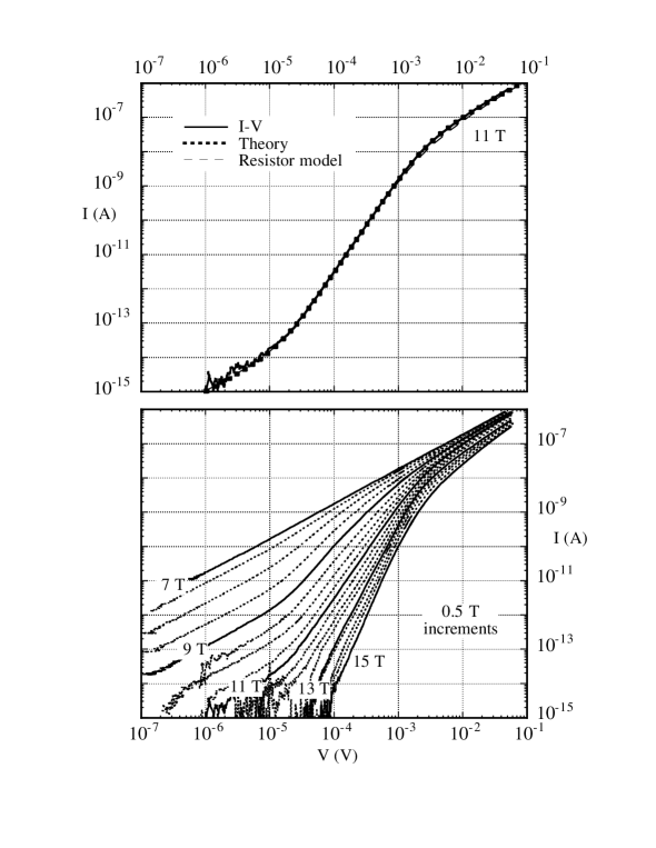
Figure 1.21: Non-linear current voltage response for tunneling an electron into a FQHE edge state. Because the electron must break up into $m$ fractionally charged quasiparticles, there is an orthogonality catastrophe leading to a power-law density of states. The flattening at low currents is due to the finite temperature. The upper panel shows the $\nu=1/3$ Hall plateau. The theory [17, 39] works extremely well on the 1/3 quantized Hall plateau, but the unexpectedly smooth variation of the exponent with magnetic field away from the plateau shown in the lower panel is not yet fully understood. (After M. Grayson et al., Ref. [41].

1.10 Quantum Hall Ferromagnets

1.10.1 Introduction

Naively one might imagine that electrons in the QHE have their spin dynamics frozen out by the Zeeman splitting $g\mu_{\mathrm{B}}B$. In free space with $g=2$ (neglecting QED corrections) the Zeeman splitting is exactly equal to the cyclotron splitting $\hbar\omega_{c}\sim 100~{}\mathrm{K}$ as illustrated in fig. (1.22 a).

Figure 1.22: (a) Landau energy levels for an electron in free space. Numbers label the Landau levels and $+(-)$ refers to spin up (down). Since the $g$ factor is 2, the Zeeman splitting is exactly equal to the Landau level spacing, $\hbar\omega_{c}$ and there are extra degeneracies as indicated. (b) Same for an electron in GaAs. Because the effective mass is small and $g\approx-0.4$, the degeneracy is strongly lifted and the spin assignments are reversed.

Thus at low temperatures we would expect for filling factors $\nu<1$ all the spins would be fully aligned. It turns out however that this naive expectation is incorrect in GaAs for two reasons. First, the small effective mass $(m^{*}=0.068)$ in the conduction band of GaAs increases the cyclotron energy by a factor of $m/m^{*}\sim 14$. Second, spin-orbit scattering tumbles the spins around in a way which reduces their effective coupling to the external magnetic field by a factor of $-5$ making the $g$ factor $-0.4$. The Zeeman energy is thus some 70 times smaller than the cyclotron energy and typically has a value of about 2K, as indicated in fig. (1.22 b).

This decoupling of the scales of the orbital and spin energies means that it is possible to be in a regime in which the orbital motion is fully quantized ($k_{\mathrm{B}}T\ll\hbar\omega_{c}$) but the low-energy spin fluctuations are not completely frozen out ($k_{\mathrm{B}}T\sim g^{*}\mu_{\mathrm{B}}B$). The spin dynamics in this regime are extremely unusual and interesting because the system is an itinerant magnet with a quantized Hall coefficient. As we shall see, this leads to quite novel physical effects.

The introduction of the spin degree of freedom means that we are dealing with the QHE in multicomponent systems. This subject has a long history going back to an early paper by Halperin [42] and has been reviewed extensively [43, 44, 4]. In addition to the spin degree of freedom there has been considerable recent interest in other multicomponent systems in which spin is replaced by a pseudo-spin representing the layer index in double well QHE systems or the electric subband index in wide single well systems. Experiments on these systems are discussed by Shayegan in this volume [45] and have also been reviewed in [44].

Our discussion will focus primarily on ferromagnetism near filling factor $\nu=1$. In the subsequent section we will address analogous effects for pseudo-spin degrees of freedom in multilayer systems.

1.10.2 Coulomb Exchange

We tend to think of the integer QHE as being associated with the gap due to the kinetic energy and ascribe importance to the Coulomb interaction only in the fractional QHE. However study of ferromagnetism near integer filling factor $\nu=1$ has taught us that Coulomb interactions play an important role there as well [46].

Magnetism occurs not because of direct magnetic forces, but rather because of a combination of electrostatic forces and the Pauli principle. In a fully ferromagnetically aligned state all the spins are parallel and hence the spin part of the wave function is exchange symmetric

$$|\psi\rangle=\Phi(z_{1},\ldots,z_{N})\;|\uparrow\uparrow\uparrow\uparrow\uparrow\ldots\uparrow\rangle.$$ (1.190)

The spatial part $\Phi$ of the wave function must therefore be fully antisymmetric and vanish when any two particles approach each other. This means that each particle is surrounded by an ‘exchange hole’ which thus lowers the Coulomb energy per particle as shown in eq. (1.120). For filling factor $\nu=1$

$$\frac{\langle V\rangle}{N}=-\sqrt{\frac{\pi}{8}}\;\frac{e^{2}}{\epsilon\ell}\sim 200\mathrm{K}$$ (1.191)

This energy scale is two orders of magnitude larger than the Zeeman splitting and hence strongly stabilizes the ferromagnetic state. Indeed at $\nu=1$ the ground state is spontaneously fully polarized at zero temperature even in the absence of the Zeeman term. Ordinary ferromagnets like iron are generally only partially polarized because of the extra kinetic energy cost of raising the fermi level for the majority carriers. Here however the kinetic energy has been quenched by the magnetic field and all states in the lowest Landau level are degenerate. For $\nu=1$ the large gap to the next Landau level means that we know the spatial wave function $\Phi$ essentially exactly. It is simply the single Slater determinant representing the fully filled Landau level. That is, it is $m=1$ Laughlin wave function. This simple circumstance makes this perhaps the world’s best understood ferromagnet.

1.10.3 Spin Wave Excitations

It turns out that the low-lying ‘magnon’ (spin wave) excited states can also be obtained exactly. Before doing this for the QHE system let us remind ourselves how the calculation goes in the lattice Heisenberg model for $N$ local moments in an insulating ferromagnet

$$H = -J\sum_{\langle ij\rangle}\vec{S}_{i}\cdot\vec{S}_{j}-\Delta\sum_{j}S_{j}^{z}$$ (1.192)

$$= -J\sum_{\langle ij\rangle}\left\{S_{i}^{z}S_{j}^{z}+\frac{1}{2}\left(S_{i}^{+}S_{j}^{-}+S_{i}^{-}S_{j}^{+}\right)\right\}-\Delta\sum_{j}S_{j}^{z}$$

The ground state for $J>0$ is the fully ferromagnetic state with total spin $S=N/2$. Let us choose our coordinates in spin space so that $S_{z}=N/2$. Because the spins are fully aligned the spin-flip terms in $H$ are ineffective and (ignoring the Zeeman term)

$$H\;|\uparrow\uparrow\uparrow\ldots\uparrow\rangle=-\frac{J}{4}N_{b}\;|\uparrow\uparrow\uparrow\ldots\uparrow\rangle$$ (1.193)

where $N_{b}$ is the number of near-neighbor bonds and we have set $\hbar=1$. There are of course $2S+1=N+1$ other states of the same total spin which will be degenerate in the absence of the Zeeman coupling. These are generated by successive applications of the total spin lowering operator

$$S^{-} \equiv \sum_{j=1}^{N}S_{j}^{-}$$ (1.194)

$$S^{-}\;|\uparrow\uparrow\uparrow\ldots\uparrow\rangle = |\downarrow\uparrow\uparrow\ldots\uparrow\rangle+|\uparrow\downarrow\uparrow\ldots\uparrow\rangle$$ (1.195)

$$+ |\uparrow\uparrow\downarrow\ldots\uparrow\rangle+\dots$$

It is not hard to show that the one-magnon excited states are created by a closely related operator

$$S_{\vec{q}}^{-}=\sum_{j=1}^{N}e^{-i\vec{q}\cdot\vec{R}_{j}}\;S_{j}^{-}$$ (1.196)

where $\vec{q}$ lies inside the Brillouin zone and is the magnon wave vector. Denote these states by

$$|\psi_{\vec{q}}\rangle=S_{\vec{q}}^{-}\;|\psi_{0}\rangle$$ (1.197)

where $|\psi_{0}\rangle$ is the ground state. Because there is one flipped spin in these states the transverse part of the Heisenberg interaction is able to move the flipped spin from one site to a neighboring site

$$H|\psi_{\vec{q}}\rangle = \left(E_{0}+\Delta+\frac{Jz}{2}\right)\;|\psi_{\vec{q}}\rangle$$ (1.198)

$$-\frac{J}{2}\sum_{\vec{\delta}}\sum_{j=1}^{N}e^{-i\vec{q}\cdot\vec{R}_{j}}\;S_{j+\vec{\delta}}^{-}\;|\psi_{0}\rangle$$

$$H|\psi_{\vec{q}}\rangle = (E_{0}+\epsilon_{\vec{q}})\;|\psi_{\vec{q}}\rangle$$ (1.199)

where $z$ is the coordination number, $\vec{\delta}$ is summed over near neighbor lattice vectors and the magnon energy is

$$\epsilon_{\vec{q}}\equiv\frac{Jz}{2}\;\left\{1-\frac{1}{z}\sum_{\vec{\delta}}e^{-i\vec{q}\cdot\vec{\delta}}\right\}+\Delta$$ (1.200)

For small $\vec{q}$ the dispersion is quadratic and for a 2D square lattice

$$\epsilon_{\vec{q}}\sim\frac{Ja^{2}}{4}q^{2}+\Delta$$ (1.201)

where $a$ is the lattice constant.

This is very different from the result for the antiferromagnet which has a linearly dispersing collective mode. There the ground and excited states can only be approximately determined because the ground state does not have all the spins parallel and so is subject to quantum fluctuations induced by the transverse part of the interaction. This physics will reappear when we study non-collinear states in QHE magnets away from filling factor $\nu=1$.

The magnon dispersion for the ferromagnet can be understood in terms of bosonic ‘particle’ (the flipped spin) hopping on the lattice with a tight-binding model dispersion relation. The magnons are bosons because spin operators on different sites commute. They are not free bosons however because of the hard core constraint that (for spin 1/2) there can be no more than one flipped spin per site. Hence multi-magnon excited states can not be computed exactly. Some nice renormalization group arguments about magnon interactions can be found in [47].

The QHE ferromagnet is itinerant and we have to develop a somewhat different picture. Nevertheless there will be strong similarities to the lattice Heisenberg model. The exact ground state is given by eq. (1.190) with

$$\Phi(z_{1},\ldots,z_{N})=\prod_{i<j}(z_{i}-z_{j})\;e^{-\frac{1}{4}\sum_{k}|z_{k}|^{2}}.$$ (1.202)

To find the spin wave excited states we need to find the analog of eq. (1.197). The Fourier transform of the spin lowering operator for the continuum system is

$$S_{\vec{q}}^{-}\equiv\sum_{j=1}^{N}e^{-i\vec{q}\cdot\vec{r}_{j}}\;S_{j}^{-}$$ (1.203)

where $\vec{r}_{j}$ is the position operator for the $j$th particle. Recall from eq. (1.151) that we had to modify Feynman’s theory of the collective mode in superfluid helium by projecting the density operator onto the Hilbert space of the lowest Landau level. This suggests that we do the same in eq. (1.203) to obtain the projected spin flip operator. In contrast to the good but approximate result we obtained for the collective density mode, this procedure actually yields the exact one-magnon excited state (much like we found for the lattice model).

Using the results of appendix A, the projected spin lowering operator is

$$\bar{S}_{q}^{-}=e^{-\frac{1}{4}|q|^{2}}\sum_{j=1}^{N}\tau_{q}(j)\;S_{j}^{-}$$ (1.204)

where $q$ is the complex number representing the dimensionless wave vector $\vec{q}\ell$ and $\tau_{q}(j)$ is the magnetic translation operator for the $j$th particle. The commutator of this operator with the Coulomb interaction Hamiltonian is

$${}[H,\bar{S}_{q}^{-}] = \frac{1}{2}\sum_{k\neq 0}v(k)\;\left[\bar{\rho}_{-k}\bar{\rho}_{k},\bar{S}_{q}^{-}\right]$$ (1.205)

$$= \frac{1}{2}\sum_{k\neq 0}v(k)\;\left\{\bar{\rho}_{-k}\left[\bar{\rho}_{k},\bar{S}_{q}^{-}\right]+\left[\bar{\rho}_{-k},\bar{S}_{q}^{-}\right]\;\bar{\rho}_{k}\right\}.$$

We will shortly be applying this to the fully polarized ground state $|\psi\rangle$. As discussed in appendix A, no density wave excitations are allowed in this state and so it is annihilated by $\bar{\rho}_{k}$. Hence we can without approximation drop the second term above and replace the first one by

$${}[H,\bar{S}_{q}^{-}]\;|\psi\rangle=\frac{1}{2}\sum_{k\neq 0}v(k)\;\left[\bar{\rho}_{-k},\left[\bar{\rho}_{k},\bar{S}_{q}^{-}\right]\right]\;|\psi\rangle$$ (1.206)

Evaluation of the double commutator following the rules in appendix A yields

$${}[H,\bar{S}_{q}^{-}]\;|\psi\rangle=\epsilon_{q}\;\bar{S}_{q}^{-}\;|\psi\rangle$$ (1.207)

where

$$\epsilon_{q}\equiv 2\sum_{k\neq 0}e^{-\frac{1}{2}|k|^{2}}\;v(k)\;\sin^{2}{\left(\frac{1}{2}q\wedge k\right)}.$$ (1.208)

Since $|\psi\rangle$ is an eigenstate of $H$, this proves that $\bar{S}_{q}^{-}\;|\psi\rangle$ is an exact excited state of $H$ with excitation energy $\epsilon_{q}$. In the presence of the Zeeman coupling $\epsilon_{q}\rightarrow\epsilon_{q}+\Delta$.

This result tells us that, unlike the case of the density excitation, the single-mode approximation is exact for the case of the spin density excitation. The only assumption we made is that the ground state is fully polarized and has $\nu=1$.

For small $q$ the dispersion starts out quadratically

$$\epsilon_{q}\sim Aq^{2}$$ (1.209)

with

$$A\equiv\frac{1}{4}\sum_{k\neq 0}e^{-\frac{1}{2}|k|^{2}}\;v(k)\;|k|^{2}$$ (1.210)

as can be seen by expanding the sine function to lowest order. For very large $q$ $\sin^{2}$ can be replaced by its average value of $\frac{1}{2}$ to yield

$$\epsilon_{q}\sim\sum_{k\neq 0}v(k)\;e^{-\frac{1}{2}|k|^{2}}.$$ (1.211)

Thus the energy saturates at a constant value for $q\rightarrow\infty$ as shown in fig. (1.23).

Figure 1.23: Schematic illustration of the QHE ferromagnet spinwave dispersion. There is a gap at small $k$ equal to the Zeeman splitting, $\Delta_{\mathrm{Z}}$. At large wave vectors, the energy saturates at the Coulomb exchange energy scale $\Delta_{x}+\Delta_{\mathrm{Z}}\sim 100$K.

(Note that in the lattice model the wave vectors are restricted to the first Brillouin zone, but here they are not.)

While the derivation of this exact result for the spin wave dispersion is algebraically rather simple and looks quite similar (except for the LLL projection) to the result for the lattice Heisenberg model, it does not give a very clear physical picture of the nature of the spin wave collective mode. This we can obtain from eq. (1.204) by noting that $\tau_{q}(j)$ translates the particle a distance $\vec{q}\times\hat{z}\ell^{2}$. Hence the spin wave operator $\bar{S}_{q}^{-}$ flips the spin of one of the particles and translates it spatially leaving a hole behind and creating a particle-hole pair carrying net momentum proportional to their separation as illustrated in fig. (1.24).

Figure 1.24: Illustration of the fact that the spin flip operator causes translations when projected into the lowest Landau level. For very large wave vectors the particles is translated completely away from the exchange hole and loses all its favorable Coulomb exchange energy.

For large separations the excitonic Coulomb attraction between the particle and hole is negligible and the energy cost saturates at a value related to the Coulomb exchange energy of the ground state given in eq. (1.120). The exact dispersion relation can also be obtained by noting that scattering processes of the type illustrated by the dashed lines in fig. (1.24) mix together Landau gauge states

$$c_{k-q_{y},\downarrow}^{\dagger}\;c_{k,\uparrow}^{\phantom{\dagger}}\;|\uparrow\uparrow\uparrow\uparrow\uparrow\uparrow\rangle$$ (1.212)

with different wave vectors $k$. Requiring that the state be an eigenvector of translation uniquely restricts the mixing to linear combinations of the form

$$\sum_{k}e^{-ikq_{x}\ell^{2}}\;c_{k-q_{y},\downarrow}^{\dagger}\;c_{k,\uparrow}^{\phantom{\dagger}}\;|\uparrow\uparrow\uparrow\uparrow\uparrow\uparrow\rangle.$$ (1.213)

Evaluation of the Coulomb matrix elements shows that this is indeed an exact eigenstate.

1.10.4 Effective Action

It is useful to try to reproduce these microscopic results for the spin wave excitations within an effective field theory for the spin degrees of freedom. Let $\vec{m}(\vec{r}\,)$ be a vector field obeying $\vec{m}\cdot\vec{m}=1$ which describes the local orientation of the order parameter (the magnetization). Because the Coulomb forces are spin independent, the potential energy cost can not depend on the orientation of $\vec{m}$ but only on its gradients. Hence we must have to leading order in a gradient expansion

$$U=\frac{1}{2}\rho_{s}\int d^{2}r\;\partial_{\mu}m^{\nu}\;\partial_{\mu}m^{\nu}-\frac{1}{2}n\Delta\int d^{2}r\;m^{z}$$ (1.214)

where $\rho_{s}$ is a phenomenological ‘spin stiffness’ which in two dimensions has units of energy and $n\equiv\frac{\nu}{2\pi\ell^{2}}$ is the particle density. We will learn how to evaluate it later.

We can think of this expression for the energy as the leading terms in a functional Taylor series expansion. Symmetry requires that (except for the Zeeman term) the expression for the energy be invariant under uniform global rotations of $\vec{m}$. In addition, in the absence of disorder, it must be translationally invariant. Clearly the expression in (1.214) satisfies these symmetries. The only zero-derivative term of the appropriate symmetry is $m^{\mu}m^{\mu}$ which is constrained to be unity everywhere. There exist terms with more derivatives but these are irrelevant to the physics at very long wavelengths. (Such terms have been discussed by Read and Sachdev [47].)

To understand how time derivatives enter the effective action we have to recall that spins obey a first-order (in time) precession equation under the influence of the local exchange field. Consider as a toy model a single spin in an external field $\vec{\Delta}$.

$$H=-\hbar\Delta^{\alpha}S^{\alpha}$$ (1.215)

The Lagrangian describing this toy model needs to contain a first order time derivative and so must have the form (see discussion in appendix B)

$$\mathcal{L}=\hbar S\;\left\{-\dot{m}^{\mu}\mathcal{A}^{\mu}[\vec{m}]+\Delta^{\mu}m^{\mu}+\lambda(m^{\mu}m^{\mu}-1)\right\}$$ (1.216)

where $S=\frac{1}{2}$ is the spin length and $\lambda$ is a Lagrange multiplier to enforce the fixed length constraint. The unknown vector $\vec{\mathcal{A}}$ can be determined by requiring that it reproduce the correct precession equation of motion. The precession equation is

$$\frac{d}{dt}S^{\mu} = \frac{i}{\hbar}[H,S^{\mu}]=-i\Delta^{\alpha}[S^{\alpha},S^{\mu}]$$ (1.217)

$$= \epsilon^{\alpha\mu\beta}\Delta^{\alpha}S^{\beta}$$

$$\dot{\vec{S}} = -{\vec{\Delta}}\times\vec{S}$$ (1.218)

which corresponds to counterclockwise precession around the magnetic field.

We must obtain the same equation of motion from the Euler-Lagrange equation for the Lagrangian in eq. (1.216)

$$\frac{d}{dt}\;\frac{\delta\mathcal{L}}{\delta\dot{m}^{\mu}}-\frac{\delta\mathcal{L}}{\delta m^{\mu}}=0$$ (1.219)

which may be written as

$$\Delta^{\mu}+2\lambda m^{\mu}=F^{\mu\nu}\dot{m}^{\nu}$$ (1.220)

where

$$F^{\mu\nu}\equiv\partial_{\mu}\mathcal{A}_{\nu}-\partial_{\nu}\mathcal{A}_{\mu}$$ (1.221)

and $\partial_{\mu}$ means $\frac{\partial}{\partial m^{\mu}}$ (not the derivative with respect to some spatial coordinate). Since $F^{\mu\nu}$ is antisymmetric let us guess a solution of the form

$$F^{\mu\nu}=\epsilon^{\alpha\mu\nu}m^{\alpha}.$$ (1.222)

Using this in eq. (1.220) yields

$$\Delta^{\mu}+2\lambda m^{\mu}=\epsilon^{\alpha\mu\nu}m^{\alpha}\dot{m}^{\nu}.$$ (1.223)

Applying $\epsilon^{\gamma\beta\mu}m^{\beta}$ to both sides and using the identity

$$\epsilon^{\nu\alpha\beta}\epsilon^{\nu\lambda\eta}=\delta_{\alpha\lambda}\delta_{\beta\eta}-\delta_{\alpha\eta}\delta_{\beta\lambda}$$ (1.224)

we obtain

$$-(\vec{\Delta}\times\vec{m})^{\gamma}=\dot{m}^{\gamma}-m^{\gamma}(\dot{m}^{\beta}m^{\beta}).$$ (1.225)

The last term on the right vanishes due to the length constraint. Thus we find that our ansatz in eq. (1.222) does indeed make the Euler-Lagrange equation correctly reproduce eq. (1.218).

Eq. (1.222) is equivalent to

$$\vec{\nabla}_{m}\times\vec{\mathcal{A}}[\vec{m}]=\vec{m}$$ (1.226)

indicating that $\vec{\mathcal{A}}$ is the vector potential of a unit magnetic monopole sitting at the center of the unit sphere on which $\vec{m}$ lives as illustrated in fig. (1.25). Note (the always confusing point) that we are interpreting $\vec{m}$ as the coordinate of a fictitious particle living on the unit sphere (in spin space) surrounding the monopole.

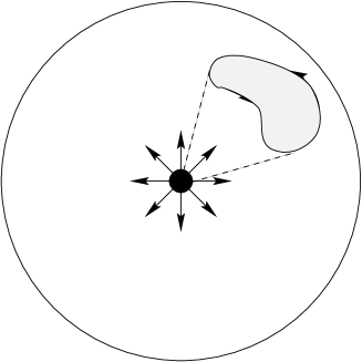
Figure 1.25: Magnetic monopole in spin space. Arrows indicate the curl of the Berry connection $\vec{\nabla}\times\vec{\mathcal{A}}$ emanating from the origin. Shaded region indicates closed path $\vec{m}(t)$ taken by the spin order parameter during which it acquires a Berry phase proportional to the monopole flux passing through the shaded region.

Recalling eq. (1.20), we see that the Lagrangian for a single spin in eq. (1.216) is equivalent to the Lagrangian of a massless object of charge $-S$, located at position $\vec{m}$, moving on the unit sphere containing a magnetic monopole. The Zeeman term represents a constant electric field $-\vec{\Delta}$ producing a force $\vec{\Delta}S$ on the particle. The Lorentz force caused by the monopole causes the particle to orbit the sphere at constant ‘latitude’. Because no kinetic term of the form $\dot{m}^{\alpha}\dot{m}^{\alpha}$ enters the Lagrangian, the charged particle is massless and so lies only in the lowest Landau level of the monopole field. Note the similarity here to the previous discussion of the high field limit and the semiclassical percolation picture of the integer Hall effect. For further details the reader is directed to appendix B and to Haldane’s discussion of monopole spherical harmonics [48].

If the ‘charge’ moves slowly around a closed counterclockwise path $\vec{m}(t)$ during the time interval $[0,T]$ as illustrated in fig. (1.25), the quantum amplitude

$$e^{\frac{i}{\hbar}\int_{0}^{T}dt\mathcal{L}}$$ (1.227)

contains a Berry’s phase [49] contribution proportional to the ‘magnetic flux’ enclosed by the path

$$e^{-iS\int_{0}^{T}dt\dot{m}^{\nu}\mathcal{A}^{\nu}}=e^{-iS\oint\vec{\mathcal{A}}\cdot d\vec{m}}.$$ (1.228)

As discussed in appendix B, this is a purely geometric phase in the sense that it depends only on the geometry of the path and not the rate at which the path is traversed (since the expression is time reparameterization invariant). Using Stokes theorem and eq. (1.226) we can write the contour integral as a surface integral

$$e^{-iS\oint\vec{\mathcal{A}}\cdot d\vec{m}}=e^{-iS\int d\vec{\Omega}\cdot\vec{\nabla}\times\vec{\mathcal{A}}}=e^{-iS\Omega}$$ (1.229)

where $d\vec{\Omega}=\vec{m}d\Omega$ is the directed area (solid angle) element and $\Omega$ is the total solid angle subtended by the contour as viewed from the position of the monopole. Note from fig. (1.25) that there is an ambiguity on the sphere as to which is the inside and which is the outside of the contour. Since the total solid angle is $4\pi$ we could equally well have obtained

$$e^{+iS(4\pi-\Omega)}.$$ (1.230)

Thus the phase is ambiguous unless $S$ is an integer or half-integer. This constitutes a ‘proof’ that the quantum spin length must be quantized.

Having obtained the correct Lagrangian for our toy model we can now readily generalize it to the spin wave problem using the potential energy in eq. (1.214)

$$\mathcal{L} = -\hbar Sn\int d^{2}r\;\Biggl{\{}\dot{m}^{\mu}(\vec{r}\,)\;\mathcal{A}^{\mu}[\vec{m}]-\Delta m^{z}(\vec{r}\,)\Biggr{\}}$$ (1.231)

$$-\frac{1}{2}\rho_{s}\int d^{2}r\;\partial_{\mu}m^{\nu}\partial_{\mu}m^{\nu}+\int d^{2}r\;\lambda(\vec{r}\,)\;(m^{\mu}m^{\mu}-1).$$

The classical equation of motion can be analyzed just as for the toy model, however we will take a slightly different approach here. Let us look in the low energy sector where the spins all lie close to the $\hat{z}$ direction. Then we can write

$$\vec{m} = \left(m^{x},m^{y},\sqrt{1-m^{x}m^{x}-m^{y}m^{y}}\right)$$ (1.232)

$$\approx \left(m^{x},m^{y},1-\frac{1}{2}m^{x}m^{x}-\frac{1}{2}m^{y}m^{y}\right).$$

Now choose the ‘symmetric gauge’

$$\vec{\mathcal{A}}\approx\frac{1}{2}(-m^{y},m^{x},0)$$ (1.233)

which obeys eq. (1.226) for $\vec{m}$ close to $\hat{z}$.

Keeping only quadratic terms in the Lagrangian we obtain

$$\mathcal{L} = -\hbar Sn\int d^{2}r\;\bigg{\{}\frac{1}{2}(\dot{m}^{y}m^{x}-\dot{m}^{x}m^{y})$$ (1.234)

$$-\Delta\left(1-\frac{1}{2}m^{x}m^{x}-\frac{1}{2}m^{y}m^{y}\right)\bigg{\}}$$

$$-\frac{1}{2}\rho_{s}\int d^{2}r\;(\partial_{\mu}m^{x}\partial_{\mu}m^{x}+\partial_{\mu}m^{y}\partial_{\mu}m^{y}).$$

This can be conveniently rewritten by defining a complex field

$$\psi\equiv m^{x}+im^{y}$$

$$\mathcal{L} = -Sn\hbar\int d^{2}r\;\bigg{\{}\frac{1}{4}\left[\psi^{*}\left(-i\frac{\partial}{\partial t}\right)\psi-\psi\left(-i\frac{\partial}{\partial t}\right)\psi^{*}\right]$$ (1.235)

$$-\Delta\left(1-\frac{1}{2}\psi^{*}\psi\right)\bigg{\}}-\frac{1}{2}\rho_{s}\int d^{2}r\;\partial_{\mu}\psi^{*}\partial_{\mu}\psi$$

The classical equation of motion is the Schrödinger like equation

$$+i\hbar\frac{\partial\psi}{\partial t}=-\frac{\rho_{s}}{nS}\partial_{\mu}^{2}\psi+\hbar\Delta\psi.$$ (1.236)

This has plane wave solutions with quantum energy

$$\epsilon_{k}=\hbar\Delta+\frac{\rho_{s}}{nS}k^{2}.$$ (1.237)

We can fit the phenomenological stiffness to the exact dispersion relation in eq. (1.209) to obtain

$$\rho_{s}=\frac{nS}{4}\sum_{k\neq 0}e^{-\frac{1}{2}|k|^{2}}\;v(k)|k|^{2}.$$ (1.238)

Exercise 1.20

Derive eq. (1.238) from first principles by evaluating the loss of exchange energy when the Landau gauge $\nu=1$ ground state is distorted to make the spin tumble in the $x$ direction $$|\psi\rangle=\prod_{k}\left(\cos{\frac{\theta_{k}}{2}}c_{k\uparrow}^{\dagger}+\sin{\frac{\theta_{k}}{2}}c_{k\downarrow}^{\dagger}\right)|0\rangle$$ (1.239) where $\theta_{k}=-\gamma k\ell^{2}$ and $\gamma=\frac{\partial\theta}{\partial x}$ is the (constant) spin rotation angle gradient (since $x=-k\ell^{2}$ in this gauge).

1.10.5 Topological Excitations

So far we have studied neutral collective excitations that take the form of spin waves. They are neutral because as we have seen from eq. (1.204) they consist of a particle-hole pair. For very large momenta the spin-flipped particle is translated a large distance $\vec{q}\times\hat{z}\ell^{2}$ away from its original position as discussed in appendix A. This looks locally like a charged excitation but it is very expensive because it loses all of its exchange energy. It is sensible to inquire if it is possible to make a cheaper charged excitation. This can indeed be done by taking into account the desire of the spins to be locally parallel and producing a smooth topological defect in the spin orientation [50, 46, 51, 52, 53, 54, 55, 56] known as a skyrmion by analogy with related objects in the Skyrme model of nuclear physics [57]. Such an object has the beautiful form exhibited in fig. (1.26).

Figure 1.26: Illustration of a skyrmion spin texture. The spin is down at the origin and gradually turns up at infinite radius. At intermediate distances, the XY components of the spin exhibit a vortex-like winding. Unlike a $U(1)$ vortex, there is no singularity at the origin.

Rather than having a single spin suddenly flip over, this object gradually turns over the spins as the center is approached. At intermediate distances the spins have a vortex-like configuration. However unlike a $U(1)$ vortex, there is no singularity in the core region because the spins are able to rotate downwards out of the xy plane.

In nuclear physics the Skyrme model envisions that the vacuum is a ‘ferromagnet’ described by a four component field $\Phi^{\mu}$ subject to the constraint $\Phi^{\mu}\Phi^{\mu}=1$. There are three massless (i.e. linearly dispersing) spin wave excitations corresponding to the three directions of oscillation about the ordered direction. These three massless modes represent the three (nearly) massless pions $\pi^{+},\pi^{0},\pi^{-}$. The nucleons (proton and neutron) are represented by skyrmion spin textures. Remarkably, it can be shown (for an appropriate form of the action) that these objects are fermions despite the fact that they are in a sense made up of a coherent superposition of (an infinite number of) bosonic spin waves.

We shall see a very similar phenomenology in QHE ferromagnets. At filling factor $\nu$, skyrmions have charge $\pm\nu e$ and fractional statistics much like Laughlin quasiparticles. For $\nu=1$ these objects are fermions. Unlike Laughlin quasiparticles, skyrmions are extended objects, and they involve many flipped (and partially flipped) spins. This property has profound implications as we shall see.

Let us begin our analysis by understanding how it is that spin textures can carry charge. It is clear from the Pauli principle that it is necessary to flip at least some spins to locally increase the charge density in a $\nu=1$ ferromagnet. What is the sufficient condition on the spin distortions in order to have a density fluctuation? Remarkably it turns out to be possible, as we shall see, to uniquely express the charge density solely in terms of gradients of the local spin orientation.

Consider a ferromagnet with local spin orientation $\vec{m}(\vec{r}\,)$ which is static. As each electron travels we assume that the strong exchange field keeps the spin following the local orientation $\vec{m}$. If the electron has velocity $\dot{x}^{\mu}$, the rate of change of the local spin orientation it sees is $\dot{m}^{\nu}=\dot{x}^{\mu}\frac{\partial}{\partial x^{\mu}}m^{\nu}$. This in turn induces an additional Berry’s phase as the spin orientation varies. Thus the single-particle Lagrangian contains an additional first order time derivative in addition to the one induced by the magnetic field coupling to the orbital motion

$$\mathcal{L}_{0}=-\frac{e}{c}\dot{x}^{\mu}A^{\mu}+\hbar S\dot{m}^{\nu}\mathcal{A}^{\nu}[\vec{m}].$$ (1.240)

Here $A^{\mu}$ refers to the electromagnetic vector potential and $\mathcal{A}^{\nu}$ refers to the monopole vector potential obeying eq. (1.226) and we have set the mass to zero (i.e. dropped the $\frac{1}{2}M\;\dot{x}^{\mu}\dot{x}^{\mu}$ term). This can be rewritten

$$\mathcal{L}_{0}=-\frac{e}{c}\dot{x}^{\mu}(A^{\mu}+a^{\mu})$$ (1.241)

where (with $\Phi_{0}$ being the flux quantum)

$$a^{\mu}\equiv-\Phi_{0}S\left(\frac{\partial}{\partial x^{\mu}}m^{\nu}\right)\;\mathcal{A}^{\nu}[\vec{m}]$$ (1.242)

represents the ‘Berry connection’, an additional vector potential which reproduces the Berry phase. The additional fake magnetic flux due to the curl of the Berry connection is

$$b = \epsilon^{\alpha\beta}\frac{\partial}{\partial x^{\alpha}}a^{\beta}$$ (1.243)

$$= -\Phi_{0}S\epsilon^{\alpha\beta}\frac{\partial}{\partial x^{\alpha}}\;\left(\frac{\partial}{\partial x^{\beta}}m^{\nu}\right)\mathcal{A}^{\nu}[\vec{m}]$$

$$= -\Phi_{0}S\epsilon^{\alpha\beta}\left\{\left(\frac{\partial}{\partial x^{\alpha}}\;\frac{\partial}{\partial x^{\beta}}m^{\nu}\right)\mathcal{A}^{\nu}[\vec{m}]\right.$$

$$\left.+\left(\frac{\partial}{\partial x^{\beta}}m^{\nu}\right)\;\frac{\partial m^{\gamma}}{\partial x^{\alpha}}\;\frac{\partial\mathcal{A}^{\nu}}{\partial m^{\gamma}}\right\}.$$

The first term vanishes by symmetry leaving

$$b=-\Phi_{0}S\epsilon^{\alpha\beta}\frac{\partial m^{\nu}}{\partial x^{\beta}}\;\frac{\partial m^{\gamma}}{\partial x^{\alpha}}\;\frac{1}{2}F^{\nu\gamma}$$ (1.244)

where $F^{\nu\gamma}$ is given by eq. (1.222) and we have taken advantage of the fact that the remaining factors are antisymmetric under the exchange $\nu\leftrightarrow\gamma$. Using eq. (1.222) and setting $S=\frac{1}{2}$ we obtain

$$b=-\Phi_{0}\tilde{\rho}$$ (1.245)

where

$$\tilde{\rho} \equiv \frac{1}{8\pi}\epsilon^{\alpha\beta}\epsilon^{abc}m^{a}\partial_{\alpha}m^{b}\partial_{\beta}m^{c}$$ (1.246)

$$= \frac{1}{8\pi}\epsilon^{\alpha\beta}\vec{m}\cdot\partial_{\alpha}\vec{m}\times\partial_{\beta}\vec{m}$$

is (for reasons that will become clear shortly) called the topological density or the Pontryagin density.

Imagine now that we adiabatically deform the uniformly magnetized spin state into some spin texture state. We see from eq. (1.245) that the orbital degrees of freedom see this as adiabatically adding additional flux $b(\vec{r}\,)$. Recall from eq. (1.178) and the discussion of the charge of the Laughlin quasiparticle, that extra charge density is associated with extra flux in the amount

$$\delta\rho = \frac{1}{c}\sigma_{xy}b$$ (1.247)

$$\delta\rho = \nu e\tilde{\rho}.$$ (1.248)

Thus we have the remarkable result that the changes in the electron charge density are proportional to the topological density.

Our assumption of adiabaticity is valid as long as the spin fluctuation frequency is much lower than the charge excitation gap. This is an excellent approximation for $\nu=1$ and still good on the stronger fractional Hall plateaus.

It is interesting that the fermionic charge density in this model can be expressed solely in terms of the vector boson field $\vec{m}(\vec{r}\,)$, but there is something even more significant here. The skyrmion spin texture has total topological charge

$$Q_{\mathrm{top}}\equiv\frac{1}{8\pi}\int d^{2}r\;\epsilon^{\alpha\beta}\vec{m}\cdot\partial_{\alpha}\vec{m}\times\partial_{\beta}\vec{m}$$ (1.249)

which is always an integer. In fact for any smooth spin texture in which the spins at infinity are all parallel, $Q_{\mathrm{top}}$ is always an integer. Since it is impossible to continuously deform one integer into another, $Q_{\mathrm{top}}$ is a topological invariant. That is, if $Q_{\mathrm{top}}=\pm 1$ because a skyrmion (anti-skyrmion) is present, $Q_{\mathrm{top}}$ is stable against smooth continuous distortions of the field $\vec{m}$. For example a spin wave could pass through the skyrmion and $Q_{\mathrm{top}}$ would remain invariant. Thus this charged object is topologically stable and has fermion number (i.e., the number of fermions (electrons) that flow into the region when the object is formed)

$$N=\nu Q_{\mathrm{top}}.$$ (1.250)

For $\nu=1$, $N$ is an integer ($\pm 1$ say) and has the fermion number of an electron. It is thus continuously connected to the single flipped spin example discussed earlier.

We are thus led to the remarkable conclusion that the spin degree of freedom couples to the electrostatic potential. Because skyrmions carry charge, we can affect the spin configuration using electric rather than magnetic fields!

To understand how $Q_{\mathrm{top}}$ always turns out to be an integer, it is useful to consider a simpler case of a one-dimensional ring. We follow here the discussion of [58]. Consider the unit circle (known to topologists as the one-dimensional sphere $S_{1}$). Let the angle $\theta\;\epsilon[0,2\pi]$ parameterize the position along the curve. Consider a continuous, suitably well-behaved, complex function $\psi(\theta)=e^{i\varphi(\theta)}$ defined at each point on the circle and obeying $|\psi|=1$. Thus associated with each point $\theta$ is another unit circle giving the possible range of values of $\psi(\theta)$. The function $\psi(\theta)$ thus defines a trajectory on the torus $S_{1}\times S_{1}$ illustrated in fig. (1.27).

Figure 1.27: Illustration of mappings $\varphi(\theta)$ with: zero winding number (left) and winding number $+2$ (right).

The possible functions $\psi(\theta)$ can be classified into different homotopy classes according to their winding number $n\in\mathbf{Z}$

$$n \equiv \frac{1}{2\pi}\int_{0}^{2\pi}d\theta\;\psi^{*}\left(-i\frac{d}{d\theta}\right)\psi$$ (1.251)

$$= \frac{1}{2\pi}\int_{0}^{2\pi}d\theta\;\frac{d\varphi}{d\theta}=\frac{1}{2\pi}\left[\varphi(2\pi)-\varphi(0)\right].$$

Because the points $\theta=0$ and $\theta=2\pi$ are identified as the same point

$$\psi(0)=\psi(2\pi)\Rightarrow\varphi(2\pi)-\varphi(0)=2\pi\times\mbox{ integer}$$ (1.252)

and so $n$ is an integer. Notice the crucial role played by the fact that the ‘topological density’ $\frac{1}{2\pi}\;\frac{d\varphi}{d\theta}$ is the Jacobian for converting from the coordinate $\theta$ in the domain to the coordinate $\varphi$ in the range. It is this fact that makes the integral in eq. (1.251) independent of the detailed local form of the mapping $\varphi(\theta)$ and depend only on the overall winding number. As we shall shortly see, this same feature will also turn out to be true for the Pontryagin density.

Think of the function $\varphi(\theta)$ as defining the path of an elastic band wrapped around the torus. Clearly the band can be stretched, pulled and distorted in any smooth way without any effect on $n$. The only way to change the winding number from one integer to another is to discontinuously break the elastic band, unwind (or wind) some extra turns, and then rejoin the cut pieces.

Another way to visualize the homotopy properties of mappings from $S_{1}$ to $S_{1}$ is illustrated in fig. (1.28).

Figure 1.28: A different representation of the mappings from $\theta$ to $\varphi$. The dashed line represents the domain $\theta$ and the solid line represents the range $\varphi$. The domain is ‘lifted up’ by the mapping and placed on the range. The winding number $n$ is the number of times the dashed circle wraps the solid circle (with a possible minus sign depending on the orientation).

The solid circle represents the domain $\theta$ and the dashed circle represents the range $\varphi$. It is useful to imagine the $\theta$ circle as being an elastic band (with points on it labeled by coordinates running from $0$ to $2\pi$) which can be ‘lifted up’ to the $\varphi$ circle in such a way that each point of $\theta$ lies just outside the image point $\varphi(\theta)$. The figure illustrates how the winding number $n$ can be interpreted as the number of times the domain $\theta$ circle wraps around the range $\varphi$ circle. (Note: even though the elastic band is ‘stretched’ and may wrap around the $\varphi$ circle more than once, its coordinate labels still only run from $0$ to $2\pi$.) This interpretation is the one which we will generalize for the case of skyrmions in 2D ferromagnets.

We can think of the equivalence class of mappings having a given winding number as an element of a group called the homotopy group $\pi_{1}(S_{1})$. The group operation is addition and the winding number of the sum of two functions, $\varphi(\theta)\equiv\varphi_{1}(\theta)+\varphi_{2}(\theta)$, is the sum of the two winding numbers $n=n_{1}+n_{2}$. Thus $\pi_{1}(S_{1})$ is isomorphic to $\mathbf{Z}$, the group of integers under addition.

Returning now to the ferromagnet we see that the unit vector order parameter $\vec{m}$ defines a mapping from the plane $R_{2}$ to the two-sphere $S_{2}$ (i.e. an ordinary sphere in three dimensions having a two-dimensional surface). Because we assume that $\vec{m}=\hat{z}$ for all spatial points far from the location of the skyrmion, we can safely use a projective map to ‘compactify’ $R_{2}$ into a sphere $S_{2}$. In this process all points at infinity in $R_{2}$ are mapped into a single point on $S_{2}$, but since $\vec{m}(\vec{r})$ is the same for all these different points, no harm is done. We are thus interested in the generalization of the concept of the winding number to the mapping $S_{2}\rightarrow S_{2}$. The corresponding homotopy group $\pi_{2}(S_{2})$ is also equivalent to $\mathbf{Z}$ as we shall see.

Consider the following four points in the plane and their images (illustrated in fig. (1.29)) under the mapping

$$(x,y) \longrightarrow \vec{m}(x,y)$$

$$(x+dx,y) \longrightarrow \vec{m}(x+dx,y)$$

$$(x,y+dy) \longrightarrow \vec{m}(x,y+dy)$$

$$(x+dx,y+dy) \longrightarrow \vec{m}(x+dx,y+dy).$$ (1.253)

The four points in the plane define a rectangle of area $dxdy$. The four points on the order parameter (spin) sphere define an approximate parallelogram whose area (solid angle) is

$$d\omega \approx \left[\vec{m}(x+dx,y)-\vec{m}(x,y)\right]\times\left[\vec{m}(x,y+dy)-\vec{m}(x,y)\right]\cdot\vec{m}(x,y)$$ (1.254)

$$\approx \frac{1}{2}\epsilon^{\mu\nu}\;\vec{m}\cdot\partial_{\mu}\vec{m}\times\partial_{\nu}\vec{m}\;dxdy$$

$$= 4\pi\tilde{\rho}\;dxdy.$$

Thus the Jacobian converting area in the plane into solid angle on the sphere is $4\pi$ times the Pontryagin density $\tilde{\rho}$. This means that the total topological charge given in eq. (1.249) must be an integer since it counts the number of times the compactified plane is wrapped around the order parameter sphere by the mapping. The ‘wrapping’ is done by lifting each point $\vec{r}$ in the compactified plane up to the corresponding point $\vec{m}(\vec{r}\,)$ on the sphere just as was described for $\pi_{1}(S_{1})$ in fig. (1.28).

Figure 1.29: Infinitesimal circuit in spin space associated with an infinitesimal circuit in real space via the mapping $\vec{m}(\vec{r})$.

For the skyrmion illustrated in fig. (1.26) the order parameter function $\vec{m}(\vec{r}\,)$ was chosen to be the standard form that minimizes the gradient energy [58]

$$m^{x} = \frac{2\lambda r\;\cos{(\theta-\varphi)}}{\lambda^{2}+r^{2}}$$ (1.255a)

$$m^{y} = \frac{2\lambda r\;\sin{(\theta-\varphi)}}{\lambda^{2}+r^{2}}$$ (1.255b)

$$m^{z} = \frac{r^{2}-\lambda^{2}}{\lambda^{2}+r^{2}}$$ (1.255c)

where $(r,\theta)$ are the polar coordinates in the plane, $\lambda$ is a constant that controls the size scale, and $\varphi$ is a constant that controls the XY spin orientation. (Rotations about the Zeeman axis leave the energy invariant.) From the figure it is not hard to see that the skyrmion mapping wraps the compactified plane around the order parameter sphere exactly once. The sense is such that $Q_{\mathrm{top}}=-1$.

Exercise 1.21

Show that the topological density can be written in polar spatial coordinates as $$\tilde{\rho}=\frac{1}{4\pi r}\vec{m}\cdot\frac{\partial\vec{m}}{\partial r}\times\frac{\partial\vec{m}}{\partial\theta}.$$ Use this result to show $$\tilde{\rho}=-\frac{1}{4\pi}\left(\frac{2\lambda}{\lambda^{2}+r^{2}}\right)^{2}$$ and hence $$Q_{\mathrm{top}}=-1$$ for the skyrmion mapping in eqs. (1.255a–1.255c).

It is worthwhile to note that it is possible to write down simple microscopic variational wave functions for the skyrmion which are closely related to the continuum field theory results obtained above. Consider the following state in the plane [51]

$$\psi_{\lambda}=\prod_{j}\left(\begin{array}[]{c}z_{j}\\ \lambda\end{array}\right)_{j}\Psi_{1},$$ (1.256)

where $\Psi_{1}$ is the $\nu=1$ filled Landau level state $(\cdot)_{j}$ refers to the spinor for the $j$th particle, and $\lambda$ is a fixed length scale. This is a skyrmion because it has its spin purely down at the origin (where $z_{j}=0$) and has spin purely up at infinity (where $|z_{j}|\gg\lambda$). The parameter $\lambda$ is simply the size scale of the skyrmion [46, 58]. At radius $\lambda$ the spinor has equal weight for up and down spin states (since $|z_{j}|=\lambda$) and hence the spin lies in the XY plane just as it does for the solution in eq. (1.255c). Notice that in the limit $\lambda\longrightarrow 0$ (where the continuum effective action is invalid but this microscopic wave function is still sensible) we recover a fully spin polarized filled Landau level with a charge-1 Laughlin quasihole at the origin. Hence the number of flipped spins interpolates continuously from zero to infinity as $\lambda$ increases.

In order to analyze the skyrmion wave function in eq. (1.256), we use the Laughlin plasma analogy. Recall from our discussion in sec. 1.6.1 that in this analogy the norm of $\psi_{\lambda}$, $Tr_{\{\sigma\}}\int D[z]\;|\Psi[z]|^{2}$ is viewed as the partition function of a Coulomb gas. In order to compute the density distribution we simply need to take a trace over the spin

$$Z=\int D[z]\;e^{-2\left\{\sum_{i>j}-\log{|z_{i}-z_{j}|}-\frac{1}{2}\sum_{k}\log{(|z_{k}|^{2}+\lambda^{2})}+\frac{1}{4}\sum_{k}|z_{k}|^{2}\right\}}.$$ (1.257)

This partition function describes the usual logarithmically interacting Coulomb gas with uniform background charge plus a spatially varying impurity background charge $\Delta\rho_{b}(r)$,

$$\Delta\rho_{b}(r) \equiv -\frac{1}{2\pi}\nabla^{2}V(r)=+\frac{\lambda^{2}}{\pi(r^{2}+\lambda^{2})^{2}},$$ (1.258)

$$V(r) = -\frac{1}{2}\log{(r^{2}+\lambda^{2})}.$$ (1.259)

For large enough scale size $\lambda\gg\ell$, local neutrality of the plasma [59] forces the electrons to be expelled from the vicinity of the origin and implies that the excess electron number density is precisely $-\Delta\rho_{b}(r)$, so that eq. (1.258) is in agreement with the standard result [58] for the topological density given in ex. 1.21.

Just as it was easy to find an explicit wave function for the Laughlin quasi-hole but proved difficult to write down an analytic wave function for the Laughlin quasi-electron, it is similarly difficult to make an explicit wave function for the anti-skyrmion. Finally, we note that by replacing $z\choose\lambda$ by $z^{n}\choose\lambda^{n}$, we can generate a skyrmion with a Pontryagin index $n$.

Exercise 1.22

The argument given above for the charge density of the microscopic skyrmion state wave function used local neutrality of the plasma and hence is valid only on large length scales and thus requires $\lambda\gg\ell$. Find the complete microscopic analytic solution for the charge density valid for arbitrary $\lambda$, by using the fact that the proposed manybody wave function is nothing but a Slater determinant of the single particle states $\phi_{m}(z)$, $$\phi_{m}(z)=\frac{z^{m}}{\sqrt{2\pi 2^{m+1}m!\left(m+1+\frac{\lambda^{2}}{2}\right)}}{z\choose\lambda}e^{-\frac{|z^{2}|}{4}}.$$ (1.260) Show that the excess electron number density is then $$\Delta n^{(1)}(z)\equiv\sum_{m=0}^{N-1}|\phi_{m}(z)|^{2}-\frac{1}{2\pi},$$ (1.261) which yields $$\Delta n^{(1)}(z)=\frac{1}{2\pi}\left(\frac{1}{2}\int_{0}^{1}d\alpha\;\alpha^{\frac{\lambda^{2}}{2}}e^{-\frac{|z|^{2}}{2}(1-\alpha)}(|z|^{2}+\lambda^{2})-1\right).$$ (1.262) Similarly, find the spin density distribution $S^{z}(r)$ and show that it also agrees with the field-theoretic expression in eq. (1.255c) in the large $\lambda$ limit.

The skyrmion solution in eqs. (1.255a–1.255c) minimizes the gradient energy

$$E_{0}=\frac{1}{2}\rho_{s}\int d^{2}r\;\partial_{\mu}m^{\nu}\partial_{\mu}m^{\nu}.$$ (1.263)

Notice that the energy cost is scale invariant since this expression contains two integrals and two derivatives. Hence the total gradient energy is independent of the scale factor $\lambda$ and for a single skyrmion is given by [46, 58]

$$E_{0}=4\pi\rho_{s}=\frac{1}{4}\epsilon_{\infty}$$ (1.264)

where $\epsilon_{\infty}$ is the asymptotic large $q$ limit of the spin wave energy in eq. (1.208). Since this spin wave excitation produces a widely separated particle-hole pair, we see that the energy of a widely separated skyrmion-antiskyrmion pair $\left(\frac{1}{4}+\frac{1}{4}\right)\epsilon_{\infty}$ is only half as large. Thus skyrmions are considerably cheaper to create than simple flipped spins.

Notice that eq. (1.264) tells us that the charge excitation gap, while only half as large as naively expected, is finite as long as the spin stiffness $\rho_{s}$ is finite. Thus we can expect a dissipationless Hall plateau. Therefore, as emphasized by Sondhi et al. [46], the Coulomb interaction plays a central role in the $\nu=1$ integer Hall effect. Without the Coulomb interaction the charge gap would simply be the tiny Zeeman gap. With the Coulomb interaction the gap is large even in the limit of zero Zeeman energy because of the spontaneous ferromagnetic order induced by the spin stiffness.

At precisely $\nu=1$ skyrmion/antiskyrmion pairs will be thermally activated and hence exponentially rare at low temperatures. On the other hand, because they are the cheapest way to inject charge into the system, there will be a finite density of skyrmions even in the ground state if $\nu\neq 1$. Skyrmions also occur in ordinary 2D magnetic films but since they do not carry charge (and are energetically expensive since $\rho_{s}$ is quite large) they readily freeze out and are not particularly important.

The charge of a skyrmion is sharply quantized but its number of flipped spins depends on its area $\sim\lambda^{2}$. Hence if the energy were truly scale invariant, the number of flipped spins could take on any value. Indeed one of the early theoretical motivations for skyrmions was the discovery in numerical work by Rezayi [46, 60] that adding a single charge to a filled Landau level converted the maximally ferromagnetic state into a spin singlet. In the presence of a finite Zeeman energy the scale invariance is lost and there is a term in the energy that scales with $\Delta\lambda^{2}$ and tries to minimize the size of the skyrmion. Competing with this however is a Coulomb term which we now discuss.

The Lagrangian in eq. (1.231) contains the correct leading order terms in a gradient expansion. There are several possible terms which are fourth order in gradients, but a particular one dominates over the others at long distances. This is the Hartree energy associated with the charge density of the skyrmion

$$V_{\mathrm{H}}=\frac{1}{2\epsilon}\int d^{2}r\;\int d^{2}r^{\prime}\;\frac{\delta\rho(\vec{r}\,)\;\delta\rho(\vec{r}^{\,\prime})}{|\vec{r}-\vec{r}^{\,\prime}|}$$ (1.265)

where

$$\delta\rho=\frac{\nu e}{8\pi}\;\epsilon^{\alpha\beta}\;\vec{m}\cdot\partial_{\alpha}\vec{m}\times\partial_{\beta}\vec{m}$$ (1.266)

and $\epsilon$ is the dielectric constant. The long range of the Coulomb interaction makes this effectively a three gradient term that distinguishes it from the other possible terms at this order. Recall that the Coulomb interaction already entered in lower order in the computation of $\rho_{s}$. That however was the exchange energy while the present term is the Hartree energy. The Hartree energy scales like $\frac{e^{2}}{\epsilon\lambda}$ and so prefers to expand the skyrmion size. The competition between the Coulomb and Zeeman energies yields an optimal number of approximately four flipped spins according to microscopic Hartree Fock calculations [61].

Thus a significant prediction for this model is that each charge added (or removed) from a filled Landau level will flip several $(\sim 4)$ spins. This is very different from what is expected for non-interacting electrons. As illustrated in fig. (1.30)

Figure 1.30: Illustration of the spin configurations for non-interacting electrons at filling factor $\nu=1$ in the presence of a hole (top) and an extra electron (bottom).

removing an electron leaves the non-interacting system still polarized. The Pauli principle forces an added electron to be spin reversed and the magnetization drops from unity at $\nu=1$ to zero at $\nu=2$ where both spin states of the lowest Landau level are fully occupied.

Direct experimental evidence for the existence of skyrmions was first obtained by Barrett et al. [62] using a novel optically pumped NMR technique. The Hamiltonian for a nucleus is [63]

$$H_{N}=-\Delta_{N}I^{z}+\Omega\vec{I}\cdot\vec{s}$$ (1.267)

where $\vec{I}$ is the nuclear angular momentum, $\Delta_{N}$ is the nuclear Zeeman frequency (about 3 orders of magnitude smaller than the electron Zeeman frequency), $\Omega$ is the hyperfine coupling and $\vec{s}$ is the electron spin density at the nuclear site. If, as a first approximation we replace $\vec{s}$ by its average value

$$H_{N}\approx\left(-\Delta_{N}+\Omega\langle s^{z}\rangle\right)\;I^{z}$$ (1.268)

we see that the precession frequency of the nucleus will be shifted by an amount proportional to the magnetization of the electron gas. The magnetization deduced using this so-called Knight shift is shown in fig. (1.31).

Figure 1.31: NMR Knight shift measurement of the electron spin polarization near filling factor $\nu=1$. Circles are the data of Barrett et al. [62]. The dashed line is a guide to the eye. The solid line is the prediction for non-interacting electrons. The peak represents 100% polarization at $\nu=1$. The steep slope on each side indicates that many ($\sim 4$) spins flip over for each charge added (or subtracted). The observed symmetry around $\nu=1$ is due to the particle-hole symmetry between skyrmions and antiskyrmions not present in the free-electron model.

The electron gas is 100% polarized at $\nu=1$, but the polarization drops off sharply (and symmetrically) as charge is added or subtracted. This is in sharp disagreement with the prediction of the free electron model as shown in the figure. The initial steep slope of the data allows one to deduce that 3.5–4 spins reverse for each charge added or removed. This is in excellent quantitative agreement with Hartree-Fock calculations for the skyrmion model [61].

Other evidence for skyrmions comes from the large change in Zeeman energy with field due to the large number of flipped spins. This has been observed in transport [64] and in optical spectroscopy [65]. Recall that spin-orbit effects in GaAs make the electron $g$ factor $-0.4$. Under hydrostatic pressure $g$ can be tuned towards zero which should greatly enhance the skyrmion size. Evidence for this effect has been seen [66].

1.11 Skyrmion Dynamics

NMR [62] and nuclear specific heat [67] data indicate that skyrmions dramatically enhance the rate at which the nuclear spins relax. This nuclear spin relaxation is due to the transverse terms in the hyperfine interaction which we neglected in discussing the Knight shift

$$\frac{1}{2}\Omega\;(I^{+}s^{-}+I^{-}s^{+})=\frac{1}{2}\Omega\;\left\{I^{+}\sum_{\vec{q}}S_{\vec{q}}^{-}+\mbox{h.c.}\right\}.$$ (1.269)

The free electron model would predict that it would be impossible for an electron and a nucleus to undergo mutual spin flips because the Zeeman energy would not be conserved. (Recall that $\Delta_{N}\sim 10^{-3}\Delta$.) The spin wave model shows that the problem is even worse than this. Recall from eq. (1.208) that the spin Coulomb interaction makes spin wave energy much larger than the electron Zeeman gap except at very long wavelengths. The lowest frequency spin wave excitations lie above 20–50 GHz while the nuclei precess at 10–100 MHz. Hence the two sets of spins are unable to couple effectively. At $\nu=1$ this simple picture is correct. The nuclear relaxation time $T_{1}$ is extremely long (tens of minutes to many hours depending on the temperature) as shown in fig. (1.32).

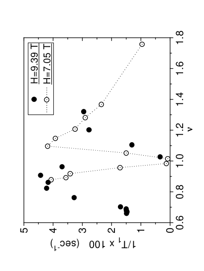
Figure 1.32: NMR nuclear spin relaxation rate $1/T_{1}$ as a function of filling factor. After Tycko et al. [68]. The relaxation rate is very small at $\nu=1$, but rises dramatically away from $\nu=1$ due to the presence of skyrmions.

However the figure also shows that for $\nu\neq 1$ the relaxation rate $1/T_{1}$ rises dramatically and $T_{1}$ falls to $\sim 20~{}\mbox{seconds}$. In order to understand this dramatic variation we need to develop a theory of spin dynamics in the presence of skyrmions.

The $1/T_{1}$ data is telling us that for $\nu\neq 1$ at least some of the electron spin fluctuations are orders of magnitude lower in frequency than the Zeeman splitting and these low frequency modes can couple strongly to the nuclei. One way this might occur is through the presence of disorder. We see from eq. (1.269) that NMR is a local probe which couples to spin flip excitations at all wave vectors. Recall from eq. (1.204) that lowest Landau level projection implies that $\overline{S_{\vec{q}}^{-}}$ contains a translation operator $\tau_{q}$. In the presence of strong disorder the Zeeman and exchange cost of the spin flips could be compensated by translation to a region of lower potential energy. Such a mechanism was studied in [69] but does not show sharp features in $1/T_{1}$ around $\nu=1$.

We are left only with the possibility that the dynamics of skyrmions somehow involves low frequency spin fluctuations. For simplicity we will analyze this possibility ignoring the effects of disorder, although this may not be a valid approximation.

Let us begin by considering a ferromagnetic $\nu=1$ state containing a single skyrmion of the form parameterized in eqs. (1.255a–1.255c). There are two degeneracies at the classical level in the effective field theory: The energy does not depend on the position of the skyrmion and it does not depend on the angular orientation $\varphi$. These continuous degeneracies are known as zero modes [58] and require special treatment of the quantum fluctuations about the classical solution.

In the presence of one or more skyrmions, the quantum Hall ferromagnet is non-colinear. In an ordinary ferromagnet where all the spins are parallel, global rotations about the magnetization axis only change the quantum phase of the state — they do not produce a new state. Because the skyrmion has distinguishable orientation, each one induces a new $U(1)$ degree of freedom in the system. In addition because the skyrmion has a distinguishable location, each one induces a new translation degree of freedom. As noted above, both of these are zero energy modes at the classical level suggesting that they might well be the source of low energy excitations which couple so effectively to the nuclei. We shall see that this is indeed the case, although the story is somewhat complicated by the necessity of correctly quantizing these modes.

Let us begin by finding the effective Lagrangian for the translation mode [8]. We take the spin configuration to be

$$\vec{m}(\vec{r},t)=\vec{m}_{0}\left(\vec{r}-\vec{R}(t)\right)$$ (1.270)

where $\vec{m}_{0}$ is the static classical skyrmion solution and $\vec{R}(t)$ is the position degree of freedom. We ignore all other spin wave degrees of freedom since they are gapped. (The gapless $U(1)$ rotation mode will be treated separately below.) Eq. (1.231) yields a Berry phase term

$$\mathcal{L}_{0}=-\hbar S\int d^{2}r\;\dot{m}^{\mu}\mathcal{A}^{\mu}[\vec{m}]\;n(\vec{r}\,)$$ (1.271)

where

$$\dot{m}^{\mu}=-\dot{R}^{\nu}\frac{\partial}{\partial r^{\nu}}m_{0}^{\mu}(\vec{r}-\vec{R})$$ (1.272)

and unlike in eq. (1.231) we have taken into account our new-found knowledge that the density is non-uniform

$$n(\vec{r}\,)=n_{0}+\frac{1}{8\pi}\epsilon^{\mu\nu}\;\vec{m}\cdot\partial_{\mu}\vec{m}\times\partial_{\nu}\vec{m}.$$ (1.273)

The second term in eq. (1.273) can be shown to produce an extra Berry phase when two skyrmions are exchanged leading to the correct minus sign for Fermi statistics (on the $\nu=1$ plateau) but we will not treat it further. Eq. (1.271) then becomes

$$\mathcal{L}_{0}=+\hbar\dot{R}^{\nu}a^{\nu}(\vec{r}\,)$$ (1.274)

where the ‘vector potential’

$$a^{\nu}(\vec{r}\,)\equiv Sn_{0}\int d^{2}r\;(\partial_{\nu}m^{\mu}){\cal A}^{\mu}$$ (1.275)

has curl

$$\epsilon^{\lambda\nu}\frac{\partial}{\partial R^{\lambda}}a^{\nu} = -\epsilon^{\lambda\nu}\frac{\partial}{\partial r^{\lambda}}a^{\nu}$$ (1.276)

$$= -Sn_{0}\;\epsilon^{\lambda\nu}\int d^{2}r\;\partial_{\lambda}\left\{(\partial_{\nu}m^{\mu}){\cal A}^{\mu}\right\}$$

$$= -Sn_{0}\;\epsilon^{\lambda\nu}\int d^{2}r\;(\partial_{\nu}m^{\mu})\;(\partial_{\lambda}m^{\gamma})\frac{\partial{\cal A}^{\mu}}{\partial m^{\gamma}}$$

$$= -\frac{Sn_{0}}{2}\int d^{2}r\;\epsilon^{\lambda\nu}\;\partial_{\nu}m^{\mu}\partial_{\lambda}m^{\gamma}F^{\gamma\mu}$$

$$= -2\pi n_{0}Q_{\mathrm{top}}$$

Thus eq. (1.274) corresponds to the kinetic Lagrangian for a massless particle of charge $-eQ_{\mathrm{top}}$ moving in a uniform magnetic field of strength $B=\frac{\Phi_{0}}{2\pi\ell^{2}}$. But this of course is precisely what the skyrmion is [8].

We have kept here only the lowest order adiabatic time derivative term in the action. This is justified by the existence of the spin excitation gap and the fact that we are interested only in much lower frequencies (for the NMR).

If we ignore the disorder potential then the kinetic Lagrangian simply leads to a Hamiltonian that yields quantum states in the lowest Landau level, all of which are degenerate in energy and therefore capable of relaxing the nuclei (whose precession frequency is extremely low on the scale of the electronic Zeeman energy).

Let us turn now to the rotational degree of freedom represented by the coordinate $\varphi$ in eqs. (1.255a–1.255c). The full Lagrangian is complicated and contains the degrees of freedom of the continuous field $\vec{m}(\vec{r})$. We need to introduce the collective coordinate $\varphi$ describing the orientation of the skyrmion as one of the degrees of freedom and then carry out the Feynman path integration over the quantum fluctuations in all the infinite number of remaining degrees of freedom. This is a non-trivial task, but fortunately we do not actually have to carry it out. Instead we will simply write down the answer. The answer is some functional of the path for the single variable $\varphi(t)$. We will express this functional (using a functional Taylor series expansion) in the most general form possible that is consistent with the symmetries in the problem. Then we will attempt to identify the meaning of the various terms in the expansion and evaluate their coefficients (or assign them values phenomenologically). After integrating out the high frequency spin wave fluctuations, the lowest-order symmetry-allowed terms in the action are

$$\mathcal{L}_{\varphi}=\hbar K\dot{\varphi}+\frac{\hbar^{2}}{2U}\dot{\varphi}^{2}+\ldots$$ (1.277)

Again, there is a first-order term allowed by the lack of time-reversal symmetry and we have included the leading non-adiabatic correction. The full action involving $\vec{m}(\vec{r},t)$ contains only a first-order time derivative but a second order term is allowed by symmetry to be generated upon integrating out the high frequency fluctuations. We will not perform this explicitly but rather treat $U$ as a phenomenological fitting parameter.

The coefficient $K$ can be computed exactly since it is simply the Berry phase term. Under a slow rotation of all the spins through $2\pi$ the Berry phase is (using eq. (B.25) in appendix B)

$$\int d^{2}r\;n(\vec{r}\,)\;(-S2\pi)\;\left[1-m_{0}^{z}(\vec{r}\,)\right]={\frac{1}{\hbar}\int_{0}^{T}\mathcal{L}_{\varphi}}=2\pi K.$$ (1.278)

(The non-adiabatic term gives a $1/T$ contribution that vanishes in the adiabatic limit $T\rightarrow\infty$.) Thus we arrive at the important conclusion that $K$ is the expectation value of the number of overturned spins for the classical solution $\vec{m}_{0}(\vec{r}\,)$. We emphasize that this is the Hartree-Fock (i.e., ‘classical’) skyrmion solution and therefore $K$ need not be an integer.

The canonical angular momentum conjugate to $\varphi$ in eq. (1.277) is

$$L_{z}=\frac{\delta\mathcal{L}_{\varphi}}{\delta\dot{\varphi}}=\hbar K+\frac{\hbar^{2}}{U}\dot{\varphi}$$ (1.279)

and hence the Hamiltonian is

$$H_{\varphi} = L_{z}\dot{\varphi}-\mathcal{L}_{\varphi}$$ (1.280)

$$= \left(\hbar K+\frac{\hbar^{2}}{U}\dot{\varphi}\right)\dot{\varphi}-\hbar K-\frac{\hbar^{2}}{2U}\dot{\varphi}^{2}$$

$$= +\frac{\hbar^{2}}{2U}\dot{\varphi}^{2}=\frac{U}{2\hbar^{2}}(L_{z}-\hbar K)^{2}$$

Having identified the Hamiltonian and expressed it in terms of the coordinate and the canonical momentum conjugate to that coordinate, we quantize $H_{\varphi}$ by simply making the substitution

$$L_{z}\longrightarrow-i\hbar\frac{\partial}{\partial\varphi}$$ (1.281)

to obtain

$$H_{\varphi}=+\frac{U}{2}\;\left(-i\frac{\partial}{\partial\varphi}-K\right)^{2}.$$ (1.282)

This can be interpreted as the Hamiltonian of a (charged) XY quantum rotor with moment of inertia $\hbar^{2}/U$ circling a solenoid containing $K$ flux quanta. (The Berry phase term in eq. (1.277) is then interpreted as the Aharonov-Bohm phase.) The eigenfunctions are

$$\psi_{m}(\varphi)=\frac{1}{\sqrt{2\pi}}e^{im\varphi}$$ (1.283)

and the eigenvalues are

$$\epsilon_{m}=\frac{U}{2}(m-K)^{2}.$$ (1.284)

The angular momentum operator $L_{z}$ is actually the operator giving the number of flipped spins in the skyrmion. Because of the rotational symmetry about the Zeeman axis, this is a good quantum number and therefore takes on integer values (as required in any quantum system of finite size with rotational symmetry about the $z$ axis). The ground state value of $m$ is the nearest integer to $K$. The ground state angular velocity is

$$\dot{\varphi}=\left\langle\frac{\partial H_{\varphi}}{\partial L_{z}}\right\rangle=\frac{U}{\hbar}(m-K).$$ (1.285)

Hence if $K$ is not an integer the skyrmion is spinning around at a finite velocity. In any case the actual orientation angle $\varphi$ for the skyrmion is completely uncertain since from eq. (1.283)

$$\left|\psi_{m}(\varphi)\right|^{2}=\frac{1}{2\pi}$$ (1.286)

$\varphi$ has a flat probability distribution (due to quantum zero point motion). We interpret this as telling us that the global U(1) rotation symmetry broken in the classical solution is restored in the quantum solution because of quantum fluctuations in the coordinate $\varphi$. This issue will arise again in our study of the Skyrme lattice where we will find that for an infinite array of skyrmions, the symmetry can sometimes remain broken.

Microscopic analytical [71] and numerical [61] calculations do indeed find a family of low energy excitations with an approximately parabolic relation between the energy and the number of flipped spins just as is predicted by eq. (1.284). As mentioned earlier, $K\sim 4$ for typical parameters. Except for the special case where $K$ is a half integer the spectrum is non-degenerate and has an excitation gap on the scale of $U$ which is in turn some fraction of the Coulomb energy scale $\sim 100~{}\mbox{K}$. In the absence of disorder even a gap of only 1 K would make these excitations irrelevant to the NMR. We shall see however that this conclusion is dramatically altered in the case where many skyrmions are present.

1.11.1 Skyrme Lattices

For filling factors slightly away from $\nu=1$ there will be a finite density of skyrmions or antiskyrmions (all with the same sign of topological charge) in the ground state [72, 73, 56]. Hartree-Fock calculations [72] indicate that the ground state is a Skyrme crystal. Because the skyrmions are charged, the Coulomb potential in eq. (1.265) is optimized for the triangular lattice. This is indeed the preferred structure for very small values of $|\nu-1|$ where the skyrmion density is low. However at moderate densities the square lattice is preferred. The Hartree-Fock ground state has the angular variable $\varphi_{j}$ shifted by $\pi$ between neighboring skyrmions as illustrated in fig. (1.33).

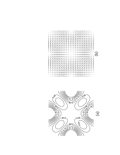
Figure 1.33: Electronic structure of the skyrmion lattice as determined by numerical Hartree-Fock calculations for filling factor $\nu=1.1$ and Zeeman energy $0.015\frac{e^{2}}{\epsilon\ell}$. (a) Excess charge density (in units of $1/(2\pi\ell^{2})$) and (b) Two-dimensional vector representation of the XY components of the spin density. The spin stiffness makes the square lattice more stable than the triangular lattice at this filling factor and Zeeman coupling. Because of the $U(1)$ rotational symmetry about the Zeeman axis, this is simply one representative member of a continuous family of degenerate Hartree-Fock solutions. After Brey et al. [71].

This ‘antiferromagnetic’ arrangement of the XY spin orientation minimizes the spin gradient energy and would be frustrated on the triangular lattice. Hence it is the spin stiffness that stabilizes the square lattice structure.

The Hartree-Fock ground state breaks both global translation and global $U(1)$ spin rotation symmetry. It is a kind of ‘supersolid’ with both diagonal

$$G^{z}\equiv\left\langle s^{z}(\vec{r}\,)\;s^{z}(\vec{r}^{\,\prime})\right\rangle$$ (1.287)

and off-diagonal

$$G^{\perp}\equiv\left\langle s^{+}(\vec{r}\,)\;s^{-}(\vec{r}^{\,\prime})\right\rangle$$ (1.288)

long-range order. For the case of a single skyrmion we found that the $U(1)$ symmetry was broken at the Hartree-Fock (classical) level but fully restored by quantum fluctuations of the zero mode coordinate $\varphi$. In the thermodynamic limit of an infinite number of skyrmions coupled together, it is possible for the global $U(1)$ rotational symmetry breaking to survive quantum fluctuations. If this occurs then an excitation gap is not produced. Instead we have a new kind of gapless spin wave Goldstone mode [74, 75]. This mode is gapless despite the presence of the Zeeman field and hence has a profound effect on the NMR relaxation rate. The gapless Goldstone mode associated with the broken translation symmetry is the ordinary magneto-phonon of the Wigner crystal. This too contributes to the nuclear relaxation rate.

In actual practice, disorder will be important. In addition, the NMR experiments have so far been performed at temperatures which are likely well above the lattice melting temperature. Nevertheless the zero temperature lattice calculations to be discussed below probably capture the essential physics of this non co-linear magnet. Namely, there exist spin fluctuations at frequencies orders of magnitude below the Zeeman gap. At zero temperature these are coherent Goldstone modes. Above the lattice melting temperature they will be overdamped diffusive modes derived from the Goldstone modes. The essential physics will still be that the spin fluctuations have strong spectral density at frequencies far below the Zeeman gap.

It turns out that at long wavelengths the magnetophonon and $U(1)$ spin modes are decoupled. We will therefore ignore the positional degrees of freedom when analyzing the new $U(1)$ mode. We have already found the $U(1)$ Hamiltonian for a single skyrmion in eq. (1.282). The simplest generalization to the Skyrme lattice which is consistent with the symmetries of the problem is

$$H=\frac{U}{2}\sum_{j}(\hat{K}_{j}-K)^{2}-J\sum_{\langle ij\rangle}\cos{(\varphi_{i}-\varphi_{j})}$$ (1.289)

where $\hat{K}_{j}\equiv-i\frac{\partial}{\partial\varphi_{j}}$ is the angular momentum operator. The global $U(1)$ symmetry requires that the interactive term be invariant if all of the $\varphi_{j}$’s are increased by a constant. In addition $H$ must be invariant under $\varphi_{j}\rightarrow\varphi_{j}+2\pi$ for any single skyrmion. We have assumed the simplest possible near-neighbor coupling, neglecting the possibility of longer range higher-order couplings of the form $\cos n(\varphi_{i}-\varphi_{j})$ which are also symmetry allowed. The phenomenological coupling $J$ must be negative to be consistent with the ‘antiferromagnetic’ XY order found in the Hartree-Fock ground state illustrated in fig. (1.33). However we will find it convenient to instead make $J$ positive and compensate for this by a ‘gauge’ change $\varphi_{j}\rightarrow\varphi_{j}+\pi$ on one sublattice. This is convenient because it makes the coupling ‘ferromagnetic’ rather than ‘antiferromagnetic.’

Eq. (1.289) is the Hamiltonian for the quantum XY rotor model, closely related to the boson Hubbard model [76, 77, 78]. Readers familiar with superconductivity will recognize that this model is commonly used to describe the superconductor-insulator transition in Josephson arrays [76, 77]. The angular momentum eigenvalue of the $\hat{K}_{j}$ operator represents the number of bosons (Cooper pairs) on site $j$ and the $U$ term describes the charging energy cost when this number deviates from the electrostatically optimal value of $K$. The boson number is non-negative while $\hat{K}_{j}$ has negative eigenvalues. However we assume that $K\gg 1$ so that the negative angular momentum states are very high in energy.

The $J$ term in the quantum rotor model is a mutual torque that transfers units of angular momentum between neighboring sites. In the boson language the wave function for the state with $m$ bosons on site $j$ contains a factor

$$\psi_{m}(\varphi_{j})=e^{im\varphi_{j}}.$$ (1.290)

The raising and lowering operators are thus $e^{\pm i\varphi_{j}}$. This shows us that the cosine term in eq. (1.289) represents the Josephson coupling that hops bosons between neighboring sites.

For $U\gg J$ the system is in an insulating phase well-described by the wave function

$$\psi(\varphi_{1},\varphi_{2},\ldots,\varphi_{N})=\prod_{j}e^{im\varphi_{j}}$$ (1.291)

where $m$ is the nearest integer to $K$. In this state every rotor has the same fixed angular momentum and thus every site has the same fixed particle number in the boson language. There is a large excitation gap

$$\Delta\approx U\left(1-2|m-K|\right)$$ (1.292)

and the system is insulating.

Clearly $|\psi|^{2}\approx 1$ in this phase and it is therefore quantum disordered. That is, the phases $\{\varphi_{j}\}$ are wildly fluctuating because every configuration is equally likely. The phase fluctuations are nearly uncorrelated

$$\langle e^{i\varphi_{j}}\;e^{-i\varphi_{k}}\rangle\sim e^{-|\vec{r}_{j}-\vec{r}_{k}|/\xi}.$$ (1.293)

For $J\gg U$ the phases on neighboring sites are strongly coupled together and the system is a superconductor. A crude variational wave function that captures the essential physics is

$$\psi(\varphi_{1},\varphi_{2},\ldots,\varphi_{N})\sim e^{\lambda\sum_{\langle ij\rangle}\;\cos{(\varphi_{i}-\varphi_{j})}}$$ (1.294)

where $\lambda$ is a variational parameter [79]. This is the simplest ansatz consistent with invariance under $\varphi_{j}\rightarrow\varphi_{j}+2\pi$. For $J\gg U$, $\lambda\gg 1$ and $|\psi|^{2}$ is large only for spin configurations with all of the XY spins locally parallel. Expanding the cosine term in eq. (1.289) to second order gives a harmonic Hamiltonian which can be exactly solved. The resulting gapless ‘spin waves’ are the Goldstone modes of the superconducting phase.

For simplicity we work with the Lagrangian rather than the Hamiltonian

$$\mathcal{L}=\sum_{j}\left[\hbar K\dot{\varphi}_{j}+\frac{\hbar^{2}}{2U}\dot{\varphi}_{j}^{2}\right]+J\sum_{\langle ij\rangle}\cos{(\varphi_{i}-\varphi_{j})}$$ (1.295)

The Berry phase term is a total derivative and can not affect the equations of motion. Dropping this term and expanding the cosine in the harmonic approximation yields

$$\mathcal{L}=\frac{\hbar^{2}}{2U}\sum_{j}\dot{\varphi}_{j}^{2}-\frac{J}{2}\sum_{\langle ij\rangle}(\varphi_{i}-\varphi_{j})^{2}.$$ (1.296)

This ‘phonon’ model has linearly dispersing gapless collective modes at small wavevectors

$$\hbar\omega_{q}=\sqrt{UJ}\;qa$$ (1.297)

where $a$ is the lattice constant. The parameters $U$ and $J$ can be fixed by fitting to microscopic Hartree-Fock calculations of the spin wave velocity and the magnetic susceptibility (‘boson compressibility’) [61, 75]. This in turn allows one to estimate the regime of filling factor and Zeeman energy in which the $U(1)$ symmetry is not destroyed by quantum fluctuations [75].

Let us now translate all of this into the language of our non-colinear QHE ferromagnet [74, 75]. Recall that the angular momentum (the ‘charge’) conjugate to the phase angle $\varphi$ is the spin angular momentum of the overturned spins that form the skyrmion. In the quantum disordered ‘insulating’ phase, each skyrmion has a well defined integer-valued ‘charge’ (number of overturned spins) much like we found when we quantized the $U(1)$ zero mode for the plane angle $\varphi$ of a single isolated skyrmion in eq. (1.283). There is an excitation gap separating the energies of the discrete quantized values of the spin.

The ‘superfluid’ state with broken $U(1)$ symmetry is a totally new kind of spin state unique to non-colinear magnets [74, 75]. Here the phase angle is well-defined and the number of overturned spins is uncertain. The off-diagonal long-range order of a superfluid becomes

$$\langle b_{j}^{\dagger}b_{k}^{\phantom{\dagger}}\rangle\rightarrow\langle e^{i\varphi_{j}}e^{-i\varphi_{k}}\rangle$$ (1.298)

or in the spin language

$$\left\langle s^{+}(\vec{r}\,)s^{-}(\vec{r}^{\,\prime})\right\rangle.$$ (1.299)

Thus in a sense we can interpret a spin flip interaction between an electron and a nucleus as creating a boson in the superfluid. But this boson has a finite probability of ‘disappearing’ into the superfluid ‘condensate’ and hence the system does not have to pay the Zeeman price to create the flipped spin. That is, the superfluid state has an uncertain number of flipped spins (even though $S_{\mathrm{tot}}^{z}$ commutes with $H$) and so the Zeeman energy cost is uncertain.

In classical language the skyrmions locally have finite (slowly varying) x and y spin components which act as effective magnetic fields around which the nuclear spins precess and which thus cause $I^{z}$ to change with time. The key here is that $s^{x}$ and $s^{y}$ can, because of the broken $U(1)$ symmetry, fluctuate very slowly (i.e. at MHz frequencies that the nuclei can follow rather than just the very high Zeeman precession frequency).

Detailed numerical calculations [75] show that the Skyrme lattice is very efficient at relaxing the nuclei and $1/T_{1}$ and is enhanced by a factor of $\sim 10^{3}$ over the corresponding rate at zero magnetic field. We expect this qualitative distinction to survive even above the Skryme lattice melting temperature for the reasons discussed earlier.

Because the nuclear relaxation rate increases by orders of magnitude, the equilibration time at low temperatures drops from hours to seconds. This means that the nuclei come into thermal equilibrium with the electrons and hence the lattice. The nuclei therefore have a well-defined temperature and contribute to the specific heat. Because the temperature is much greater than the nuclear Zeeman energy scale $\Delta\sim 1~{}\mbox{mK}$, each nucleus contributes only a tiny amount $\sim k_{\mathrm{B}}\frac{\Delta^{2}}{T^{2}}$ to the specific heat. On the other hand, the electronic specific heat per particle $\sim k_{\mathrm{B}}\frac{T}{T_{\mathrm{fermi}}}$ is low and the electron density is low. In fact there are about $10^{6}$ nuclei per quantum well electron and the nuclei actually enhance the specific heat more than 5 orders of magnitude [67]!

Surprisingly, at around 30 mK there is a further enhancement of the specific heat by an additional order of magnitude. This may be a signal of the Skyrme lattice melting transition [67, 75, 80], although the situation is somewhat murky at the present time. The peak can not possibly be due to the tiny amount of entropy change in the Skyrme lattice itself. Rather it is due to the nuclei in the thick AlAs barrier between the quantum wells.

1.12 Double-Layer Quantum Hall Ferromagnets

1.12.1 Introduction

We learned in our study of quantum Hall ferromagnets that the Coulomb interaction plays an important role at Landau level filling factor $\nu=1$ because it causes the electron spins to spontaneously align ferromagnetically and this in turn profoundly alters the charge excitation spectrum by producing a gap. A closely related effect occurs in double-layer systems in which layer index is analogous to spin [81, 44, 43]. Building on our knowledge of the dynamics of ferromagnets developed in the last section, we will use this analogy to explore the rich physics of double-layer systems.

Novel fractional quantum Hall effects due to correlations [82] in multicomponent systems were anticipated in early work by Halperin [42] and the now extensive literature has been reviewed in [43]. There have also been recent interesting studies of systems in which the spin and layer degrees of freedom are coupled in novel ways [83, 84].

As described in this volume by Shayegan [45], modern MBE techniques make it possible to produce double-layer (and multi-layer) two-dimensional electron gas systems of extremely low disorder and high mobility. As illustrated schematically in Fig. (1.34),

Figure 1.34: Schematic conduction band edge profile for a double-layer two-dimensional electron gas system. Typical widths and separations are $W\sim d\sim 100\hbox{\AA}$ and are comparable to the spacing between electrons within each inversion layer.

these systems consist of a pair of 2D electron gases separated by a distance $d$ so small ($d\sim 100\mbox{\AA}$) as to be comparable to the typical spacing between electrons in the same layer. A second type of system has also recently been developed to a high degree of perfection [85]. These systems consist of single wide quantum wells in which strong mixing of the two lowest electric subbands allows the electrons to localize themselves on opposites sides of the well to reduce their correlation energy. We will take the point of view that these systems can also be approximately viewed as double-well systems with some effective layer separation and tunnel barrier height.

As we have already learned, correlations are especially important in the strong magnetic field regime because all electrons can be accommodated within the lowest Landau level and execute cyclotron orbits with a common kinetic energy. The fractional quantum Hall effect occurs when the system has a gap for making charged excitations, i.e. when the system is incompressible. Theory has predicted [42, 82, 86] that at some Landau level filling factors, gaps occur in double-layer systems only if interlayer interactions are sufficiently strong. These theoretical predictions have been confirmed [87]. More recently work from several different points of view [88, 89, 90, 91, 92, 93] has suggested that inter-layer correlations can also lead to unusual broken symmetry states with a novel kind of spontaneous phase coherence between layers which are isolated from each other except for inter-layer Coulomb interactions. It is this spontaneous interlayer phase coherence which is responsible [73, 51, 94, 43] for a variety of novel features seen in the experimental data to be discussed below [81, 44].

1.12.2 Pseudospin Analogy

We will make the simplifying assumption that the Zeeman energy is large enough that fluctuations of the (true) spin order can be ignored, leaving out the possibility of mixed spin and pseudospin correlations [83, 84]. We will limit our attention to the lowest electric subband of each quantum well (or equivalently, the two lowest bands of a single wide well). Hence we have a two-state system that can be labeled by a pseudospin 1/2 degree of freedom. Pseudospin up means that the electron is in the (lowest electric subband of the) upper layer and pseudospin down means that the electron is in the (lowest electric subband of the) lower layer.

Just as in our study of ferromagnetism we will consider states with total filling factor $\nu\equiv\nu_{\uparrow}+\nu_{\downarrow}=1$. A state exhibiting interlayer phase coherence and having the pseudospins ferromagnetically aligned in the direction defined by polar angle $\theta$ and azimuthal angle $\varphi$ can be written in the Landau gauge just as for ordinary spin

$$|\psi\rangle=\prod_{k}\left\{\cos(\theta/2)c^{\dagger}_{k\uparrow}+\sin(\theta/2)e^{i\varphi}c^{\dagger}_{k\downarrow}\right\}|0\rangle.$$ (1.300)

Every $k$ state contains one electron and hence this state has $\nu=1$ as desired. Note however that the layer index for each electron is uncertain. The amplitude to find a particular electron in the upper layer is $\cos(\theta/2)$ and the amplitude to find it in the lower layer is $\sin(\theta/2)e^{i\varphi}$. Even if the two layers are completely independent with no tunneling between them, quantum mechanics allows for the somewhat peculiar possibility that we are uncertain which layer the electron is in.

For the case of ordinary spin we found that the Coulomb interaction produced an exchange energy which strongly favored having the spins locally parallel. Using the fact that the Coulomb interaction is completely spin independent (it is only the Pauli principle that indirectly induces the ferromagnetism) we wrote down the spin rotation invariant effective theory in eq. (1.231). Here we do not have full SU(2) invariance because the interaction between electrons in the same layer is clearly stronger than the interaction between electrons in opposite layers. Thus for example, if all the electrons are in the upper (or lower) layer, the system will look like a charged capacitor and have higher energy than if the layer occupancies are equal. Hence to leading order in gradients we expect the effective action to be modified slightly

$$\mathcal{L}= - \int d^{2}r\;\left\{\hbar Sn\,\dot{m}^{\mu}(\vec{r}\,)\mathcal{A}^{\mu}[\vec{m}]-\lambda(\vec{r}\,)(m^{\mu}m^{\mu}-1)\right\}$$ (1.301)

$$- \int d^{2}r\,\left\{\frac{1}{2}\rho_{s}\partial_{\mu}m^{\nu}\partial_{\mu}m^{\nu}+\beta m^{z}m^{z}-\Delta m^{z}-ntm^{x}\right\}.$$

The spin stiffness $\rho_{s}$ represents the SU(2) invariant part of the exchange energy and is therefore somewhat smaller than the value computed in eq. (1.238). The coefficient $\beta$ is a measure of the capacitive charging energy. The analog of the Zeeman energy $\Delta$ represents an external electric field applied along the MBE growth direction which unbalances the charge densities in the two layers. The coefficient $t$ represents the amplitude for the electrons to tunnel between the two layers. It prefers the pseudospin to be aligned in the $\hat{x}$ direction because this corresponds to the spinor

$$\frac{1}{\sqrt{2}}\left(\begin{array}[]{c}1\\ 1\end{array}\right)$$ (1.302)

which represents the symmetric (i.e. bonding) linear combination of the two well states. The state with the pseudospin pointing in the $-\hat{x}$ direction represents the antisymmetric (i.e. antibonding) linear combination which is higher in energy.

For the moment we will assume that both $t$ and $\Delta$ vanish, leaving only the $\beta$ term which breaks the pseudospin rotational symmetry. The case $\beta<0$ would represent ‘Ising anisotropy’. Clearly the physically realistic case for the capacitive energy gives $\beta>0$ which represents so-called ‘easy plane anisotropy.’ The energy is minimized when $m^{z}=0$ so that the order parameter lies in the XY plane giving equal charge densities in the two layers. Thus we are left with an effective XY model which should exhibit long-range off-diagonal order

$$\Psi(\vec{r}\,)=\langle m^{x}(\vec{r}\,)+im^{y}(\vec{r}\,)\rangle.$$ (1.303)

The order is ‘off-diagonal’ because it corresponds microscopically to an operator

$$\Psi(\vec{r}\,)=\langle s^{+}(\vec{r}\,)\rangle=\langle\psi^{\dagger}_{\uparrow}(\vec{r}\,)\psi_{\downarrow}(\vec{r}\,)\rangle$$ (1.304)

which is not diagonal in the $s^{z}$ basis, much as in a superfluid where the field operator changes the particle number and yet it condenses and acquires a finite expectation value.

One other comment worth making at this point is that eq. (1.304) shows that, unlike the order parameter in a superconductor or superfluid, this one corresponds to a charge neutral operator. Hence it will be able to condense despite the strong magnetic field (which fills charged condensates with vortices and generally destroys the order).

In the next subsection we review the experimental evidence that long-range XY correlations exist and that as a result, the system exhibits excitations which are highly collective in nature. After that we will return to further analysis and interpretation of the effective Lagrangian in eq. (1.301) to understand those excitations.

1.12.3 Experimental Background

As illustrated by the dashed lines in fig. (1.34), the lowest energy eigenstates split into symmetric and antisymmetric combinations separated by an energy gap $\Delta_{\mathrm{SAS}}=2t$ which can, depending on the sample, vary from essentially zero to many hundreds of Kelvins. The splitting can therefore be much less than or greater than the interlayer interaction energy scale, $E_{\mathrm{c}}\equiv e^{2}/\epsilon d$. Thus it is possible to make systems which are in either the weak or strong correlation limits.

When the layers are widely separated, there will be no correlations between them and we expect no dissipationless quantum Hall state since each layer has [95] $\nu=1/2$. For smaller separations, it is observed experimentally that there is an excitation gap and a quantized Hall plateau [96, 85, 81]. This has either a trivial or a highly non-trivial explanation, depending on the ratio $\Delta_{\mathrm{SAS}}/E_{\mathrm{c}}$. For large $\Delta_{\mathrm{SAS}}$ the electrons tunnel back and forth so rapidly that it is as if there is only a single quantum well. The tunnel splitting $\Delta_{\mathrm{SAS}}$ is then analogous to the electric subband splitting in a (wide) single well. All symmetric states are occupied and all antisymmetric states are empty and we simply have the ordinary $\nu=1$ integer Hall effect. Correlations are irrelevant in this limit and the excitation gap is close to the single-particle gap $\Delta_{\mathrm{SAS}}$ (or $\hbar\omega_{\mathrm{c}}$, whichever is smaller). What is highly non-trivial about this system is the fact that the $\nu=1$ quantum Hall plateau survives even when $\Delta_{\mathrm{SAS}}\ll E_{\mathrm{c}}$. In this limit the excitation gap has clearly changed to become highly collective in nature since the observed [85, 81] gap can be on the scale of 20K even when $\Delta_{\mathrm{SAS}}\sim 1~{}\mathrm{K}$. Because of the spontaneously broken XY symmetry [88, 89, 92, 73, 51], the excitation gap actually survives the limit $\Delta_{\mathrm{SAS}}\longrightarrow 0$! This cross-over from single-particle to collective gap is quite analogous to that for spin polarized single layers. There the excitation gap survives the limit of zero Zeeman splitting so long as the Coulomb interaction makes the spin stiffness non-zero. This effect in double-layer systems is visible in fig. (1.35)

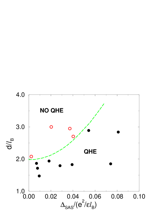
Figure 1.35: Phase diagram for the double layer QHE system (after Murphy et al. [81]). Only samples whose parameters lie below the dashed line exhibit a quantized Hall plateau and excitation gap.

which shows the QHE phase diagram obtained by Murphy et al.[81, 44] as a function of layer-separation and tunneling energy. A $\nu=1$ quantum Hall plateau and gap is observed in the regime below the dashed line. Notice that far to the right, the single particle tunneling energy dominates over the coulomb energy and we have essentially a one-body integer QHE state. However the QHE survives all the way into $\Delta_{\mathrm{SAS}}=0$ provided that the layer separation is below a critical value $d/\ell_{\mathrm{B}}\approx 2$. In this limit there is no tunneling and the gap is purely many-body in origin and, as we will show, is associated with the remarkable ‘pseudospin ferromagnetic’ quantum state exhibiting spontaneous interlayer phase coherence.

A second indication of the highly collective nature of the excitations can be seen in the Arrhenius plots of thermally activated dissipation [81] shown in the inset of fig. (1.36)

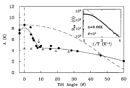
Figure 1.36: The charge activation energy gap, $\Delta$, as a function of tilt angle in a weakly tunneling double-layer sample ($\Delta_{\mathrm{SAS}}=0.8$K). The solid circles are for filling $\nu=1$, open triangles for $\nu=2/3$. The arrow indicates the critical angle $\theta_{\mathrm{c}}$. The solid line is a guide to the eye. The dashed line refers to a simple estimate of the renormalization of the tunneling amplitude by the parallel magnetic field. Relative to the actual decrease, this one-body effect is very weak and we have neglected it. Inset: Arrhenius plot of dissipation. The low temperature activation energy is $\Delta=8.66$K and yet the gap collapses at a much lower temperature scale of about $0.4$K ($1/T\approx 2.5$). (After Murphy et al. [81]).

The low temperature activation energy $\Delta$ is, as already noted, much larger than $\Delta_{\mathrm{SAS}}$. If $\Delta$ were nevertheless somehow a single-particle gap, one would expect the Arrhenius law to be valid up to temperatures of order $\Delta$. Instead one observes a fairly sharp leveling off in the dissipation as the temperature increases past values as low as $\sim 0.05\Delta$. This is consistent with the notion of a thermally induced collapse of the order that had been producing the collective gap.

The third significant feature of the experimental data pointing to a highly-ordered collective state is the strong response of the system to relatively weak magnetic fields $B_{\parallel}$ applied in the plane of the 2D electron gases. In fig. (1.36) we see that the charge activation gap drops dramatically as the magnetic field is tilted (keeping $B_{\perp}$ constant).

Within a model that neglects higher electric subbands, we can treat the electron gases as strictly two-dimensional. This is important since $B_{\parallel}$ can affect the system only if there are processes that carry electrons around closed loops containing flux. A prototypical such process is illustrated in fig. (1.37).

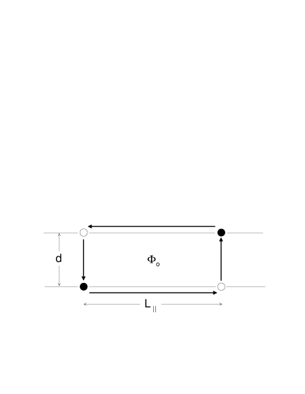
Figure 1.37: A process in a double-layer two-dimensional electron gas system which encloses flux from the parallel component of the magnetic field. One interpretation of this process is that an electron tunnels from the upper layer to the lower layer (near the left end of the figure). The resulting particle-hole pair then travels coherently to the right and is annihilated by a subsequent tunneling event in the reverse direction. The quantum amplitude for such paths is sensitive to the parallel component of the field.

An electron tunnels from one layer to the other at point A, and travels to point B. Then it (or another indistinguishable electron) tunnels back and returns to the starting point. The parallel field contributes to the quantum amplitude for this process (in the 2D gas limit) a gauge-invariant Aharonov-Bohm phase factor $\exp\left(2\pi i\Phi/\Phi_{0}\right)$ where $\Phi$ is the enclosed flux and $\Phi_{0}$ is the quantum of flux.

Such loop paths evidently contribute significantly to correlations in the system since the activation energy gap is observed to decrease very rapidly with $B_{\parallel}$, falling by factors of order two or more until a critical field, $B^{*}_{\parallel}\sim 0.8\mathrm{T}$, is reached at which the gap essentially ceases changing [81]. To understand how remarkably small $B^{*}_{\parallel}$ is, consider the following. We can define a length $L_{\parallel}$ from the size of the loop needed to enclose one quantum of flux: $L_{\parallel}B^{*}_{\parallel}d=\Phi_{0}$. ($L_{\parallel}[\hbox{\AA}]=4.137\times 10^{5}/d[\hbox{\AA}]B^{*}_{\parallel}[\mathrm{T}]$.) For $B^{*}_{\parallel}=0.8\mathrm{T}$ and $d=150\hbox{\AA}$, $L_{\parallel}=2700\hbox{\AA}$ which is approximately twenty times the spacing between electrons in a given layer and thirty times larger than the quantized cyclotron orbit radius $\ell\equiv(\hbar c/eB_{\perp})^{1/2}$ within an individual layer. Significant drops in the excitation gap are already seen at fields of 0.1T implying enormous phase coherent correlation lengths must exist. Again this shows the highly-collective long-range nature of the ordering in this system.

In the next subsection we shall briefly outline a detailed model which explains all these observed effects.

1.12.4 Interlayer Phase Coherence

The essential physics of spontaneous inter-layer phase coherence can be examined from a microscopic point of view [90, 91, 92, 73, 51] or a macroscopic Chern-Simons field theory point of view [88, 89, 73, 51], but it is perhaps most easily visualized in the simple variational wave function which places the spins purely in the XY plane [51]

$$|\psi\rangle=\prod_{k}\left\{c^{\dagger}_{k\uparrow}+c^{\dagger}_{k\downarrow}e^{i\varphi}\right\}|0\rangle.$$ (1.305)

Note for example, that if $\varphi=0$ then we have precisely the non-interacting single Slater determinant ground state in which electrons are in the symmetric state which, as discussed previously in the analysis of the effective Lagrangian in eq. (1.301), minimizes the tunneling energy. This means that the system has a definite total number of particles ($\nu=1$ exactly) but an indefinite number of particles in each layer. In the absence of inter-layer tunneling, the particle number in each layer is a good quantum number. Hence this wave function represents a state of spontaneously broken symmetry [88, 89, 51] in the same sense that the BCS state for a superconductor has indefinite (total) particle number but a definite phase relationship between states of different particle number.

In the absence of tunneling ($t=0$) the energy can not depend on the phase angle $\varphi$ and the system exhibits a global $U(1)$ symmetry associated with conservation of particle number in each layer [88]. One can imagine allowing $\varphi$ to vary slowly with position to produce excited states. Given the $U(1)$ symmetry, the effective Hartree-Fock energy functional for these states is restricted to have the leading form

$$H=\frac{1}{2}\rho_{s}\int d^{2}r|\nabla\varphi|^{2}+\ldots\,\,.$$ (1.306)

The origin of the finite ‘spin stiffness’ $\rho_{s}$ is the loss of exchange energy which occurs when $\varphi$ varies with position. Imagine that two particles approach each other. They are in a linear superposition of states in each of the layers (even though there is no tunneling!). If they are characterized by the same phase $\varphi$, then the wave function is symmetric under pseudospin exchange and so the spatial wave function is antisymmetric and must vanish as the particles approach each other. This lowers the Coulomb energy. If a phase gradient exists then there is a larger amplitude for the particles to be near each other and hence the energy is higher. This loss of exchange energy is the source of the finite spin stiffness and is what causes the system to spontaneously ‘magnetize’.

We see immediately that the $U(1)$ symmetry leads to eq. (1.306) which defines an effective XY model which will contain vortex excitations which interact logarithmically. [97, 98] In a superconducting film the vortices interact logarithmically because of the kinetic energy cost of the supercurrents circulating around the vortex centers. Here the same logarithm appears, but it is due to the potential energy cost (loss of exchange) associated with the phase gradients (circulating pseudo-spin currents).

Hartree-Fock estimates [51] indicate that the spin stiffness $\rho_{s}$ and hence the Kosterlitz-Thouless (KT) critical temperature are on the scale of 0.5 K in typical samples. Vortices in the $\varphi$ field are reminiscent of Laughlin’s fractionally charged quasiparticles but in this case carry charges $\pm\frac{1}{2}e$ and can be left- or right-handed for a total of four ‘flavors’ [73, 51]. It is also possible to show [51, 94] that the presence of spontaneous magnetization due to the finite spin stiffness means that the charge excitation gap is finite (even though the tunnel splitting is zero). Thus the QHE survives [51] the limit $\Delta_{\mathrm{SAS}}\longrightarrow 0$.

Since the ‘charge’ conjugate to the phase $\varphi$ is the $z$ component of the pseudo spin $S^{z}$, the pseudospin ‘supercurrent’

$$\vec{J}=\rho_{s}\mathbf{\vec{\nabla}}\varphi$$ (1.307)

represents oppositely directed charge currents in each layer. Below the KT transition temperature, such current flow will be dissipationless (in linear response) just as in an ordinary superfluid. Likewise there will be a linearly dispersing collective Goldstone mode as in a superfluid [90, 88, 89, 73, 51] rather than a mode with quadratic dispersion as in the SU(2) symmetric ferromagnet. (This is somewhat akin to the difference between an ideal bose gas and a repulsively interacting bose gas.)

If found, this Kosterlitz-Thouless transition would be the first example of a finite-temperature phase transition in a QHE system. The transition itself has not yet been observed due to the tunneling amplitude $t$ being significant in samples having the layers close enough together to have strong correlations. As we have seen above however, significant effects which imply the existence of long-range XY order correlations have been found. Whether or not an appropriate sample can be constructed to observe the phase transition is an open question at this point.

Exercise 1.23

Following the method used to derive eq. (1.237), show that the collective mode for the Lagrangian in eq. (1.301) has linear rather than quadratic dispersion due to the presence of the $\beta$ term. (Assume $\Delta=t=0$.) Hint: Consider small fluctuations of the magnetization away from $\vec{m}=(1,0,0)$ and choose an appropriate gauge for $\cal A$ for this circumstance. Present a qualitative argument that layer imbalance caused by $\Delta$ does not fundamentally change any of the results described in this section but rather simply renormalizes quantities like the collective mode velocity. That is, explain why the $\nu=1$ QHE state is robust against charge imbalance. (This is an important signature of the underlying physics. Certain other interlayer correlated states (such as the one at total filling $\nu=1/2$) are quite sensitive to charge imbalance [43].)

1.12.5 Interlayer Tunneling and Tilted Field Effects

As mentioned earlier, a finite tunneling amplitude $t$ between the layers breaks the $U(1)$ symmetry

$$H_{\mathrm{eff}}=\int d^{2}r\left[\frac{1}{2}\rho_{s}|\nabla\varphi|^{2}-nt\cos{\varphi}\right]$$ (1.308)

by giving a preference to symmetric tunneling states. This can be seen from the tunneling Hamiltonian

$$H_{\mathrm{T}}=-t\int d^{2}r\left\{\psi_{\uparrow}^{\dagger}(\mathbf{r})\psi_{\downarrow}(\mathbf{r})+\psi_{\downarrow}^{\dagger}(\mathbf{r})\psi_{\uparrow}(\mathbf{r})\right\}$$ (1.309)

which can be written in the spin representation as

$$H_{\mathrm{T}}=-2t\int d^{2}rS^{x}(\mathbf{r}).$$ (1.310)

(Recall that the eigenstates of $S^{x}$ are symmetric and antisymmetric combinations of up and down.)

As the separation $d$ increases, a critical point $d^{*}$ is reached at which the magnetization vanishes and the ordered phase is destroyed by quantum fluctuations [73, 51]. This is illustrated in fig. (1.35). For finite tunneling $t$, we will see below that the collective mode becomes massive and quantum fluctuations will be less severe. Hence the phase boundary in fig. (1.35) curves upward with increasing $\Delta_{\mathrm{SAS}}$.

The introduction of finite tunneling amplitude destroys the U(1) symmetry and makes the simple vortex-pair configuration extremely expensive. To lower the energy the system distorts the spin deviations into a domain wall or ‘string’ connecting the vortex cores as shown in fig. (1.38).

Figure 1.38: Meron pair connected by a domain wall. Each meron carries a charge $e/2$ which tries to repel the other one.

The spins are oriented in the $\hat{x}$ direction everywhere except in the central domain wall region where they tumble rapidly through $2\pi$. The domain wall has a fixed energy per unit length and so the vortices are now confined by a linear ‘string tension’ rather than logarithmically. We can estimate the string tension by examining the energy of a domain wall of infinite length. The optimal form for a domain wall lying along the $y$ axis is given by

$$\varphi(\vec{r})=2\arcsin{[\tanh{(\lambda x)}]},$$ (1.311)

where the characteristic width of the string is

$$\lambda^{-1}=\left[\frac{2\pi\ell^{2}\rho_{s}}{t}\right]^{\frac{1}{2}}.$$ (1.312)

The resulting string tension is

$$T_{0}=8\left[\frac{t\rho_{s}}{2\pi\ell^{2}}\right]^{\frac{1}{2}}.$$ (1.313)

Provided the string is long enough ($R\lambda\gg 1$), the total energy of a segment of length $R$ will be well-approximated by the expression

$$E_{\mathrm{pair}}^{\prime}=2E_{\mathrm{mc}}^{\prime}+\frac{e^{2}}{4R}+T_{0}R.$$ (1.314)

This is minimized at $R^{*}=\sqrt{e^{2}/4T_{0}}$. The linear confinement brings the charged vortices closer together and rapidly increases the Coulomb energy. In the limit of very large tunneling, the meron pair shrinks and the single-particle excitation (hole or extra spin-reversed electron) limit must be recovered.

The presence of parallel field $B_{\parallel}$ field can be conveniently described with the gauge choice

$$\vec{A}_{\parallel}=xB_{\parallel}\hat{z}$$ (1.315)

where $\hat{z}$ is the growth direction. In this gauge the tunneling amplitude transforms to

$$t\rightarrow t\;e^{iQx}$$ (1.316)

and the energy becomes

$$H=\int d^{2}r\left[\frac{1}{2}\rho_{s}|\vec{\nabla}\varphi|^{2}-\frac{t}{2\pi\ell^{2}}\cos{(\varphi-Qx)}\right]$$ (1.317)

where $Q=2\pi/L_{\parallel}$ and $L_{\parallel}$ is the length associated with one quantum of flux for the loops shown in fig. 1.37. This is the so-called Pokrovsky-Talopov model which exhibits a commensurate-incommensurate phase transition. At low $B_{\parallel}$, $Q$ is small and the low energy state has $\varphi\approx Qx$; i.e. the local spin orientation ‘tumbles’. In contrast, at large $B_{\parallel}$ the gradient cost is too large and we have $\varphi\approx\hbox{constant}$. It is possible to show [51, 94] that this phase transition semiquantitatively explains the rapid drop and subsequent leveling off of the activation energy vs. $B_{\parallel}$ seen in fig. (1.36).

Exercise 1.24

Derive eq. (1.311) for the form of the ‘soliton’ that minimizes the energy cost for the Hamiltonian in eq. (1.308).

1.13 Acknowledgments

Much of my work on the quantum Hall effect has been in collaboration with Allan MacDonald. The more recent work on quantum Hall ferromagnets has also been done in collaboration with M. Abolfath, L. Belkhir, L. Brey, R. Côté, H. Fertig, P. Henelius, K. Moon, H. Mori, J. J. Palacios, A. Sandvik, H. Stoof, C. Timm, K. Yang, D. Yoshioka, S. C. Zhang, and L. Zheng. It is a pleasure to acknowledge many useful conversations with S. Das Sarma, M. P. A. Fisher, N. Read, and S. Sachdev.

It is a pleasure to thank Ms. Daphne Klemme for her expert typesetting of my scribbled notes and Jairo Sinova for numerous helpful comments on the manuscript.

This work was supported by NSF DMR-9714055.

Appendix A Lowest Landau Level Projection

A convenient formulation of quantum mechanics within the subspace of the lowest Landau level (LLL) was developed by Girvin and Jach [26], and was exploited by Girvin, MacDonald and Platzman in the magneto-roton theory of collective excitations of the incompressible states responsible for the fractional quantum Hall effect [29]. Here we briefly review this formalism. See also Ref. [8].

We first consider the one-body case and choose the symmetric gauge. The single-particle eigenfunctions of kinetic energy and angular momentum in the LLL are given in Eq. (1.76)

$$\phi_{m}(z)=\frac{1}{(2\pi 2^{m}m!)^{1/2}}\>z^{m}\>\exp{\biggl{(}-\frac{|z|^{2}}{4}\biggr{)}},$$ (A.1)

where $m$ is a non-negative integer, and $z=(x+iy)/\ell$. From (A.1) it is clear that any wave function in the LLL can be written in the form

$$\psi(z)=f(z)\>e^{-\frac{|z|^{2}}{4}}$$ (A.2)

where $f(z)$ is an analytic function of $z$, so the subspace in the LLL is isomorphic to the Hilbert space of analytic functions [26, 99, 8]. Following Bargman [26, 99], we define the inner product of two analytic functions as

$$(f,g)=\int d\mu(z)\>f^{\ast}(z)\>g(z),$$ (A.3)

where

$$d\mu(z)\equiv(2\pi)^{-1}\>dxdy\>e^{-\frac{|z|^{2}}{2}}.$$ (A.4)

Now we can define bosonic ladder operators that connect $\phi_{m}$ to $\phi_{m\pm 1}$ (and which act on the polynomial part of $\phi_{m}$ only):

$$a^{\dagger} = {z\over\sqrt{2}},$$ (A.5a)

$$a = \sqrt{2}\>\frac{\partial}{\partial z},$$ (A.5b)

so that

$$a^{\dagger}\>\varphi_{m} = \sqrt{m+1}\>\varphi_{m+1},$$ (A.6a)

$$a\>\varphi_{m} = \sqrt{m}\>\varphi_{m-1},$$ (A.6b)

$$(f,a^{\dagger}\;g) = (a\;f,g),$$ (A.6c)

$$(f,a\;g) = (a^{\dagger}\;f,g).$$ (A.6d)

All operators that have non-zero matrix elements only within the LLL can be expressed in terms of $a$ and $a^{\dagger}$. It is essential to notice that the adjoint of $a^{\dagger}$ is not $z^{\ast}/\sqrt{2}$ but $a\equiv\sqrt{2}\partial/\partial z$, because $z^{\ast}$ connects states in the LLL to higher Landau levels. Actually $a$ is the projection of $z^{\ast}/\sqrt{2}$ onto the LLL as seen clearly in the following expression:

$$(f,\frac{z^{\ast}}{\sqrt{2}}\;g)=(\frac{z}{\sqrt{2}}\;f,g)=(a^{\dagger}\;f,g)=(f,a\;g).$$

So we find

$$\overline{z^{\ast}}=2\frac{\partial}{\partial z},$$ (A.7)

where the overbar indicates projection onto the LLL. Since $\overline{z^{\ast}}$ and $z$ do not commute, we need to be very careful to properly order the operators before projection. A little thought shows that in order to project an operator which is a combination of $z^{\ast}$ and $z$, we must first normal order all the $z^{\ast}$’s to the left of the $z$’s, and then replace $z^{\ast}$ by $\overline{z^{\ast}}$. With this rule in mind and (A.7), we can easily project onto the LLL any operator that involves space coordinates only.

For example, the one-body density operator in momentum space is

$$\rho_{\mathbf{q}}=\frac{1}{\sqrt{A}}\>e^{-i\mathbf{q}\cdot\mathbf{r}}=\frac{1}{\sqrt{A}}\>e^{-\frac{i}{2}(q^{\ast}z+qz^{\ast})}=\frac{1}{\sqrt{A}}\>e^{-\frac{i}{2}qz^{\ast}}\;e^{-\frac{i}{2}q^{\ast}z},$$

where $A$ is the area of the system, and $q=q_{x}+iq_{y}$. Hence

$$\overline{\rho_{q}}=\frac{1}{\sqrt{A}}\>e^{-iq\frac{\partial}{\partial z}}\;e^{-\frac{i}{2}q^{\ast}z}=\frac{1}{\sqrt{A}}\>e^{-\frac{|q|^{2}}{4}}\;\tau_{q},$$ (A.8)

where

$$\tau_{q}=e^{-iq\frac{\partial}{\partial z}-\frac{i}{2}q^{\ast}z}$$ (A.9)

is a unitary operator satisfying the closed Lie algebra

$$\tau_{q}\tau_{k} = \tau_{q+k}\>e^{\frac{i}{2}q\wedge k},$$ (A.10a)

$${}[\tau_{q},\tau_{k}] = 2i\;\tau_{q+k}\>\sin{\frac{q\wedge k}{2}},$$ (A.10b)

where $q\wedge k\equiv\ell^{2}(\mathbf{q}\times\mathbf{k})\cdot\hat{\mathbf{z}}$. We also have $\tau_{q}\tau_{k}\>\tau_{-q}\tau_{-k}=e^{iq\wedge k}$. This is a familiar feature of the group of translations in a magnetic field, because $q\wedge k$ is exactly the phase generated by the flux in the parallelogram generated by $\mathbf{q}\ell^{2}$ and $\mathbf{k}\ell^{2}$. Hence the $\tau$’s form a representation of the magnetic translation group [see Fig. (A.1)].

Figure A.1: Illustration of magnetic translations and phase factors. When an electron travels around a parallelogram (generated by $\tau_{q}\tau_{k}\tau_{-q}\tau_{-k}$) it picks up a phase $\phi=2\pi\frac{\Phi}{\Phi_{0}}=q\wedge k$, where $\Phi$ is the flux enclosed in the parallelogram and $\Phi_{0}$ is the flux quantum.

In fact $\tau_{q}$ translates the particle a distance $\ell^{2}\hat{\mathbf{z}}\times\mathbf{q}$. This means that different wave vector components of the charge density do not commute. It is from here that non-trivial dynamics arises even though the kinetic energy is totally quenched in the LLL subspace.

This formalism is readily generalized to the case of many particles with spin, as we will show next. In a system with area $A$ and $N$ particles the projected charge and spin density operators are

$$\overline{\rho_{q}} = \frac{1}{\sqrt{A}}\>\sum_{i=1}^{N}\overline{e^{-i\mathbf{q}\cdot\mathbf{r}_{i}}}=\frac{1}{\sqrt{A}}\>\sum_{i=1}^{N}e^{-\frac{|q|^{2}}{4}}\>\tau_{q}(i)$$ (A.11a)

$$\overline{S_{q}^{\mu}} = \frac{1}{\sqrt{A}}\>\sum_{i=1}^{N}\overline{e^{-i\mathbf{q}\cdot\mathbf{r}_{i}}}\>S_{i}^{\mu}=\frac{1}{\sqrt{A}}\>\sum_{i=1}^{N}e^{-\frac{|q|^{2}}{4}}\>\tau_{q}(i)\>S_{i}^{\mu},$$ (A.11b)

where $\tau_{q}(i)$ is the magnetic translation operator for the $i$th particle and $S_{i}^{\mu}$ is the $\mu$th component of the spin operator for the $i$th particle. We immediately find that unlike the unprojected operators, the projected spin and charge density operators do not commute:

$$[\bar{\rho}_{k},\bar{S}_{q}^{\mu}]=\frac{2i}{\sqrt{A}}\>e^{\frac{|k+q|^{2}-|k|^{2}-|q|^{2}}{4}}\>\overline{S_{k+q}^{\mu}}\>\sin{\biggl{(}\frac{k\wedge q}{2}\biggr{)}}\neq 0.$$ (A.12)

This implies that within the LLL, the dynamics of spin and charge are entangled, i.e., when you rotate spin, charge gets moved. As a consequence of that, spin textures carry charge as discussed in the text.

Appendix B Berry’s Phase and Adiabatic Transport

Consider a quantum system with a Hamiltonian $H_{\vec{R}}$ which depends on a set of externally controlled parameters represented by the vector $\vec{R}$. Assume that for some domain of $\vec{R}$ there is always a finite excitation gap separating the ground state energy from the rest of the spectrum of $H_{\vec{R}}$. Consider now the situation where the parameters $\vec{R}(t)$ are slowly varied around a closed loop in parameter space in a time interval $T$

$$\vec{R}(0)=\vec{R}(T).$$ (B.1)

If the circuit is transversed sufficiently slowly so that $h/T\ll\Delta_{\mathrm{min}}$ where $\Delta_{\mathrm{min}}$ is the minimum excitation gap along the circuit, then the state will evolve adiabatically. That is, the state will always be the local ground state $\Psi_{\vec{R}(t)}^{(0)}$ of the instantaneous Hamiltonian $H_{\vec{R}(t)}$. Given the complete set of energy eigenstates for a given $\vec{R}$

$$H_{\vec{R}}\Psi_{\vec{R}}^{(j)}=\epsilon_{\vec{R}}^{(j)}\Psi_{\vec{R}}^{(j)},$$ (B.2)

the solution of the time-dependent Schrödinger equation

$$i\hbar\frac{\partial\psi(\vec{r},t)}{\partial t}=H_{\vec{R}(t)}\psi(\vec{r},t)$$ (B.3)

is

$$\psi(\vec{r},t) = \Psi_{\vec{R}(t)}^{(0)}(\vec{r}\,)\;e^{i\gamma(t)}\;e^{-\frac{i}{\hbar}\int_{0}^{t}dt^{\prime}\;\epsilon_{\vec{R}(t^{\prime})}^{(0)}}$$ (B.4)

$$+\sum_{j\neq 0}a_{j}(t)\;\Psi_{\vec{R}(t)}^{(j)}.$$

The adiabatic approximation consists of neglecting the admixture of excited states represented by the second term. In the limit of extremely slow variation of $\vec{R}(t)$, this becomes exact as long as the excitation gap remains finite. The only unknown at this point is the Berry Phase [49] $\gamma(t)$ which can be found by requiring that $\psi(\vec{r},t)$ satisfy the time-dependent Schrödinger equation. The LHS of eq. (B.3) is

$$i\hbar\frac{\partial\psi(\vec{r},t)}{\partial t} = \left[-\hbar\dot{\gamma}(t)+\epsilon_{\vec{R}(t)}^{(0)}\right]\;\psi(\vec{r},t)$$ (B.5)

$$+i\hbar\dot{R}^{\mu}\;\left[\frac{\partial}{\partial R^{\mu}}\;\Psi_{\vec{R}(t)}^{(0)}(\vec{r}\,)\right]\;e^{i\gamma(t)}\;e^{-\frac{i}{\hbar}\int_{0}^{t}dt^{\prime}\;\epsilon_{\vec{R}(t^{\prime})}^{(0)}}$$

if we neglect the $a_{j}(t)$ for $j>0$. The RHS of eq. (B.3) is

$$H_{\vec{R}(t)}\;\psi(\vec{r},t)=\epsilon_{\vec{R}(t)}^{(0)}\;\psi(\vec{r},t)$$ (B.6)

within the same approximation. Now using the completeness relation

$$\left|\frac{\partial}{\partial R^{\mu}}\;\Psi_{\vec{R}}^{(0)}\right\rangle=\sum_{j=0}^{\infty}\left|\Psi_{\vec{R}}^{(j)}\right\rangle\;\left\langle\Psi_{\vec{R}}^{(j)}\left|\frac{\partial}{\partial R^{\mu}}\right.\;\Psi_{\vec{R}}^{(0)}\right\rangle.$$ (B.7)

In the adiabatic limit we can neglect the excited state contributions so eq. (B.5) becomes

$$i\hbar\frac{\partial\psi}{\partial t}=\left[-\hbar\dot{\gamma}(t)+i\hbar\dot{R}^{\mu}\;\left\langle\Psi_{\vec{R}}^{(0)}\left|\frac{\partial}{\partial R^{\mu}}\right.\;\Psi_{\vec{R}(t)}^{(0)}\right\rangle+\epsilon_{\vec{R}(t)}^{(0)}\right]\;\psi.$$ (B.8)

This matches eq. (B.6) provided

$$\dot{\gamma}(t)=i\dot{R}^{\mu}(t)\;\left\langle\Psi_{\vec{R}(t)}^{(0)}\left|\frac{\partial}{\partial R^{\mu}}\right.\;\Psi_{\vec{R}(t)}^{(0)}\right\rangle.$$ (B.9)

The constraint $\left\langle\Psi_{\vec{R}}^{(0)}\left|\Psi_{\vec{R}}^{(0)}\right.\right\rangle=1$ guarantees that $\dot{\gamma}$ is purely real.

Notice that there is a kind of gauge freedom here. For each $\vec{R}$ we have a different set of basis states and we are free to choose their phases independently. We can think of this as a gauge choice in the parameter space. Hence $\dot{\gamma}$ and $\gamma$ are ‘gauge dependent’ quantities. It is often possible to choose a gauge in which $\dot{\gamma}$ vanishes. The key insight of Berry [49] however was that this is not always the case. For some problems involving a closed-circuit $\Gamma$ in parameter space the gauge invariant phase

$$\gamma_{\mathrm{Berry}}\equiv\int_{0}^{T}dt\;\dot{\gamma}=i\oint_{\Gamma}dR^{\mu}\;\left\langle\Psi_{\vec{R}}^{(0)}\left|\frac{\partial}{\partial R^{\mu}}\right.\;\Psi_{\vec{R}}^{(0)}\right\rangle$$ (B.10)

is non-zero. This is a gauge invariant quantity because the system returns to its starting point in parameter space and the arbitrary phase choice drops out of the answer. This is precisely analogous to the result in electrodynamics that the line integral of the vector potential around a closed loop is gauge invariant. In fact it is useful to define the ‘Berry connection’ $\mathcal{A}$ on the parameter space by

$$\mathcal{A}^{\mu}(\vec{R}\,)=i\;\left\langle\Psi_{\vec{R}}^{(0)}\left|\frac{\partial}{\partial R^{\mu}}\right.\;\Psi_{\vec{R}}^{(0)}\right\rangle$$ (B.11)

which gives the suggestive formula

$$\gamma_{\mathrm{Berry}}=\oint_{\Gamma}d\vec{R}\cdot\mathcal{A}(\vec{r}\,).$$ (B.12)

Notice that the Berry’s phase is a purely geometric object independent of the particular velocity $\dot{R}^{\mu}(t)$ and dependent solely on the path taken in parameter space. It is often easiest to evaluate this expression using Stokes theorem since the curl of $\mathcal{A}$ is a gauge invariant quantity.

As a simple example [49] let us consider the Aharonov-Bohm effect where $\mathcal{A}$ will turn out to literally be the electromagnetic vector potential. Let there be an infinitely long solenoid running along the $z$ axis. Consider a particle with charge $q$ trapped inside a box by a potential $V$

$$H=\frac{1}{2m}\;\left(\vec{p}-\frac{q}{c}\vec{A}\right)^{2}+V\left(\vec{r}-\vec{R}(t)\right).$$ (B.13)

The position of the box is moved along a closed path $\vec{R}(t)$ which encircles the solenoid but keeps the particle outside the region of magnetic flux. Let $\chi^{(0)}\left(\vec{r}-\vec{R}(t)\right)$ be the adiabatic wave function in the absence of the vector potential. Because the particle only sees the vector potential in a region where it has no curl, the exact wave function in the presence of $\vec{A}$ is readily constructed

$$\Psi_{\vec{R}(t)}^{(0)}(\vec{r}\,)=e^{\frac{i}{\hbar}\frac{q}{c}\int_{\vec{R}(t)}^{\vec{r}}d\vec{r}^{\prime}\cdot\vec{A}(\vec{r}^{\prime})}\;\chi^{(0)}\left(\vec{r}-\vec{R}(t)\right)$$ (B.14)

where the precise choice of integration path is immaterial since it is interior to the box where $\vec{A}$ has no curl. It is straightforward to verify that $\Psi_{\vec{R}(t)}^{(0)}$ exactly solves the Schrödinger equation for the Hamiltonian in eq. (B.13) in the adiabatic limit.

The arbitrary decision to start the line integral in eq. (B.14) at $\vec{R}$ constitutes a gauge choice in parameter space for the Berry connection. Using eq. (B.11) the Berry connection is easily found to be

$$\mathcal{A}^{\mu}(\vec{R}\,)=+\frac{q}{\hbar c}\;A^{\mu}(\vec{R}\,)$$ (B.15)

and the Berry phase for the circuit around the flux tube is simply the Aharonov-Bohm phase

$$\gamma_{\mathrm{Berry}}=\oint dR^{\mu}\;\mathcal{A}^{\mu}=2\pi\frac{\Phi}{\Phi_{0}}$$ (B.16)

where $\Phi$ is the flux in the solenoid and $\Phi_{0}\equiv hc/q$ is the flux quantum.

As a second example [49] let us consider a quantum spin with Hamiltonian

$$H=-\vec{\Delta}(t)\cdot\vec{S}.$$ (B.17)

The gap to the first excited state is $\hbar|\vec{\Delta}|$ and so the circuit in parameter space must avoid the origin $\vec{\Delta}=\vec{0}$ where the spectrum has a degeneracy. Clearly the adiabatic ground state has

$$\left\langle\Psi_{\vec{\Delta}}^{(0)}\left|\vec{S}\right|\Psi_{\vec{\Delta}}^{(0)}\right\rangle=\hbar S\frac{\vec{\Delta}}{|\vec{\Delta}|}.$$ (B.18)

If the orientation of $\vec{\Delta}$ is defined by polar angle $\theta$ and azimuthal angle $\varphi$, the same must be true for $\langle\vec{S}\rangle$. An appropriate set of states obeying this for the case $S=\frac{1}{2}$ is

$$|\psi_{\theta,\varphi}\rangle=\left(\begin{array}[]{c}\cos{\frac{\theta}{2}}\\ \sin{\frac{\theta}{2}}\;e^{i\varphi}\end{array}\right)$$ (B.19)

since these obey

$$\left\langle\psi_{\theta,\varphi}\left|S^{z}\right|\psi_{\theta,\varphi}\right\rangle=\hbar S\left(\cos^{2}{\frac{\theta}{2}}-\sin^{2}{\frac{\theta}{2}}\right)=\hbar S\cos{\theta}$$ (B.20)

and

$$\left\langle\psi_{\theta,\varphi}\left|S^{x}+iS^{y}\right|\psi_{\theta,\varphi}\right\rangle=\left\langle\psi_{\theta,\varphi}\left|S^{+}\right|\psi_{\theta,\varphi}\right\rangle=\hbar S\sin{\theta}\;e^{i\varphi}.$$ (B.21)

Consider the Berry’s phase for the case where $\vec{\Delta}$ rotates slowly about the $z$ axis at constant $\theta$

$$\gamma_{\mathrm{Berry}} = i\int_{0}^{2\pi}d\varphi\;\left\langle\psi_{\theta,\varphi}\left|\frac{\partial}{\partial\varphi}\right.\psi_{\theta,\varphi}\right\rangle$$

$$= i\int_{0}^{2\pi}d\varphi\;\left(\cos{\frac{\theta}{2}}\;\sin{\frac{\theta}{2}}\;e^{-i\varphi}\right)\;\left(\begin{array}[]{c}0\\ i\sin{\frac{\theta}{2}}\;e^{i\varphi}\end{array}\right)$$

$$= -S\int_{0}^{2\pi}d\varphi\;(1-\cos{\theta})$$

$$= -S\int_{0}^{2\pi}d\varphi\;\int_{\cos{\theta}}^{1}d\cos{\theta^{\prime}}=-S\Omega$$ (B.25)

where $\Omega$ is the solid angle subtended by the path as viewed from the origin of the parameter space. This is precisely the Aharonov-Bohm phase one expects for a charge $-S$ particle traveling on the surface of a unit sphere surrounding a magnetic monopole. It turns out that it is the degeneracy in the spectrum at the origin which produces the monopole [49].

Notice that there is a singularity in the connection at the ‘south pole’ $\theta=\pi$. This can be viewed as the Dirac string (solenoid containing one quantum of flux) that is attached to the monopole. If we had chosen the basis

$$e^{-i\varphi}\;|\psi_{\theta,\varphi}\rangle$$ (B.26)

the singularity would have been at the north pole. The reader is directed to Berry’s original paper [49] for further details.

In order to correctly reproduce the Berry phase in a path integral for the spin whose Hamiltonian is given by eq. (B.17), the Lagrangian must be

$$\mathcal{L}=\hbar S\;\left\{-\dot{m}^{\mu}\mathcal{A}^{\mu}+\Delta^{\mu}m^{\mu}+\lambda(m^{\mu}m^{\mu}-1)\right\}$$ (B.27)

where $\vec{m}$ is the spin coordinate on a unit sphere, $\lambda$ enforces the length constraint, and

$$\vec{\nabla}_{m}\times\vec{\mathcal{A}}=\vec{m}$$ (B.28)

is the monopole vector potential. As discussed in the text in section 1.10, this Lagrangian correctly reproduces the spin precession equations of motion.

Bibliography

- [1] S. M. Girvin in Chap. 10 and App. I of Ref. [3]; S. M. Girvin and A. H. MacDonald, Phys. Rev. Lett. 58, 1252 (1987); S.-C. Zhang, H. Hansson, and S. Kivelson, Phys. Rev. Lett. 62, 82 (1989); N. Read, Phys. Rev. Lett. 62, 86 (1989); D.-H. Lee and M. P. A. Fisher, Phys. Rev. Lett. 63, 903 (1989).
- [2] For reviews and extensive references see the Chapters by B. I. Halperin and by J. K. Jain in Ref. [6].
- [3] The Quantum Hall Effect, 2nd Ed., edited by Richard E. Prange and Steven M. Girvin (Springer-Verlag, New York, 1990).
- [4] T. Chakraborty and P. Pietiläinen, The Fractional Quantum Hall Effect (Springer-Verlag, Berlin, New York, 1988).
- [5] Allan H. MacDonald, Quantum Hall Effect: A Perspective (Kluwer Academic Publishers, 1989).
- [6] Perspectives in Quantum Hall Effects, Edited by Sankar Das Sarma and Aron Pinczuk (Wiley, New York, 1997).
- [7] Introduction to the Theory of the Integer Quantum Hall Effect, M. Janßen, O. Viehweger, U. Fastenrath, and J. Hajdu (VCH, Weinheim, New York, 1994).
- [8] Quantum Hall Effect, edited by Michael Stone (World Scientific, Singapore, 1992).
- [9] S. Kivelson, D.-H. Lee and S.-C. Zhang, Scientific American, March, 1996, p. 86.
- [10] Shou Cheng Zhang, Int. J. Mod. Phys. B6, 25 (1992).
- [11] A. H. MacDonald, in Mesoscopic Quantum Physics, Les Houches, Session LXI, eds. E. Akkermans, G. Montambaux, J.-L. Pichard and J. Zinn-Justin (North Holland, Amsterdam, 1995).
- [12] Patrick A. Lee and T.V. Ramakrishnan, Rev. Mod. Phys. 57, 287 (1985).
- [13] S. L. Sondhi, S. M. Girvin, J. P. Carini, D. Shahar, Colloquium in Rev. Mod. Phys. 69, 315 (1997).
- [14] G. Bergmann, Phys. Rep. 107, pp. 1–58 (1984).
- [15] H. L. Störmer, Physica B177, 401 (1992).
- [16] J. P. Eisenstein, H. L. Störmer, V. Narayanamurti, A. Y. Cho, A. C. Gossard, and C. W. Tu, Phys. Rev. Lett. 55, 875 (1985).
- [17] C. L. Kane and M. P. A. Fisher, Phys. Rev. B46, 7268 (1992); op. cit. 15233 (1992); Phys. Rev. B51, 13449 (1995). C. L. Kane, M. P. A. Fisher and J. Polchinksi, Phys. Rev. Lett. 72, 4129 (1994).
- [18] M. Buttiker, Phys. Rev. B38, 9375 (1988).
- [19] Bodo Huckestein, Rev. Mod. Phys 67, 357 (1995) and numerous references therein.
- [20] J. T. Chalker and P. D. Coddington, J. Phys. C21, 2665 (1988); D.-H. Lee, Z. Wang, and S. Kivelson, Phys. Rev. Lett. 70, 4130 (1993).
- [21] Y. Huo and R. N. Bhatt, Phys. Rev. Lett. 68, 1375 (1992); Y. Huo, R. E. Hetzel, and R. N. Bhatt, Phys. Rev. Lett. 70, 481 (1990).
- [22] S. Das Sarma, Chap. 1 in Ref. [6].
- [23] H. P. Wei, D. C. Tsui, Mikko A. Paalanaen and A. M. M. Pruisken, Phys. Rev. Lett. 61, 1294 (1988); H. P. Wei, S. Y. Lin, D. C. Tsui, and A. M. M. Pruisken, Phys. Rev. B45, 3926 (1992).
- [24] D. Shahar, M. Hilke, C. C. Li, D. C. Tsui, S. L. Sondhi, J. E. Cunningham and M. Razeghi, Solid State Comm. 107, 19 (1998).
- [25] ‘Universality at integer quantum Hall transitions,’ Kun Yang, D. Shahar, R. N. Bhatt, D. C. Tsui, M. Shayegan LANL preprint, cond-mat/9805341.
- [26] S. M. Girvin and T. Jach, Phys. Rev. B29, 5617 (1984).
- [27] D. Levesque, J. J. Weiss, and A. H. MacDonald, Phys. Rev. B30, 1056 (1984).
- [28] R. P. Feynman, Statistical Mechanics (Benjamin, Reading, 1972).
- [29] S. M. Girvin, A. H. MacDonald and P. M. Platzman, Phys. Rev. B33, 2481 (1986).
- [30] D. M. Ceperley, Rev. Mod. Phys. 67, 279 (1995).
- [31] F. D. M. Haldane and E. H. Rezayi, Phys. Rev. Lett. 54, 237 (1985).
- [32] G. Fano, F. Ortolani, and E. Colombo, Phys. Rev. B34, 2670 (1986).
- [33] A. Pinczuk, B. S. Dennis, L. N. Pfeiffer, and K. W. West, Phys. Rev. Lett. 70, 3983 (1993).
- [34] C. Kallin and B. I. Halperin, Phys. Rev. B30, 5655 (1984); Phys. Rev. B31, 3635 (1985).
- [35] A. Goldhaber and S. A. Kivelson, Physics Lett. B255, 445 (1991).
- [36] V. Goldman and B. Su, Science 267, 1010 (1995).
- [37] R. de-Picciotto, M. Reznikov, M. Heiblum, V. Umansky, G. Bunin, and D. Mahalu, Nature 389, 162 (1997); L. Saminadayar, D. C. Glattli, Y. Jin and B. Etienne, Phys. Rev. Lett. 79, 2526 (1997).
- [38] R. L. Willett, H. L. Störmer, D. C. Tsui, A. C. Gossard, and J. H. English, Phys. Rev. B37, 8476 (1988).
- [39] Claudio de C. Chamon and Eduardo Fradkin, Phys. Rev. B56, 2012 (1997).
- [40] X. G. Wen, Phys. Rev. B43, 11025 (1991); Phys. Rev. Lett. 64, 2206 (1990); Phys. Rev. B44, 5708 (1991); Int. J. Mod. Phys. B6, 1711 (1992).
- [41] M. Grayson, D. C. Tsui, L. N. Pfeiffer, K. W. West, and A. M. Chang, Phys. Rev. Lett. 80, 1062 (1998).
- [42] B. I. Halperin, Helv. Phys. Acta 56, 75 (1983).
- [43] S. M. Girvin and A. H. MacDonald, Chap. 5 in Ref. [6].
- [44] J. P. Eisenstein, Chap. 2 in Ref. [6].
- [45] M. Shayegan, in this volume.
- [46] S. L. Sondhi, A. Karlhede, S. A. Kivelson, and E. H. Rezayi, Phys. Rev. B47, 16419 (1993).
- [47] N. Read and S. Sachdev, Phys. Rev. Lett. 75, 3509 (1995).
- [48] F. D. M. Haldane, Chap. 8 in Ref. [3].
- [49] M. V. Berry, Proc. Roy. Soc. (London) A392, 45 (1984); For reviews see: Geometric Phases in Physics, ed. by Frank Wilczek and Alfred Shapere, (World Scientific, Singapore, 1989).
- [50] D.-H. Lee and C. L. Kane, Phys. Rev. Lett. 64, 1313 (1990).
- [51] K. Moon, H. Mori, Kun Yang, S. M. Girvin, A. H. MacDonald, L. Zheng, D. Yoshioka, and Shou-Cheng Zhang, Phys. Rev. B51, 5138 (1995).
- [52] A. G. Green, I. I. Kogan and A. M. Tsvelik, Phys. Rev. B53, 6981 (1996).
- [53] J. P. Rodriguez, Europhys. Lett. 42, 197 (1998).
- [54] M. Abolfath and M. R. Ejtehadi, Phys. Rev. B58, 10665 (1998); M. Abolfath, Phys. Rev. B58, 2013 (1998); M. Abolfath, J. J. Palacios, H. A. Fertig, S. M. Girvin and A. H. MacDonald, Phys. Rev. B56, 6795 (1997).
- [55] W. Apel and Yu. A. Bychkov, Phys. Rev. Lett. 78, 2188 (1997).
- [56] A. G. Green, I. I. Kogan, and A. M. Tsvelik, Phys. Rev. B54, 16838 (1996).
- [57] T. H. R. Skyrme, Proc. Royal Soc. (London) A262, 233 (1961); A. A. Belavin and A. M. Polyakov, JETP Lett., 22, 245 (1975).
- [58] R. Rajaraman, Solitons and Instantons (North Holland, Amsterdam), 1982.
- [59] Tin-Lun Ho, Phys. Rev. Lett. 73, 874 (1994).
- [60] E. H. Rezayi, Phys. Rev. B36, 5454 (1987); Phys. Rev. B43, 5944 (1991).
- [61] H. A. Fertig, L. Brey, R. Côté, A. H. MacDonald, A. Karlhede, and S. Sondhi, Phys. Rev. B55, 10671 (1997); H. A. Fertig, L. Brey, R. Côté, and A. H. MacDonald, Phys. Rev. B50, 11018 (1994).
- [62] S. E. Barrett, G. Dabbagh, L. N. Pfeiffer, K. W. West, and R. Tycko, Phys. Rev. Lett. 74, 5112 (1995).
- [63] C. P. Slichter, Principles of magnetic resonance, 3rd ed.(Springer-Verlag, Berlin, New York, 1990).
- [64] A. Schmeller, J. P. Eisenstein, L. N. Pfeiffer, and K. W. West, Phys. Rev. Lett. 75 4290 (1995).
- [65] E. H. Aifer, B. B. Goldberg, and D. A. Broido, Phys. Rev. Lett. 76, 680 (1996); M. J. Manfra, E. H. Aifer, B. B. Goldberg, D. A. Broido, L. Pfeiffer, and K. W. West, Phys. Rev. B54, R17327 (1996).
- [66] D. K. Maude, et al., Phys. Rev. Lett. 77, 4604 (1996); D. R. Leadley, et al., Phys. Rev. Lett. 79, 4246 (1997).
- [67] V. Bayot, E. Grivei, S. Melinte, M. B. Santos, and M. Shayegan, Phys. Rev. Lett. 76, 4584 (1996); V. Bayot, E. Grivei, J.-M. Beuken, S. Melinte, and M. Shayegan, Phys. Rev. Lett. 79, 1718 (1997).
- [68] R. Tycko, S. E. Barrett, G. Dabbagh, L. N. Pfeiffer, and K. W. West, Science 268, 1460 (1995).
- [69] Dimitri Antoniou and A. H. MacDonald, Phys. Rev. B43, 11686 (1991).
- [70] H. A. Fertig, L. Brey, R. Côté, A. H. MacDonald, Phys. Rev. Lett. 77 1572 (1996).
- [71] A. H. MacDonald, H. A. Fertig, and Luis Brey, Phys. Rev. Lett. 76, 2153 (1996).
- [72] L. Brey, H. A. Fertig, R. Côté, and A. H. MacDonald, Phys. Rev. Lett. 75, 2562 (1995).
- [73] Kun Yang, K. Moon, L. Zheng, A. H. MacDonald, S. M. Girvin, D. Yoshioka, and Shou-Cheng Zhang, Phys. Rev. Lett. 72, 732 (1994).
- [74] Subir Sachdev and T. Senthil, Annals of Physics 251, 76 (1996).
- [75] R. Côté, A. H. MacDonald, Luis Brey, H. A. Fertig, S. M. Girvin, and H. T. C. Stoof, Phys. Rev. Lett. 78, 4825 (1997).
- [76] Min-Chul Cha, M. P. A. Fisher, S. M. Girvin, Mats Wallin, and A. Peter Young, Phys. Rev. B44, 6883 (1991).
- [77] Erik S. Sørensen, Mats Wallin, S. M. Girvin and A. Peter Young, Phys. Rev. Lett. 69, 828 (1992); Mats Wallin, Erik S. Sørensen, S. M. Girvin, and A. P. Young, Phys. Rev. B49, 12115 (1994).
- [78] M. P. A. Fisher, P. B. Weichman, G. Grinstein and D. S. Fisher, Phys. Rev. B40, 546 (1989).
- [79] A. E. Rana and S. M. Girvin, Phys. Rev. B48, 360 (1993).
- [80] Carsten Timm, S. M. Girvin and H. A. Fertig, Phys. Rev. B58, 10634 (1998).
- [81] S. Q. Murphy, J. P. Eisenstein, G. S. Boebinger, L. N. Pfeiffer, and K. W. West, Phys. Rev. Lett. 72, 728 (1994).
- [82] T. Chakraborty and P. Pietiläinen, Phys. Rev. Lett. 59, 2784 (1987); E. H. Rezayi and F. D. M. Haldane, Bull. Am. Phys. Soc. 32, 892 (1987); Song He, S. Das Sarma and X. C. Xie, Phys. Rev. B47, 4394 (1993); D. Yoshioka, A. H. MacDonald, and S. M. Girvin, Phys. Rev. B39, 1932 (1989).
- [83] Vittorio Pellegrini, Aron Pinczuk, Brian S. Dennis, Annette S. Plaut, Loren N. Pfeiffer, and Ken W. West, Phys. Rev. Lett. 78, 310 (1997).
- [84] S. Das Sarma, Subir Sachdev, Lian Zheng, Phys. Rev. Lett. 79, 917 (1997); Phys. Rev. B58, 4672 (1998).
- [85] M. B. Santos, L. W. Engel, S. W. Hwang, and M. Shayegan, Phys. Rev. B44, 5947 (1991); T. S. Lay, Y. W. Suen, H. C. Manoharan, X. Ying, M. B. Santos, and M. Shayegan, Phys. Rev. B50, 17725 (1994).
- [86] For a brief review of the fractional quantum Hall effect in double-layer systems see A. H. MacDonald, Surface Science 229, 1 (1990).
- [87] Y. W. Suen et al., Phys. Rev. Lett. 68, 1379 (1992); J. P. Eisenstein et al., Phys. Rev. Lett. 68, 1383 (1992).
- [88] X. G. Wen and A. Zee, Phys. Rev. Lett. 69, 1811 (1992); X. G. Wen and A. Zee, Phys. Rev. B47, 2265 (1993).
- [89] Z. F. Ezawa and A. Iwazaki, Int. J. of Mod. Phys., B19, 3205 (1992); Z. F. Ezawa and A. Iwazaki, Phys. Rev. B47, 7295 (1993); Z. F. Ezawa, A. Iwazaki, Phys. Rev. B48, 15189 (1993); Z. F. Ezawa, Phys. Rev. B51, 11152 (1995).
- [90] A. H. MacDonald, P. M. Platzman, and G. S. Boebinger, Phys. Rev. Lett. 65, 775 (1990)
- [91] Luis Brey, Phys. Rev. Lett. 65, 903 (1990); H. A. Fertig, Phys. Rev. B40, 1087 (1989).
- [92] R. Côté, L. Brey, and A. H. MacDonald, Phys. Rev. B46, 10239 (1992); X. M. Chen and J. J. Quinn, Phys. Rev. B45, 11054 (1992).
- [93] Tin-Lun Ho, Phys. Rev. Lett. 73, 874 (1994) and unpublished.
- [94] K. Moon, H. Mori, Kun Yang, Lotfi Belkhir, S. M. Girvin, A. H. MacDonald, L. Zheng and D. Yoshioka, Phys. Rev. B54, 11644 (1996).
- [95] A single-layer system at Landau level filling factor has no charge gap but does show interesting anomalies which may indicate that it forms a liquid of composite fermions. For a discussion of recent work see B. I. Halperin, Patrick A. Lee, and Nicholas Read, Phys. Rev. B47, 7312 (1993) and work cited therein.
- [96] G. S. Boebinger, H. W. Jiang, L. N. Pfeiffer, and K. W. West, Phys. Rev. Lett. 64, 1793 (1990); G. S. Boebinger, L. N. Pfeiffer, and K. W. West, Phys. Rev. B45, 11391 (1992).
- [97] Lectures on Phase Transitions and the Renormalization Group, Nigel Goldenfeld (Addison Wesley, Reading, 1992).
- [98] Adriaan M. J. Schakel, ‘Boulevard of Broken Symmetries,’ submitted to Phys. Rep., LANL preprint cond-mat/9805152.
- [99] V. Bargman, Rev. Mod. Phys. 34, 829 (1962).