Enhanced Pulse Propagation in Non-Linear Arrays of Oscillators

Abstract

The propagation of a pulse in a nonlinear array of oscillators is influenced by the nature of the array and by its coupling to a thermal environment. For example, in some arrays a pulse can be speeded up while in others a pulse can be slowed down by raising the temperature. We begin by showing that an energy pulse (1D) or energy front (2D) travels more rapidly and remains more localized over greater distances in an isolated array (microcanonical) of hard springs than in a harmonic array ot in a soft-springed array. Increasing the pulse amplitude causes it to speed up in a hard chain, leaves the pulse speed unchanged in a harmonic system, and slows down the pulse in a soft chain. Connection of each site to a thermal environment (canonical) affects these results very differently in each type of array. In a hard chain the dissipative forces slow down the pulse while raising the temperature speeds it up. In a soft chain the opposite occurs: the dissipative forces actually speed up the pulse while raising the temperature slows it down. In a harmonic chain neither dissipation nor temperature changes affect the pulse speed. These and other results are explained on the basis of the frequency vs energy relations in the various arrays.

I Introduction

In recent years there has been a great deal of interest in the interplay of nonlinearity and applied forcing (deterministic and/or stochastic) in the stationary and transport properties of discrete spatially extended systems [1]. The ability of discrete anharmonic arrays to localize and propagate energy in a persistent fashion, and the fact that noise may act (sometimes against one’s intuition) to enhance these properties, has led to particularly intense activity [2, 3, 4]. Interesting noise-induced phenomena include stochastic resonance [5], noise-induced phase transitions [6], noise-induced front propagation [7], and array-enhanced stochastic resonance [8].

Our interests in this area have been motivated by the relative dearth of information concerning the effects of a thermal environment on the sometimes exquisite balances that are required to achieve these interesting resonances and persistences [3, 10, 11]. At the same time, we have also noted that most of the literature has concentrated on overdamped arrays (often motivated by mathematical or computational constraints rather than physical considerations), a restriction that leaves out important inertial effects and that is easily overcome.

Perhaps the simplest generic discrete arrays in which to analyze these issues are systems of oscillators consisting of masses that may be subject to local monostable potentials (harmonic or anharmonic) and nearest neighbor monostable interactions (harmonic or anharmonic) (other generic arrays of current interest are bistable units linearly or nonlinearly connected to one another). These are the systems of choice in our work, and we have separated our inquiries into three distinct groups of questions: 1) The study of such arrays in thermal equilibrium [10]. The questions here concern the spatial and temporal “energy landscape” that determines the degree of spontaneous energy localization due to thermal fluctuations and the temporal persistence of high or low energy regions; 2) The study of the propagation of a persistent signal applied at one end of the array [11]. The questions here concern the signal-to-noise ratio and distance of signal propagation; 3) The study of the propagation of an initial $\delta$-function energy pulse (this work). The questions here concern the velocity of propagation and the dispersion of such a pulse.

It is useful and relevant to provide a very brief summary of our conclusions on the first two sets of questions. Our work on equilibrium energy landscapes [10] was based on chains of harmonically coupled oscillators subject to a local potential that may be anharmonic. Each oscillator is connected to a heat bath at temperature $T$. We analyzed the thermal fluctuations and their persistence as influenced by the local potential (we compared hard, harmonic, and soft potentials), the strength of the harmonic coupling between the oscillators, the strength of the dissipative force connecting each mass to the heat bath, and the temperature. Among our conclusions are the following: 1) An increase in temperature in weakly coupled soft chains leads not only to greater energy fluctuations but also to a slower decay of these fluctuations; 2) An increase in temperature in weakly dissipative hard chains leads not only to greater energy fluctuations but also to a slower decay of these fluctuations; 3) High-energy-fluctuation mobility in harmonically coupled nonlinear chains in thermal equilibrium does not occur beyond that which is observed in a completely harmonic chain.

However, we noted earlier that interest in energy localization in perfect arrays, as contrasted with localization induced by disorder, arises in part because localized energy in these systems may be mobile. Dispersionless or very slowly dispersive mobility would make it possible for localized energy to reach a predetermined location where it can participate in a physical or chemical event. Our results raised the possibility of observing such localized mobility if the anharmonicity lies in the interoscillator interactions rather than (or in addition to) the local potentials. We ascertained that a persistent sinusoidal force applied to one site of a chain of masses connected by anharmonic springs may indeed propagate along the chain [11]. Furthermore, we demonstrated a set of resonance phenomena that we have called thermal resonances because they involve optimization via temperature control. In particular, these results establish the existence of optimal finite temperatures for the enhancement of the signal-to-noise ratio at any site along the chain, and of an optimal temperature for maximal distance of propagation along the chain. These resonances differ from the usual noise-enhanced propagation where the noise is external and/or the system is overdamped.

This work addresses the third set of questions posed above concerning the way in which a nonequilibrium initial condition in the form of an energy pulse propagates as the system relaxes toward equilibrium. More specifically, we investigate the motion and dispersion of such an energy pulse and the effects of finite temperatures on pulse propagation. In view of our earlier results on thermal resonances, perhaps the most interesting question to be asked at this point is this: Is it possible to enhance pulse propagation via temperature control?

In order to monitor the evolution of the nonequilibrium initial condition it is useful to partition the Hamiltonian as

$$H=\sum_{n}E_{n}$$ (1)

where $E_{n}$ contains the kinetic energy of site $n$ and an appropriate portion of the potential energy of interaction with its nearest neighbors (1/2 in one dimension, 1/4 in two dimensions). In one dimension

$$E_{n}=\frac{p_{n}^{2}}{2}+\frac{1}{2}V(x_{n+1},x_{n})+\frac{1}{2}V(x_{n},x_{n-1})~{}.$$ (2)

In Section II the potentials considered in this paper are briefly presented. Section III contains our analysis and results for one-dimensional oscillator chains. Here we discuss ways to characterize the mobility and dispersion of an initial localized impulse, and compare the behaviors of harmonic, hard anharmonic, and soft anharmonic chains. In Section IV we present some results for isolated two-dimensional arrays and note some interesting geometric features with perhaps unanticipated consequences. Section V is a summary of results.

II Potentials

The particular potentials as a function of the relative displacement $y\equiv x_{n}-x_{n-1}$ used in our presentations are the harmonic,

$$V_{0}(y)=\frac{k}{2}y^{2},$$ (3)

a hard anharmonic,

$$V_{h}(y)=\frac{k}{4}y^{4},$$ (4)

and a soft anharmonic,

$$V_{s}(y)=k\left[|y|-\ln(1+|y|)\right]~{}.$$ (5)

The anharmonic potentials have been chosen to be strictly hardening and strictly softening, respectively, with increasing amplitude. The potentials are shown in the first panel in Fig. 1. In almost all our simulations we take $k=1$.

The displacement variable $y$ of a single oscillator of energy $E$ in a potential $V(y)$ satisfies the equation of motion

$$\frac{dy}{dt}=\pm\sqrt{2[E-V(y)]}~{}.$$ (6)

This equation can be integrated and, in particular, one can express the period of oscillation $\tau(E)$ and the frequency of oscillation $\omega(E)$ as

$$\tau(E)=\frac{2\pi}{\omega(E)}=4\int_{0}^{y_{max}}\frac{dy}{\sqrt{2[E-V(y)]}}~{}.$$ (7)

The amplitude $y_{max}$ is the positive solution of the equation $V(y)=E$. The resulting oscillation frequencies obtained from the integration of Eq. (7) for the three potentials with $k=1$ as well as that of the frequently used “quadratic plus quartic potential” are shown in the second panel of Fig. 1 [12].

FIG. 1.: First panel: the potentials defined in Eqs. (3)-(5) with $k=1$. Solid curve : harmonic potential, $V_{0}(y)$. Dashed curve: hard anharmonic potential, $V_{h}(y)$. Dotted curve: soft anharmonic potential, $V_{s}(y)$. Second panel: frequency as a function of the oscillator energy for these potentials. The dot-dashed line shows the frequency curve for the commonly used potential $V_{0}(y)+V_{h}(y)$.

The frequency vs energy variations seen in Fig. 1 can be shown via rescaling and bounding arguments to represent general features of hardening and softening monostable potentials. The exercise is trivial if the potential is of the form

$$V(y)=\frac{k}{\alpha}y^{\alpha}$$ (8)

since then

$$\tau(E) = 4\int_{0}^{y_{max}}\frac{dy}{\sqrt{2[E-ky^{\alpha}/\alpha]}}$$ (9)

$$= 4\left(\frac{\alpha}{k}\right)^{1/\alpha}\int_{0}^{1}\frac{dz}{\sqrt{2(1-z^{\alpha})}}~{}E^{\frac{1}{\alpha}-\frac{1}{2}}~{}\equiv~{}B_{\alpha}E^{\frac{1}{\alpha}-\frac{1}{2}}$$ (11)

whence

$$\omega(E)=\frac{2\pi}{B_{\alpha}}E^{\frac{1}{2}-\frac{1}{\alpha}}~{}.$$ (12)

The coefficient $B_{\alpha}$ can be expressed exactly in terms of the beta function and is equal to $2\pi$ for the harmonic potential.

If the potential is not of the simple single-power form it is still possible to bound the resulting energy dependence to establish the trend [12]. For example, the soft potential (5) is bounded below by $(k/2)|y|$ and above by $k|y|$. These bounds immediately lead to the conclusion that the associated $\omega(E)$ must decrease as $E^{-1/2}$. The argument for a mixed power potential such as $V(y)=\frac{1}{2}y^{2}+\frac{1}{4}y^{4}$ is a bit more cumbersome but otherwise similar: by making the change of variables from $y$ to $\frac{1}{2}y^{2}+\frac{1}{4}y^{4}=Ez^{4}$ one can show not only that $\omega(E)$ is an increasing function of $E$ but that it lies above the harmonic potential result for any positive $E$.

Figure 1 summarizes the well known frequency characteristics of oscillators: for a harmonic oscillator the frequency is independent of energy (and, with our parameters, equal to unity); for a hard oscillator the frequency increases with energy, while that of a soft oscillator decreases with energy. The hard oscillator frequency curve starts below the other two if a harmonic portion is not included. These frequency–energy trends are generalized to oscillator chains in Appendix A. The frequency vs energy behavior will figure prominently in our subsequent interpretations. In particular, the following broad view seems to be overarchingly supported: the speed and dispersion of pulse propagation in discrete arrays of oscillators are principally dependent on the mean frequency associated with the energy in the pulse. Higher frequencies lead to faster propagation and slower dispersion.

III One-Dimensional Arrays

We consider one-dimensional arrays of $2N+1$ sites numbered from $-N$ to $N$ with periodic boundary conditions. We distinguish isolated chains (that is, ones not connected to a heat bath), chains connected to a heat bath at zero temperature, and finite temperature chains. This provides an opportunity to organize the effects of different parameters on the behavior of the chains.

In all cases at time $t=0$ a kinetic energy $\varepsilon$ is imparted to one particular oscillator (the oscillator at $n=0$) of the chain. If the chain is isolated or at zero temperature, this initial impulse is applied to an otherwise quiescent chain. At finite temperatures the chain is first allowed to equilibrate and then this impulse is imparted in addition to the thermal motions already present. We then observe how this initial $\delta$-function impulse propagates and spreads along the chain, and how these behaviors depend on system parameters.

A Isolated Chains

The equations of motion for an isolated chain are

$$\ddot{x_{n}}=-\frac{\partial}{\partial x_{n}}[V(x_{n}-x_{n-1})+V(x_{n+1}-x_{n})]~{}.$$ (13)

The initial conditions are

$$x_{n}(0)=0\qquad{\rm for~{}all}~{}n,$$ (14)

$$\dot{x}_{n}(0)=0\qquad{\rm for}~{}n\neq 0,$$ (15)

$$\dot{x}_{0}(0)\equiv p_{0}=\sqrt{2\varepsilon}~{}.$$ (16)

For a harmonic array this system can of course be solved exactly, and we do so in Appendix B. The analytic harmonic results are helpful and informative, although our discussion is primarily based on simulation results since the anharmonic chains cannot be solved analytically. The numerical integration of the equations of motion is performed using the second order Heun’s method (which is equivalent to a second order Runge Kutta integration) [13, 14] with a time step $\Delta t=0.0001$.

One can think of the dynamics ensuing from the initial momentum impulse in two equivalent ways. One is to interpret the $x_{n}$ and $\dot{x}_{n}$ as displacements and momenta along the chain. Two symmetric pulses start from site zero and move to the left and to the right along the chain, and our discussion focuses on either of these two identical pulses. This symmetry occurs regardless of the sign of the initial momentum since the energy does not depend on the sign, i. e., the contraction of the spring between sites $n=0$ and $n=1$ that follows an initial positive impulse has exactly the same effect as the equal extension of the spring between sites $n=0$ and $n=-1$. Alternatively, one can think of $x_{n}$ and $\dot{x}_{n}$ as displacements and momenta perpendicular to the chain, the sign then simply representing motion “up” or “down”. The symmetry around the site $n=0$ is then even more obvious.

In any case, the energy $\varepsilon$ excites the displacements as well as momenta of other oscillators as it moves and disperses. The evolution can be characterized in a number of ways. We have found the most useful to be the mean distance of the pulse from the initial site, defined as

$$\left<x\right>\equiv\frac{\sum_{n}|n|E_{n}}{\sum_{n}E_{n}}$$ (17)

and the dispersion

$$\sigma^{2}\equiv\left<x^{2}\right>-\left<x\right>^{2}=\frac{\sum_{n}n^{2}E_{n}}{\sum_{n}E_{n}}-\left<x\right>^{2}~{}.$$ (18)

(The sums over $n$ extend from $-N$ to $N$.) Here the $E_{n}$ are the local energies defined in Eq. (2) and, since these depend on time, so do the mean distance and the variance. The time dependence of the mean distance traveled is a measure of the velocity of the pulse, and that of the dispersion is a measure of how long the pulse survives before it degrades to a uniform distribution. An indication of the progression of a pulse is shown in Appendix B for a harmonic chain.

FIG. 2.: First panel: Mean distance traveled by the initial energy pulse as a function of time for the hard, harmonic, and soft chains with several initial momentum amplitudes. Second panel: pulse dispersion as a function of mean pulse position for the three chains with initial amplitude $p_{0}=8$.

Results for the mean distance traveled by the pulse as a function of time for isolated chains of 151 sites are shown in the first panel in Fig. 2 for the hard, harmonic, and soft potentials and for various values of the initial pulse amplitude $p_{0}$. The mean distance varies essentially linearly with time in all cases (this is only approximately true in all cases – even the harmonic oscillator exhibits early deviations from linear behavior due to inertial effects). The important results apparent from Fig. 2 are summarized as follows and can be understood from the frequency vs energy trends in Fig. 1:

1. The pulse velocity in the harmonic chain is independent of the initial amplitude. This reflects the energy-independence of the mean frequency (and in fact of the entire frequency spectrum) for harmonic chains (also see Appendix B).

2. The pulse velocity in the hard chain increases with increasing initial amplitude. This is because the mean frequency for the hard chains increases with increasing energy.

3. The pulse velocity in the soft chain decreases with increasing initial amplitude. This is because the mean frequency for the soft chains decreases with increasing energy.

We note that with our choice of potentials the velocity in the hard chain for very weak initial amplitudes may actually lie below that of the harmonic chain or even the soft chain because we have omitted a harmonic contribution to the hard potential, but the hard chain velocity necessarily increases and surpasses that of the other chains with increasing initial pulse amplitude.

Not only is the pulse transmitted more rapidly in the hard isolated chains than in the others, but the pulse retains its integrity over longer distances in the hard chain. This is seen in the second panel in Fig. 2. The dispersion $\sigma^{2}$ is shown for the three chains for a particular initial pulse amplitude. Rather than the dispersion as a function of time, the dispersion is shown as a function of position along the chain so that the pulse widths at a particular location along the chain can be compared directly. Clearly the hard chain pulse is the most compact at a given distance from the initially disturbed site (a plot of $\sigma^{2}$ vs $t$ would show the opposite trend, that is, the pulse in the hard chain would have the greatest width, but it will have traveled a much greater distance than the pulses in the other chains). This combination of results leads to interesting geometrical consequences in higher dimensions (see Sec. IV).

B Chains at Zero Temperature

If the chains are connected to a heat bath at zero temperature, the equations of motion Eq. (13) are modified by the inclusion of the dissipative contribution,

$$\ddot{x_{n}}=-\frac{\partial}{\partial x_{n}}[V(x_{n}-x_{n-1})+V(x_{n+1}-x_{n})]-\gamma\dot{x}_{n}~{},$$ (19)

where $\gamma$ is the dissipation parameter. The initial conditions are as set forth in Eqs. (16).

FIG. 3.: Mean pulse position as a function of time for the hard, harmonic, and soft chains with initial amplitude $p_{0}=8$, with and without friction.

The mean distance traveled by the pulse is shown in Fig. 3 for each of the chains with and without friction so that the frictional effects can be clearly established. The salient results can again be understood from the frequency vs energy trends in Fig. 1:

1. The pulse velocity in the harmonic chain is independent of friction. This again reflects the energy-independence of the mean frequency for harmonic chains. The energy loss suffered through the frictional effects therefore does not affect the pulse velocity.

2. The pulse in the hard chain slows down with time in the presence of a frictional force. This is because the chain loses energy via friction, and the mean chain frequency decreases with decreasing energy.

3. The pulse in the soft chain speeds up with time in the presence of a frictional force. This is because the chain loses energy via friction, and the mean chain frequency increases with decreasing energy.

The dependence of the pulse width on friction (not shown explicitly) follows trends that are consistent with our other results. An increase in friction causes the pulse to narrow in the soft chain. This is consistent with the observation that higher frequencies are associated with narrower pulses. In a harmonic chain there is also some narrowing of the pulse, but not nearly as much as in the soft chain (detailed explanation of this would require consideration of the spectrum beyond just the mean frequency). In the hard chain we can not make an unequivocal claim from our numerical results because the dependence of pulse width on friction for our parameters is extremely weak, with perhaps a very small amount of narrowing.

C Chains at Finite Temperature

If the chains are connected to a heat bath at temperature $T$, the equations of motion Eq. (19) are further modified by the inclusion of the fluctuating contribution,

$$\ddot{x_{n}}=-\frac{\partial}{\partial x_{n}}[V(x_{n}-x_{n-1})+V(x_{n+1}-x_{n})]-\gamma\dot{x}_{n}+\eta_{n}(t)~{}.$$ (20)

The $\eta_{n}(t)$ are mutually uncorrelated zero-centered Gaussian $\delta$-correlated fluctuations that satisfy the fluctuation-dissipation relation:

$$\langle\eta_{n}(t)\rangle=0,\;\;\;\;\;\;\;\;\;\;\;\;\langle\eta_{n}(t)\eta_{j}(t^{\prime})\rangle=2\gamma k_{B}T\delta_{nj}\delta(t-t^{\prime})~{}.$$ (21)

The initial conditions are now no longer given by Eqs. (16). Instead, the chain is allowed to equilibrate at temperature $T$ and at time $t=0$ an additional impulse of amplitude $\sqrt{2\varepsilon}$ is added to the thermal velocity of site $n=0$. The integration of the equations of motion proceeds as before, but now we report averages over 100 realizations. The system is initially allowed to relax over enough iterations to insure thermal equilibrium, after which we take our “measurements.”

The pulse dynamics is no longer conveniently characterized by the mean pulse velocity (although this was the most useful and direct characterization in the absence of thermal fluctuations). This is because there is now a thermal background that causes fluctuations and distortions of the information in this mean (as well as in other simple moments and measures such as the pulse maximum). We find that the most suggestive presentation of the dynamics is that of the energy profile itself. An illustrative set of typical profiles for chains of 51 sites is presented in Fig. 4, showing energy profiles as a function of time on the $5^{th}$ site on either side of $n=0$ as a function of temperature. In all cases there is a delay time until the pulse reaches the $5^{th}$ site (reflecting a finite velocity). The local energy around this site then reaches a maximum, and the pulse moves on, leaving behind a series of later energy oscillations at ever decreasing amplitudes that eventually settle down to the appropriate thermal levels. The after-oscillations are derived analytically in Appendix B for the harmonic case. The discussion below concentrates exclusively on the first pulse, which we think of as characterizing the arrival of the disturbance at that site.

FIG. 4.: Energy profile vs time at the $5^{th}$ site for hard and harmonic chains at different temperatures. The damping parameter in all cases is $\gamma=0.2$ and the initial pulse amplitude is $p_{0}=8$.

The important conclusions, some illustrated in the figure, can once again be understood from the trends in Fig. 1 and include the following:

1. The pulse velocity in the harmonic chain is independent of temperature. This is illustrated in the figure by the fact that the peak of the pulse reaches the particular site under observation at the same time for the two temperatures shown. The reason once again is that the characteristic frequencies of the chain are independent of energy and therefore the inclusion of thermal effects is immaterial to this measure.

2. The pulse velocity in the hard chain increases with increasing temperature. This is illustrated by the ever earlier arrival of the pulse at the site under observation with increasing temperature. The reason is that the mean frequency of the chain increases with energy, so that the hard chain at higher temperatures is associated with a higher frequency than at lower temperatures and hence with a faster pulse.

3. The pulse velocity in the soft chain decreases with increasing temperature. This is not explicitly illustrated in the figure, but is due to the decrease of the mean frequency with increasing temperature. Thus the soft chain at higher temperatures is associated with a lower frequency and hence a slower pulse.

4. The hard chain not only transmits pulses more rapidly than the other chains, increasingly so with increasing temperature, but it also transmits the most compact and persistent pulses at any temperature. This is seen not only by the obviously smaller width of the pulses in the hard chain, but by the fact that the energy trace “left behind” as the first pulse passes through is lower in the hard chain than in the other cases.

The pulses in all cases become more dispersive with increasing temperature. This behavior is clearly evident in Fig. 4 for the hard and harmonic chains, as is the fact that the temperature dependence of the pulse width is weakest for the hard chain (and strongest for the soft chain). These dependences complement those described earlier for the pulse width as a function of friction: increasing friction in all cases narrows the pulse (subject to our caveat concerning the hard chain mentioned earlier) while increasing the temperature broadens it, both of these dependences being weakest for the hard chain.

IV Two-Dimensional Isolated Arrays

We showed in Sec. III A that a pulse travels more rapidly and less dispersively in an isolated hard chain than in a harmonic or soft chain. In higher dimensions these two tendencies, that of moving faster and that of maintaining the energy localized, leads to some interesting geometric effects and to very different pulse propagation properties depending on the spatial configuration of the initial condition.

In one dimension one could visualize the displacements and momenta $x,\dot{x}$ as describing motion along the chain or perpendicular to the chain. In two dimensions these are distinct cases: a generalization of the first requires introduction of two-dimensional coordinates $(x,y)$ and momenta $(\dot{x},\dot{y})$. The second requires only a single perpendicular coordinate $z$ and associated momentum $\dot{z}$ for each site, and this is the case we pursue. We thus consider a two-dimensional square array of dimension $(2N+1)\times(2N+1)$ wherein motion occurs in a direction perpendicular to the array. The Hamiltonian with $\dot{z}_{n,j}\equiv p_{n,j}$ is expressed as a sum of local energy contributions,

$$H=\sum_{n,j}E_{n,j}~{},$$ (22)

where

$$E_{n,j}=\frac{p_{n,j}^{2}}{2} + \frac{k}{4}\left[(z_{n,j}-z_{n+1,j})^{2}+(z_{n,j}-z_{n-1,j})^{2}+(z_{n,j}-z_{n,j+1})^{2}+(z_{n,j}-z_{n,j-1})^{2}\right]$$ (23)

$$+ \frac{k^{\prime}}{8}\left[(z_{n,j}-z_{n+1,j})^{4}+(z_{n,j}-z_{n-1,j})^{4}+(z_{n,j}-z_{n,j+1})^{4}+(z_{n,j}-z_{n,j-1})^{4}\right].$$ (25)

For the harmonic case we take $k=0.5$ and $k^{\prime}=0$, and for the hard anharmonic array we set $k=0$ and $k^{\prime}=0.5$. Our lattices are of size $51\times 51$ and our integration time step is $\Delta t=0.0005$. The boundary conditions are immaterial (although we happen to use boundaries whose edge sites have only three connections and its corners sites only two) because the lattices are sufficiently large for the initial excitations not to reach the boundaries within the time of our computations.

We consider two initial excitation geometries. In one a “front” is created by exciting all sites along the line $(0,j)$, $-N\leq j\leq N$, with the same initial momentum $p_{0,j}=p_{0}$. The front then moves symmetrically away from this line and its motion is measured by the mean distance and dispersion (in all double sums $n$ and $j$ each range from $-N$ to $N$)

$$\left<x\right>\equiv\frac{\sum_{n,j}|n|E_{n,j}}{\sum_{n,j}E_{n,j}}~{},$$ (27)

$$\sigma^{2}\equiv\left<x^{2}\right>-\left<x\right>^{2}=\frac{\sum_{n,j}n^{2}E_{n,j}}{\sum_{n,j}E_{n,j}}-\left<x\right>^{2}~{}.$$ (28)

In the other, an initial pulse of kinetic energy is deposited at the central site of the array. We then measure the mean radial distance of the pulse from the origin,

$$\left<r\right>\equiv\frac{\sum_{n,j}\sqrt{n^{2}+j^{2}}E_{n,j}}{\sum_{n,j}E_{n,j}}$$ (29)

(the dispersion in this case is less informative but can also be monitored if desired). The motion and dispersion in this geometry are expected to be roughly spherically symmetric subject to the square connectivity of the lattice.

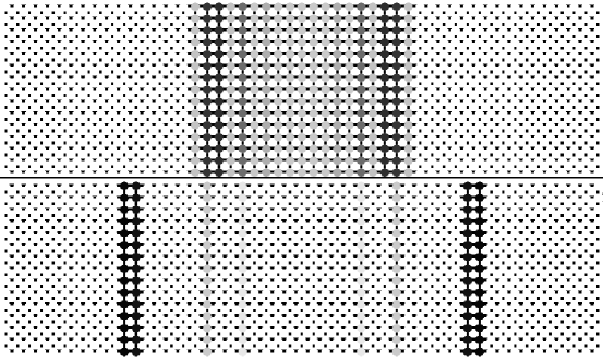
FIG. 5.: Snapshot at a subsequent time of the energy distribution for the propagation of an initial front. Upper panel: harmonic lattice. Lower panel: hard lattice.

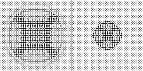
FIG. 6.: Snapshot at a subsequent time of the energy distribution for the propagation of an initial pulse at the center of the array. First panel: harmonic lattice. Second panel: hard lattice.

Typical gray-scale snapshots of the energy distribution are shown in Figs. 5 and 6, and the differences, while easily understood, are clearly dramatic. In the case of the front, the tendency of a hard lattice to propagate faster than the harmonic lattice while maintaining the energy more localized is clearly realized. The associated mean distance and dispersion that quantify the comparison are shown in Fig. 7. In the case of an initial point pulse, on the other hand, there is clearly a conflict between rapid motion and smaller dispersion – one can be realized only at the expense of the other. The latter “wins”: the pulse remains more localized in time in the hard lattice than in the harmonic. The associated mean radius is shown in Fig. 8. In the anharmonic lattice the pulse at first expands as fast as the harmonic but it essentially quickly saturates while the harmonic pulse continues to disperse.

FIG. 7.: First panel: temporal evolution of the mean distance $\langle x\rangle$ of front propagation in harmonic (solid line) and hard anharmonic (dashed line) lattices. Second panel: the associated dispersion as a function of the mean distance traveled.

FIG. 8.: Temporal evolution of the mean radius $\langle r\rangle$ of pulse propagation in harmonic (solid line) and hard anharmonic (dashed line) lattices.

V Conclusions

In this paper we have considered pulse propagation in discrete arrays of masses connected by harmonic or anharmonic springs. We have focused on the pulse velocity and width, and have found a pattern of behavior that can be strongly correlated with the energy dependence of the mean array frequency.

First we investigated the propagation of pulses in isolated (microcanonical) arrays. We found that in a hard array an amplitude increase causes a pulse to travel more rapidly and less dispersively. In a harmonic array the pulse speed and width are independent of pulse amplitude, while in a soft array a more intense pulse travels more slowly and spreads out more rapidly. These trends are a result of the fact that in a hard array the mean frequency increases with energy, in a harmonic array it is independent of energy, and in a soft array the mean frequency decreases with increasing energy. In higher dimensions these trends lead to interesting initial condition dependences that in turn may lead to apparently “opposite” behavior in different cases. Thus, for example, a front in a two-dimensional isolated hard array propagates more rapidly and more sharply than in harmonic or soft arrays, and the effect is enhanced if the front is more intense. On the other hand, a point pulse in a hard array spreads more slowly than in the others: it is not possible in this geometry to both propagate quickly and yet retain a strong localization of energy, and the latter tendency dominates the dynamics.

We then investigated the effects on pulse propagation of connecting the nonlinear chains to a heat bath (we did this only for the 1D arrays). We found that dissipative forces tend to slow down the pulse in the hard array, leave its speed unchanged in the harmonic chain, and actually speed it up in the soft array. This somewhat counterintuitive behavior is, however, fully consistent with the observation that dissipation causes a decrease in energy and hence a decrease in mean frequency in the hard case and an increase in mean frequency in the soft chain (and no change in the mean frequency of the harmonic chain). Dissipation in all cases causes a narrowing of the pulse, the effect being greatest in the soft array.

An increase in temperature has the opposite (and again at first sight perhaps somewhat counterintuitive) effect: it speeds up the pulse in the hard array, leaves it unchanged in the harmonic array, and slows it down in the soft chain. Again this behavior is consistent with the frequency vs energy trends and the fact that an increase in temperature is associated with an increase in the energy of the chain. A temperature increase in all cases causes a broadening of the pulse, the effect again being greatest in the soft array.

A Frequency vs Energy for Oscillator Chains

Consider a chain of oscillators, and let us focus on the displacement variable $x$ of a particular mass in the chain, say oscillator j, whose displacement satisfies the equation of motion

$$\frac{dx_{j}}{dt}=\pm\left(2\left[E-\sum_{n}V(x_{n}-x_{n-1})\right]-\sum_{n\neq j}p_{n}^{2}\right)^{1/2}~{}.$$ (A1)

The period of oscillation for oscillator j can be defined in analogy with Eq. (12):

$$\tau(E;\bf{x^{\prime}},\bf{p^{\prime}}) = \frac{2\pi}{\omega(E;\bf{x^{\prime}},\bf{p^{\prime}})}$$ (A2)

$$= 4\int_{0}^{x_{max}}\frac{dx_{j}}{\left(2\left[E-\sum_{n}V(x_{n}-x_{n-1})\right]-\sum_{n\neq j}p_{n}^{2}\right)^{1/2}}~{},$$ (A4)

where $\bf{x^{\prime}}$ stands for the set of all the $x$’s except $x_{j}$, and similarly for $\bf{p^{\prime}}$. The upper limit of integration $x_{max}$ depends not only on $E$ but on all the other displacements and momenta, and is the positive value of $x_{j}$ at which the denominator of the integrand vanishes. The resulting $\omega$ with all the coordinate and momentum dependences is not very useful, but it would seem reasonable to simply average over all possible values of these coordinates and momenta and thus obtain an average period. We define the average period as

$$\tau(E) \equiv \left<\tau(E;\bf{x^{\prime}},\bf{p^{\prime}})\right>$$ (A6)

$$\equiv 4\ \frac{\int\cdots\int d\bf{x^{\prime}}\int\cdots\int d\bf{p^{\prime}}\int_{0}^{x_{max}}dx_{j}\left(2\left[E-\sum_{n}V(x_{n}-x_{n-1})\right]-\sum_{n\neq j}p_{n}^{2}\right)}{\int\cdots\int d\bf{x^{\prime}}\int\cdots\int d\bf{p^{\prime}}}^{-1/2}.$$ (A8)

The limits of integration not explicitly indicated are appropriate nested relations among the variables and the energy such that the argument of the square root always remains positive. The multiple integral in the denominator covers the same integration regime and insures proper normalization for this average. Our interest lies in extracting the energy dependence - the remaining energy-independent coefficients are complicated and not important for our arguments. If the pair potentials are powers as in the single oscillator example, the scaling argument can be generalized by introducing scaled variables $z_{n}\sim(x_{n}-x_{n-1})E^{1/\alpha}$ and $u_{n}\sim p_{n}E^{1/2}$ with appropriate constants of proportionality. The limits of integration then become independent of energy and the only energy dependence arises from factoring an $E^{1/2}$ from the square root in the denominator and an $E^{1/\alpha}$ from the numerator because it contains one $z-$integration more than the denominator. The result, as before, is that

$$\tau(E)={\mathcal{B}}_{\alpha}E^{\frac{1}{\alpha}-\frac{1}{2}}$$ (A10)

with a complicated but energy-independent expression for the coefficient $\mathcal{B}_{\alpha}$, and therefore

$$\omega(E)~{}\equiv~{}\frac{2\pi}{\tau(E)}\sim E^{\frac{1}{2}-\frac{1}{\alpha}}~{}.$$ (A11)

More complicated potentials require suitable generalization of this argument, but the result in any case is that the average frequencies for the hard, harmonic, and soft chains follow the same trends as those shown in Fig. 1.

B Isolated Linear Oscillator Chain

Although linear oscillator chains are of course fully understood, it is nevertheless useful to present aspects of their behavior in the context of the present discussion.

The linear equations of motion (13) with the initial conditions (16) are easily solved:

$$x_{n}(t)={\sqrt{2\varepsilon}\over{2N+1}}\sum_{q=-N}^{N}\ {\sin(\omega_{q}t)\over\omega_{q}}\ e^{-2\pi iqn/(2N+1)}=\sqrt{2\varepsilon}\int_{0}^{t}\ J_{2n}(2\sqrt{k}\tau)d\tau$$ (B1)

where the frequencies $\omega_{q}$ obey the dispersion relation

$$\omega_{q}^{2}=4k\sin^{2}\left(\frac{2\pi q}{2N+1}\right)$$ (B2)

and where $J_{n}(z)$ denotes the Bessel function of the first kind of integer order $n$. (The energy-independence of the frequencies for the harmonic chain seen here in the $\varepsilon$-independence of the $\omega_{q}$ is prominent in our discussions throughout this paper.) The momenta are then

$$\dot{x_{n}}(t)=\sqrt{2\varepsilon}\ J_{2n}(2\sqrt{k}t).$$ (B3)

FIG. 9.: Temporal evolution of the energy $E_{n}(t)$ at several sites in a harmonic chain with force constant $k=1$ and initial momentum $p_{0}=2$.

Using a number of relations obeyed by the Bessel functions it is possible to combine these results and obtain for the local energy the simple expression

$$E_{n}(t)=\varepsilon\left[J_{2n}^{2}(2\sqrt{k}t)+\frac{1}{2}J_{2n+1}^{2}(2\sqrt{k}t)+\frac{1}{2}J_{2n-1}^{2}(2\sqrt{k}t)\right]~{}.$$ (B4)

The energy profiles for various sites are shown in Fig. 9. The $n=5$ profile (here obtained from the analytic expression (B4) also appears in Fig. 4 (there obtained by numerical integration). Note that the energy is not transported in a single absorption-emission process but rather in a series of oscillatory steps of decreasing amplitude. Our analysis in the body of the paper focuses on the first energy pulse.

FIG. 10.: First panel: Mean distance traveled by the pulse (dashed curve) and pulse maximum (solid curve) as a function of time for a harmonic chain of unit force constant. Second panel: Pulse maximum as a function of time for $k=2$ (long-dashed curve), $k=1$ (solid curve), and $k=1/2$ (short-dashed curve). The slopes of these numerically generated curves are essentially as given in the analytic expression Eq. (B6).

In Section III A we rely on $\langle x(t)\rangle$, the mean distance traveled by the pulse as a function of time, as one measure to characterize the transport properties of our arrays. An alternative measure that can be calculated analytically for the harmonic chain (but turns out to be somewhat less convenient for numerical computation) is the time-dependent site $n^{*}(t)$ at which the energy is a maximum. Because the passing energy pulse in general leaves a track behind it, one expects $n^{*}(t)\equiv x_{max}(t)$ to grow more rapidly than $\langle x(t)\rangle$. That this is indeed the case is illustrated in the first panel of Fig. 10, where both quantities are shown for a harmonic chain with unit force constant. The steps in the $x_{max}$ curve are a consequence of the discreteness of the problem. The analytic result for $n^{*}(t)$ is obtained by maximizing Eq. (B4) with respect to $n$ and is, after some manipulation, found to be the solution of the relation

$$\frac{1+\sqrt{\frac{2n-1}{2n+1}}}{4n}=\frac{J_{2n}(2\sqrt{k}t)}{2\sqrt{k}tJ_{2n-1}(2\sqrt{k}t)}~{}.$$ (B5)

Except for a very short initial transient the solution is essentially linear in time and exceedingly simple:

$$n^{*}(t)\equiv x_{max}(t)\approx\sqrt{k}t~{}.$$ (B6)

This dependence is confirmed in the second panel of Fig. 10 for three values of the force constant. The curves shown are obtained numerically, and differ from the analytic straight lines only at the very earliest times by an exceedingly small barely visible amount.

REFERENCES

- [1] E. Fermi, J. R. Pasta, and S. M. Ulam, in Collected Works of Enrico Fermi, Vol. II (University of Chicago Press, Chicago, 1965), pp.978-980; S. Lepri, R. Livi and A. Politi, Phys. Rev. Lett. 78, 1896 (1997); B. Hu, B. Li and H. Zhao, Phys. Rev. E 57, 2992 (1998); P. Allen and J. Kelner, Am. J. Phys. 66, 497 (1998); R. Bourbonnais and R. Maynard, Phys. Rev. Lett. 64, 1397 (1990); D. Visco and S. Sen, Phys. Rev. E 57, 224 (1998); S. Flach and C. R. Willis, Physics Reports 295, 181 (1998).
- [2] T. Dauxois and M. Peyrard, Phys. Rev. Lett. 70, 3935 (1993); J. Szeftel and P. Laurent, Phys. Rev. E 57, 1134 (1998); J. M. Bilbault and P. Marquié, Phys. Rev. E 53, 5403 (1996); A. J. Sievers and S. Takeno, Phys. Rev. Lett. 61, 970 (1988); K. Hori and S. Takeno, J. Phys. Soc. Japan 61, 2186 (1992); ibid 4263; S. Takeno, J. Phys. Soc. Japan 61, 2821 (1992); V. E. Zakharov, Sov. Phys. JEPT 35, 908 (1972). J. F. Lindsner, S. Chandramouli, A. R. Bulsara, M. Löcher and W. L. Ditto, Phys. Rev. Lett. 81, 5048 (1998).
- [3] G. P. Tsironis and S. Aubry, Phys. Rev. Lett. 77, 5225 (1996); J. M. Bilbault and P. Marquié, Phys. Rev. E 53, 5403 (1996); D. W. Brown, L. J. Bernstein and K. Lindenberg, Phys. Rev. E 54, 3352 (1996); K. Lindenberg, L. Bernstein and D. W. Brown, in Stochastic Dynamics, ed. by L. Schimansky-Geier and T. Peoschel (Springer Lecture Notes in Physics, Springer-Verlag, Berlin, (1997); A. Bikaki, N. K. Voulgarakis, S. Aubry, and G. P. Tsironis, Phys. Rev. E 59, 1234 (1999).
- [4] J. García-Ojalvo and J. M. Sancho, Noise in Spatially Extended Systems (Springer, New York, 1999).
- [5] K Wiesenfeld and F. Moss, Nature 373, 33 (1995); A. R. Bulsara and L. Gammaitoni, Physics Today 49, 39 (1996); L. Gammaitoni, P. Hänggi, P. Jung, and F. Marchesoni, Rev. Mod. Phys. 70, 223 (1998).
- [6] J. García-Ojalvo, A. Hernández-Machado, and J. M. Sancho, Phys. Rev. Lett. 71, 1542 (1993); A. Becker and L. Kramer, Phys. Rev. Lett. 73, 955 (1994); C. Van Den Broeck, J. M. R. Parrondo, and R. Toral, Phys. Rev. Lett. 73, 3395 (1994); C. Van den Broeck, J. M. R. Parrondo, R. Toral, and R. Kawai, Phys. Rev. E 55, 4084 (1997).
- [7] M. A. Santos and J. M. Sancho, Phys. Rev. E 59, 98 (1999).
- [8] J. F. Lindner, B. K. Meadows, W. L. Ditto, M. E. Inchiosa, and A. R. Bulsara, Phys. Rev. Lett. 75, 3 (1995); J. F. Lindner, S. Chandramouli, A. R. Bulsara, M. Locher, and W. L. Ditto, Phys. Rev. Lett. 81, 5048 (1998).
- [9] G. P. Tsironis and S. Aubry, Phys. Rev. Lett. 77, 5225 (1996).
- [10] R. Reigada, A. H. Romero, A. Sarmiento, and K. Lindenberg, J. Chem. Phys. 111, 1373 (1999).
- [11] R. Reigada, A. Sarmiento, and K. Lindenberg, in preparation.
- [12] A. B. Pippard, The Physics of Vibration Vol. 1 (Cambridge University Press, Cambridge, 1978).
- [13] T. C. Gard, Introduction to Stochastic Differential Equations, Marcel Dekker, Vol.114 of Monographs and Textbooks in Pure and Applied Mathematics (1987).
- [14] R. Toral, in Computational Field Theory and Pattern Formation, 3rd Granada Lectures in Computational Physics, Lecture Notes in Physics Vol. 448 (Springer Verlag, Berlin, 1995).