Pattern selection in a lattice of pulse-coupled oscillators

Abstract

We study spatio-temporal pattern formation in a ring of $N$ oscillators with inhibitory unidirectional pulselike interactions. The attractors of the dynamics are limit cycles where each oscillator fires once and only once. Since some of these limit cycles lead tothe same pattern, we introduce the concept of pattern degeneracy to take it into account. Moreover, we give a qualitative estimation of the volume of the basin of attraction of each pattern by means of some probabilistic arguments and pattern degeneracy, and show how are they modified as we change the value of the coupling strength. In the limit of small coupling, our estimative formula gives a perfect agreement with numerical simulations.

I Introduction

The study of the collective behavior of populations of interacting nonlinear oscillators has attracted the interest of physicists and mathematicians for many years since they can be used to modelize several chemical, biological and physical systems[3, 4]. Among them, we should mention cardiac pacemakers cells[5], integrate and fire neurons[6] and other systems made of excitable units[7]. Most of the theoretical papers that have appeared in the scientific literature deal with oscillators interacting through continuous-time couplings, allowing them to describe the system by means of coupled differential equations and apply most of the modern nonlinear dynamics techniques. More challenging from a theoretical point of view is to consider a pulse-coupling, or in other words, oscillators coupled through instantaneous interactions that take place in a very specific moment of its period. The richness of behavior of these pulse-coupled oscillatory systems includes synchronization phenomena[8], spatio-temporal pattern formation[9] (we could mention, for instance, traveling waves[11], chessboard structures[9], and periodic waves[12] ), rhythm anihilation[13], self-organized criticality[10],…

Most of the work on pattern formation has been done in mean-field models or populations of just a few oscillators. However, such restrictions do not allow to consider the effect of certain variables whose effect can be crucial for realistic systems. The specific topology of the connections or geometry of the system are some typical examples which usually induce important changes in the collective behavior of these models. Pattern formation usually takes place when oscillatory units interact in an inhibitory way, although it has also been shown that the shape of the interacting pulse, when the spike lasts for a certain amount of time, or time delays in the interactions can lead to spatio-temporal pattern formation also in the case of excitatory couplings[16, 17]. Only recently, general solutions for the general case, where the patterns existence and stability is proved, have been worked out[14, 15]. The aim of this paper is to study some pattern properties and get a quantitative estimation of the probability of pattern selection under arbitrary initial conditions or, in the language of dynamical systems, the volume of the basin of attraction of each pattern. Keeping this goal in mind, we will use the general results given in [15] where assuming a system defined on a ring the authors developed a mathematical formalism powerful enough to get analytic information of the system. Not only about the mechanisms which are responsible for synchronization and formation of spatio-temporal structures, but also, as a complement, to proof under which conditions they are stable solutions of the dynamical equations.

Despite the apparent simplicity of the model, some ring lattices of pulse-coupled oscillators are currently used to modelize certain types of cardiac arhythmias where there is an abnormally rapid heartbeat whose period is set by the time that an excitation takes to travel the circuit [18]. Moreover, there are experiments where rings of a few R15 neurons from Aplysia are constructed and stable patterns are reported [19]. Our 1d model allows us to study analytically the most simple patterns and understand their mechanisms of selection.

The structure of this paper is as follows. In Sec II we review the model introduced in [15] as well as set the notation used throughout the paper. In Section III we study some pattern properties which will be useful for, in Section IV, propose an estimation of the probability of selection of each pattern. In the last section we present our conclusions.

II The model

Our system consists in a ring of $(N+1)$ pulse-coupled oscillators. The phase of each oscillator $\phi_{i}$ evolves linearly in time

$$\frac{d\phi_{i}}{dt}=1\hskip 20.00003pt\forall i=0,\ldots,N$$ (1)

until one of them reaches the threshold value $\phi_{th}=1$. When this happens the oscillator fires and changes the state of its rightmost neighbor according to

$\displaystyle\phi_{i}\geq 1\Rightarrow\left\{\begin{array}[]{l}\phi_{i}\rightarrow 0\\ \phi_{i+1}\rightarrow\phi_{i+1}+\varepsilon\phi_{i+1}\equiv\mu\phi_{i+1}\end{array}\right.$

subjected to periodic boundary conditions, i.e. $N+1\equiv 0$, and where $\varepsilon$ denotes the strength of the coupling and $\mu=1+\varepsilon$. Where we have assumed that, from an effective point of view, the pulse-interaction between oscillators, as well as the state of each unit of the system, can be described in terms of changes in the phase, or in other words, in terms of the so called phase response curve (PRC), $\varepsilon\phi$ in our case. A PRC for a given oscillator represents the phase advance or delay as a result of receiving an external stimuli (the pulse) at different moments in the cycle of the oscillator. We will assume $\varepsilon<0$ througout the paper, as we are only interested in spatio-temporal pattern formation and $\varepsilon>0$ always leads to the globally synchronized state[15]. This linear PRC has physical sense in some situations. For instance, it shows up when we expand the non-linear PRC for the Peskin model of pacemaker cardiac cells [5] in powers of the convexity of the driving or in neuronal modelling[20]. In practice, however, this condition can be relaxed since a nonlinear PRC does not change the qualitative behavior of the model provided the number of fixed points of the dynamics is not altered. Moreover, a linear PRC has the advantage of making the system tractable from an analytical point of view.

Let us describe the notation used in the paper. The population is ordered according to the following criterion: The oscillator which fires will be always labeled as unit 0 and the rest of the population will be ordered from this unit clockwise. After the firing, the system is driven until another oscillator reaches the threshold. Then, we relabel the units such that the oscillator at $\phi=1$ is now unit number 0, and so on. This firing + driving (FD) process for $N+1$ oscillators can be described through a suitable transformation

$$\vec{\phi}^{\prime}=T_{k}(\vec{\phi})\equiv\vec{1}+{\hbox{\tenmsb M}}_{k}\vec{\phi},$$ (2)

where ${\hbox{\tenmsb M}}_{k}$ is a $N\times N$ matrix, $\vec{\phi}$ is a vector with $N$ components, $\vec{1}$ is a vector with all its components equal to one and $k$ stands for the index of the oscillator which will fire next. We call this kind of transformation a firing map, and we have to define as many firing maps as oscillators could fire, that is, index $k$ must run from $k=1$ ($\phi_{1}$ fires) to $N$ ($\phi_{N}$ fires). For example, in the $N+1=4$ oscillators case we have that the firing map corresponding to the FD process where $\phi_{2}$ is the next oscillator which do fire,

$\phi_{0}=1$	$\stackrel{{\scriptstyle\mbox{firing}}}{{\longrightarrow}}$	$0$	$\stackrel{{\scriptstyle\mbox{driving}}}{{\longrightarrow}}$	$1-\phi_{2}=\phi^{\prime}_{2}$
$\phi_{1}$	$\longrightarrow$	$\mu\phi_{1}$	$\longrightarrow$	$\mu\phi_{1}+1-\phi_{2}=\phi^{\prime}_{3}$
$\phi_{2}$	$\longrightarrow$	$\phi_{2}$	$\longrightarrow$	$1=\phi^{\prime}_{0}$
$\phi_{3}$	$\longrightarrow$	$\phi_{3}$	$\longrightarrow$	$\phi_{3}+1-\phi_{2}=\phi^{\prime}_{1}$

would be $T_{2}(\vec{\phi})$

$$\left(\begin{array}[]{c}\phi^{\prime}_{1}\\ \phi^{\prime}_{2}\\ \phi^{\prime}_{3}\end{array}\right)=\left(\begin{array}[]{c}1\\ 1\\ 1\end{array}\right)+\underbrace{\left(\begin{array}[]{ccc}0&-1&1\\ 0&-1&0\\ -\mu&-1&0\end{array}\right)}_{{\hbox{\tenmsb M}}_{2}}\left(\begin{array}[]{c}\phi_{1}\\ \phi_{2}\\ \phi_{3}\end{array}\right)$$ (3)

and so on. Once we have defined all possible firing maps for a given number of oscillators we can proceed to deal with the attractors or fixed points of the system dynamics. As has been proved in [15] these fixed points must be cycles of $N+1$ firings. We define a cycle as a sequence of consecutive firings where each oscillator fires once and only once. Mathematically, each cycle is described by means of a return map. The return map is the transformation that gives the evolution of $\vec{\phi}$ during a cycle and is the composition of all firing maps involved in the firing sequence of that cycle

$$\vec{\phi}^{\prime}=T_{c_{1}}\circ T_{c_{2}}\ldots\circ T_{c_{N+1}}(\vec{\phi})\equiv\ \vec{R}_{c}+{\hbox{\tenmsb M}}_{c}\vec{\phi},$$ (4)

where $T_{c_{i}}\circ T_{c_{j}}(\phi)$ is the usual composition operation $T_{c_{i}}(T_{c_{j}}(\phi))$ and

$\displaystyle\vec{R}_{c}=\vec{1}+\sum_{i=c_{1}}^{c_{N}}(\prod_{j=c_{1}}^{i}{\hbox{\tenmsb M}}_{j})\cdot\vec{1}\hskip 20.00003pt\mbox{and}\hskip 20.00003pt{\hbox{\tenmsb M}}_{c}=\prod_{j=c_{1}}^{c_{N+1}}{\hbox{\tenmsb M}}_{j}.$

Note that not all possible combinations of firing maps are allowed, just those ones whose indices $c_{i}$ sum $p(N+1)$ without any partial sum equal to $q(N+1)$, where $p>q$ are positive integers.

As all firing maps are linear transformations, return maps are also linear. There are $N!$ possible cycles in the $N+1$ oscillators case (all permutations of firing sequences with the initial firing oscillator $\phi_{0}$ fixed). Following our previous example, for the four oscillators case all possible firing sequences and their associated return maps are

$$A:0,1,2,3\rightarrow T_{1}\circ T_{1}\circ T_{1}\circ T_{1}$$

$$B:0,1,3,2\rightarrow T_{2}\circ T_{3}\circ T_{2}\circ T_{1}$$

$$C:0,2,1,3\rightarrow T_{1}\circ T_{2}\circ T_{3}\circ T_{2}$$

$$D:0,2,3,1\rightarrow T_{3}\circ T_{2}\circ T_{1}\circ T_{2}$$

$$E:0,3,1,2\rightarrow T_{2}\circ T_{1}\circ T_{2}\circ T_{3}$$

$$F:0,3,2,1\rightarrow T_{3}\circ T_{3}\circ T_{3}\circ T_{3}$$

Now, in order to find the attractors of the dynamics, we must solve the fixed point equation

$$\vec{\phi}_{c}^{*}=\vec{R}_{c}+\hbox{\tenmsb M}_{c}\vec{\phi}_{c}^{*},$$ (5)

for every cycle $c$. Formally,

$$\vec{\phi}_{c}^{*}=\vec{R}_{c}\cdot({\hbox{\tenmsb I}}-{\hbox{\tenmsb M}}_{c})^{-1}.$$ (6)

As was shown in [15], there are $N$ different stable solutions to the whole set of fixed point equations. Their stability is assured by the fact that $\varepsilon<0$, since it guarantees that all eigenvalues of $\hbox{\tenmsb M}_{c}$ lie inside the unit circle for all cycles $c$. In our four oscillators example these solutions are

$$\vec{\phi}_{A}^{*}= (1,\frac{3}{4+3\varepsilon},\frac{2}{4+3\varepsilon},\frac{1}{4+3\varepsilon})$$

$$\vec{\phi}_{B}^{*}=\vec{\phi}_{C}^{*}=\vec{\phi}_{D}^{*}=\vec{\phi}_{E}^{*}= (1,\frac{1}{2+\varepsilon},1,\frac{1}{2+\varepsilon})$$

$$\vec{\phi}_{F}^{*}= (1,\frac{1}{4+\varepsilon},\frac{2+\varepsilon}{4+\varepsilon},\frac{3+\varepsilon}{4+\varepsilon})$$

Which are a kind of four-oscillators traveling wave, chessboard and inverse traveling wave structures.

From now on we will label such solutions with index $m$ ($m=1...N$) since their first component always satisfy

$$\phi_{1}^{*}=\frac{m}{N+1+m\varepsilon}.$$ (7)

Therefore, in the example, we relabel patterns $\vec{\phi}_{A}^{*}$ as $m=3$, $\vec{\phi}_{B}^{*}$, $\vec{\phi}_{C}^{*}$, $\vec{\phi}_{D}^{*}$, $\vec{\phi}_{E}^{*}$ as $m=2$ and $\vec{\phi}_{F}^{*}$ as $m=1$.

Since there are $N!$ possible cycles and $N$ solutions to Eq. (7) there will be some fixed points or patterns which will appear more than once, so, we shall use $C(N+1,m)$ to characterize these degeneracies. In the example, the values of the degeneracies are $C(4,1)=C(4,3)=1$ and $C(4,2)=4$. In general, patterns which are solutions of cycle consisting in the iterative application of the same firing map (like A and F in our example) have no periodicities whereas the ones solution of mixtures of differents firing maps (B,C,D and E) have some periodic structure that are also solution of Eq. (7) for a case with less oscillators. In Fig. 1 we can visualize the solutions for $N+1=2,3$ and $4$ oscillators and realize that solution $m=2$ for the four oscillators case is a periodic composition of solution $m=1$ for the two oscillators case.

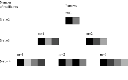
FIG. 1.: Graphic representation of the patterns solution of Eq. (7) for a small value of the coupling strength $|\varepsilon|$ at the beginning of the cycle (we must keep in mind that spatio-temporal patterns are dynamical structures that evolve in time). The leftmost square represents $\phi_{0}$ and the rightmost $\phi_{N}$, and their phase is visualized in a greyscale where black means $\phi=1$ and white $\phi=0$.

III Pattern properties

As we have seen, the stability of all patterns solution of Eq. (6) is guaranteed by the fact that $\varepsilon<0$, but the existence of such solutions is not ensured. In fact, for small values of the coupling strength $|\varepsilon|$ all patterns do exist, but, as we increase it, some patterns disappear. The reason is that the solution loses its physical meaning because $\phi_{1}^{*}>1$. Their first component is always the one that becomes larger than unity earlier and this happens, for each $m$ and according to Eq. (9), when

$$\varepsilon<\varepsilon_{m}^{*}=1-\frac{N+1}{m}.$$ (8)

Our coupling strength range of interest ends at $\varepsilon=-1$, since at $\varepsilon\leq-1$ we always find the same pathological dynamics which does not have any physical or biological sense. Realistic couplings never reach such higher values. Therefore, as $\varepsilon$ runs from $0$ to $-1$, all patterns whose $m$ satisfy $m>\frac{N+1}{2}$, disappear.

There is another interesting pattern property which has to do with the calculation of the pattern degeneracy $C(N+1,m)$. In principle, to calculate such degeneration, we should solve fixed point Eq. (6) for all possible cycles and count how many of them lead to the same pattern. Although for few oscillators the problem is quite straightforward, as we deal with higher and higher number of oscillators, the number of cycles increases (it grows as $N!$) and solving Eq. (6) becomes more difficult. Fortunately, there is another way of calculating $C(N+1,m)$ which reduces the problem to a combinatorial question. Lets show it through an example, in the previous four oscillators case, if we count, for each firing sequence, the number of oscillators which have received the pulse before firing, we can easily realize that this number is the same as its value of $m$

$$A: 0,\overline{1},\overline{2},\overline{3} \hskip 20.00003ptm=3$$

$$B: 0,\overline{1},3,\overline{2} \hskip 20.00003ptm=2$$

$$C: 0,2,\overline{1},\overline{3} \hskip 20.00003ptm=2$$

$$D: 0,2,\overline{3},\overline{1} \hskip 20.00003ptm=2$$

$$E: 0,3,\overline{1},\overline{2} \hskip 20.00003ptm=2$$

$$F: 0,3,2,\overline{1} \hskip 20.00003ptm=1$$

Here an upper bar means that the oscillator has already received a pulse during the cycle. The point is that it turns out that every pattern $m$ corresponds to a sequences of firings involving exactly $m$ oscillators that, when they do fire, had already received a pulse from their leftmost neighbor. Therefore, this property (we have checked for several values of $N+1$) allows us to associate every cycle with the pattern it leads to, just by counting these kind of firings. Now, calculating $C(N+1,m)$ becomes a straightforward matter. In Table I we have computed $C(N+1,m)$ for several values of $N+1$.

TABLE I.: Pattern degeneracy $C(N+1,m)$. First column stands for the number $N+1$ of oscillators and first row for $m$.

	1	2	3	4	5	6	7	8	9
2	1
3	1	1
4	1	4	1
5	1	11	11	1
6	1	26	66	26	1
7	1	57	302	302	57	1
8	1	120	1191	2416	1191	120	1
9	1	247	4293	15619	15619	4293	247	1
10	1	502	14608	88234	156190	88234	14608	502	1

Apart from brute force counting, degeneracy distribution $C(N+1,m)$ can also be determined from the following relation

$$C(N+1,m) = mC(N,m)+$$ (10)

$$(N+1-m)C(N,m-1),$$

for $2\leq m\leq N-1$. This recursion relation is closed by

$$C(N+1,1)=C(N+1,N)=1,$$ (11)

which correspond to the firing sequences

$\displaystyle 0,N,(N-1)...2,\overline{1}\hskip 20.00003pt\mbox{and}\hskip 20.00003pt0,\overline{1},\overline{2}...\overline{(N-1)},\overline{N},$

respectively.

From the previous relations one can deduce by induction the symmetry of the distribution with respect to its extremes at $m=1$ and $m=N$

$$C(N+1,m)=C(N+1,N+1-m),$$ (12)

and

$$\sum_{m}C(N+1,m)=N!.$$ (13)

Another interesting property is the period $\Delta_{m}^{N+1}$ of each spatio-temporal pattern $m$. Since all oscillators are in a phase-locked state, they must oscillate with the same period. Then, as the intrinsic period of each oscillator is one, and when any oscillator receives the delaying pulse from its neighbor it has a phase equal to $\phi_{1}^{*}$, one can easily realize that the effective period is

$$\Delta_{m}^{N+1}=1+\varepsilon\phi_{1}^{*}=\frac{N+1+2m\varepsilon}{N+1+m\varepsilon}.$$ (14)

Therefore, the larger the value of $m$, the longer the period of its associated pattern. It is important to notice that we have not fixed the value of such periods (each pattern has its own which is different from the others), since there are some authors who fix all periods equal to some constant, and use it as a condition to find the structures[19].

IV Pattern selection

Once we have characterized all spatio-temporal patterns, we proceed to find some general formula which give us some estimation of the probability of each pattern to be selected, or in other words, an estimation of the volume of its basin of attraction. In order to achieve this objective, we should understand the mechanism which lead to the selection of a certain spatio-temporal structure and how is it modified as the parameters of the model ($\varepsilon$ in our case) change.

There is an easy and straightforward way to get the essential features of this mechanism assuming that the probability of one oscillator to fire next is, basically, proportional to its phase (that is, if it has a phase slightly below $1$ it has a higher probability to be the next firing oscillator, whereas if it has a smaller phase, it will rarely fire next). Imagine the phases of all oscillators randomly distributed over the interval $(0,1)$. Then we let the system evolve till one of the oscillators reaches a phase $\phi_{i}=1$ and emits a pulse that is received by its rightmost neighbor which lows its phase by an amount $\varepsilon\phi_{i+1}$. Now we assume that all phases are again randomly distributed over $(0,1)$ except the one which received the pulse whose phase is distributed over $(0,1+\varepsilon)$. So, we get rid of memory effects (we know the oscillator that has fired should, now, have a phase equal to zero) and just keep in mind if each oscillator has received a pulse or has not. Therefore, the point is that under this conditions, the probability that one oscillator which has still not received a pulse do fire is some constant and, on the other hand, for the ones which had, is this constant times the factor $(1+\varepsilon)$. Then, we can characterize the probability of having some cycle just by recalling how many oscillators do fire having previously received a pulse during that cycle. Basically, this probability is proportional to $(1+\varepsilon)^{n}$ where $n$ stands for the number of oscillators which do fire having already received a pulse (the product of all constant terms will be absorbed in a normalization factor). This approach, where we assume all firings as almost-independent events, can be viewed as a kind of mean-field approximation. Then,as has been shown before, since cycles leading to the same pattern $m$ always exactly have $m$ oscillators that do fire having received the interacting pulse, we can give an estimation of the probability for pattern $m$ selection in the $N+1$ oscillators case

$$p_{m}^{N+1}(\varepsilon)\simeq{\cal N}(\varepsilon)C(N+1,m)(1+\varepsilon)^{m}.$$ (15)

Here ${\cal N}(\varepsilon)$ is chosen so that summation of the probabilities over m gives 1

$$\sum_{m}p_{m}^{N+1}(\varepsilon)=1.$$ (16)

In the limit of small coupling strength $\varepsilon\rightarrow 0$, which is the more interesting case for the majority of physical and biological systems, one can assume that interaction plays almost no role when pattern selection takes place. That is, the fact that one oscillator has received the pulse from its neighbor does not low its probability to fire as the pulse does not modify appreciably its phase. Then, we can consider that all cycles have approximately the same probability to be selected, $(1+\varepsilon)^{m}\rightarrow 1$, and only pattern degeneracy has to be considered to get a good estimation of $p_{m}^{N+1}$

$$p_{m}^{N+1}\simeq\frac{C(N+1,m)}{N!}.$$ (17)

The dominant pattern, that is, the one which has the larger probability to be selected coincides with the mean value of $m$ (due to the symmetric behavior of $C(N+1,m)$).

$$<m>_{N+1}=\sum_{m}m\frac{C(N+1,m)}{N!}=\frac{N+1}{2}.$$ (18)

For an odd number of oscillators $<m>_{N+1}$ does not exist and we have a competition between the two closest patterns $m=N/2$ and $m=(N+2)/2$. Recall that the most probable patterns turn out to be the ones with ”shortest wavelengths”, a fact that was already reported in simulations of these sort of systems[9]. In Figs. 2 and 3 we check this new approximation for the $N+1=10$ and $9$ case and realize that expected results are in good agreement with simulations data.

There also is the interesting question of how does this probability distribution modifies when the number of oscillators increases. In Fig. 4 we show $p_{m}$ for different values of $N+1$. Since there are more possible values of $m$ available, as we increase $N+1$, $p^{N+1}_{m}$ diminishes. The distribution also gets narrower as we increase $N+1$ and this becomes clear when one studies the variance of $p_{m}$. It can be found that

$$<m^{2}>_{N+1} = \sum_{m}m^{2}\frac{C(N+1,m)}{N!}$$ (19)

$$= \frac{(N+1)^{2}}{4}+\frac{N+1}{12}.$$ (20)

We could not prove this without an explicit expression for $C(N+1,m)$ but we have checked it N up to $170$. Therefore

$$\sigma^{2}_{N+1}=\frac{N+1}{12}=\frac{<m>_{N+1}}{6}.$$ (21)

It turns out that for a large number of oscillators almost all initial conditions lead to a pattern whose $m$ approximately falls in the interval $<m>_{N+1}\pm\sqrt{<m>_{N+1}}$. In order to compare it for different number of oscillators we have to normalize $m$ dividing by $N+1$. In that case, one observes that $\sigma^{2}_{N+1}\sim 1/\sqrt{N+1}$ so that as we increase $N+1$, the spread of $p^{N+1}_{m}$ diminishes getting the distribution sharpened.

FIG. 2.: Estimation of $p_{m}$ for small coupling strength in the case of an even number of oscillators $N+1=10$ and for a values of $\varepsilon$ equal to $-0.01$ and $-0.1$. Dashed line follows the theoretical values estimated through Eq. (16). We can realize that the smaller $|\varepsilon|$ is, the more accurate our estimations are. The most probable pattern is $m=(N+1)/2$ and the probability for the patterns near the extremes is almost zero due to the fast decay of $p_{m}$ there.

FIG. 3.: The same as Fig. 2 but now for an odd number of oscillators $N+1=9$. We can realize that there is not a peak anymore, instead, almost all probability is concentrated in the two competing patterns $m=N/2$ and $m=(N+2)/2$.

FIG. 4.: $p_{m}$ calculated by means of Eq. (17) for different values of $N+1$. The distribution gets narrower and the height of its peak diminishes as we increase the number of oscillators.

As Eq. (14) does not take into account the disappearance of the different patterns $m$ at the different values of $\varepsilon_{m}^{*}$ predicted by Eq. (9), it can not give a good quantitative estimation of pattern selection for higher coupling values. Nevertheless we can expand Eq. (14) to the leading order in $\varepsilon$. For small $\varepsilon$, $p_{m}^{N+1}$ are approximated by

$$p_{m}^{N+1}\simeq\frac{C(N+1,m)}{N!}(1+(m-\frac{N+1}{2})\varepsilon).$$ (22)

In Fig. 5 we compare this approximation with simulated data. The slopes near $\varepsilon=0$ do agree with Eq. (21).

FIG. 5.: Estimation of $p_{m}^{N+1}$ for a system of N+1=6 oscillators by means of the linearized Eq. (21). For small $\varepsilon$ the slopes match with simulated data.

In our simulations we calculate the probability of each pattern to be selected just by counting how many realizations (with $\phi_{0}=1$ and the rest of oscillators with random initial conditions) lead to each pattern $m$ and divide over the total number of realizations.

FIG. 6.: $p_{m}(\varepsilon)$ in the case of $N+1=4$ oscillators. In this case, we see that although for small coupling chessboard ($m=2$) is the dominant pattern, the inverse traveling wave ($m=1$) is the most probable pattern for higher values of the coupling strength. Simulations are done over 2500 realizations.

FIG. 7.: The same as Fig. 6 for $N+1=5$.

FIG. 8.: The same as Fig. 6 for $N+1=6$

Although we only have a good quantitative estimation of $p^{N+1}_{m}$ for small values of $\varepsilon$, Eq. (15) catches the two basic mechanisms responsible of pattern selection. On the one hand, it is clear that for higher values of the coupling strength $|\varepsilon|$, when one oscillator receives a pulse, it lows its phase to almost zero and, consequently, its firing probability also does. Therefore pattern selection probability $p_{m}^{N+1}(\varepsilon)$ is strongly controlled by the number of oscillators which have to fire having already received a pulse, that is, the probabilistic factor $(1+\varepsilon)^{m}$. As a consequence, $p^{N+1}_{m}$ begin to decrease sooner when $|\varepsilon|$ increases, the larger $m$ is. On the other hand, for small values of the coupling strength, interaction plays almost no role and $p_{m}^{N+1}(\varepsilon)$ is dominated by the degeneracy factor $C(N+1,m)$. Therefore $p_{m}^{N+1}(\varepsilon)$ for the different values of $m$ are basically ordered as $C(N+1,m)$. In Fig. $6$, $7$ and $8$ we show results from simulations of $p_{m}^{N+1}(\varepsilon)$ for different number of oscillators.

V Conclusions

In this paper we have studied some properties of the spatio-temporal patterns that appear in a ring of pulse-coupled oscillators with inhibitory interactions. We have focused our attention in estimating the probability of selecting a certain pattern under arbitrary initial conditions and have shown the two basic mechanisms responsible of that: the degeneracy distribution $C(N+1,m)$, for small values of $\varepsilon$, and $m$, the number of oscillators that do fire having already received a pulse, for higher values of $\varepsilon$. According to this, the different probabilities of selecting pattern $m$ start being distributed following the degeneracy distribution $C(N+1,m)$, and, as $\varepsilon$ decreases, these probabilities diminish in a hierarchical way: the larger the value of $m$, the sooner its selection probability is going to decrease, so that only patterns with smaller m will survive for higher values of $\varepsilon$. Moreover, some of the structures disappear, at the different values of $\varepsilon_{m}^{*}$, during this process. We have found out an approximation formula for $p_{m}^{N+1}(\varepsilon)$ which takes into account all these mechanisms and gives us a quantitative estimation of the different selection probabilities for small $\varepsilon$.

The estimation of the volume of the basin of attraction of each spatio-temporal pattern $m$ also gives us an idea of the stability of the different structures with respect to additive noise fluctuations (for instance, we can add some random quantity $\eta$ to all phases after each firing event or a continuous-time $\eta(t)$ in the driving). Simulations of arrays of noisy pulse coupled oscillators showed that our most probable patterns were also the most stable[9]. The present paper only concerns spatio-temporal pattern formation in a ring of oscillators, nevertheless, all results are trivially generalized to bidirectional couplings. Although the question of what happens when dealing with higher dimension lattices remains opened, some simulations results in 2d [9] showed that almost all realizations lead to a chessboard pattern in analogy with our results in the ring. That makes us believe we have caught the basic features of the problem in our 1d model.

REFERENCES

- [1] e-mail: xguardi@ffn.ub.es
- [2] e-mail: albert@ffn.ub.es
- [3] Y. Kuramoto, Chemical oscillations, waves and turbulence (Springer-Verlag, Berlin, 1984).
- [4] A.T. Winfree, The Geometry of Biological Time (Springer-Verlag, New York, 1980).
- [5] C.S. Peskin, Mathematical Aspects of Heart Physiology, Courant Institute of Mathematical Sciences, New York University, (New York) 268 (1984).
- [6] Y. Kuramoto, Physica D 50, 15 (1991)
- [7] A. Treves, Network 4, 259 (1993)
- [8] R. Mirollo and S.H. Strogatz, SIAM J. Appl. Math. 50, 1645 (1990).
- [9] A. Díaz-Guilera, A. Arenas, A. Corral, and C.J. Pérez, Physica 103D, 419 (1997).
- [10] A. Corral, C.J. Pérez, A. Díaz-Guilera, and A. Arenas, Phys. Rev. Lett. 74, 4189 (1995).
- [11] P.C Bressloff and S. Coombes, Phys. Rev. Lett. 80, 4815 (1998)
- [12] J.L. Johnson and D. Ritter, Opt. Lett. 18, 1253 (1993)
- [13] S.H. Strogatz, Nature 394, 316 (1998)
- [14] P.C Bressloff, S. Coombes and B. de Souza, Phys. Rev. Lett 79, 2791 (1997)
- [15] A. Díaz-Guilera, C.J. Pérez and A. Arenas, Phys. Rev. E 57, 3820 (1998)
- [16] C. Van Vreeswijk, L.F. Abbott and G.B.Ermentrout, J. Comp. Neurosci. 1, 313 (1994).
- [17] U. Ernst, K.Pawelzik and T.Geisel, Phys. Rev. Lett. 74, 1570 (1995)
- [18] H. Ito and L.Glass, Physica D 56, 84 (1992)
- [19] R.O. Dror, C.C. Canavier, R.J. Butera, J.W. Clark and J.H. Byrne, Biol. Cybernet. 80, 11 (1999)
- [20] C. Torras, in Statistical Mechanics of Neural Networks, ed. by L. Garrido (Springer-Verlag, Berlin, 1990), pp.65-79