Microscopic expressions for the thermodynamic temperature

Abstract

We show that arbitrary phase space vector fields can be used to generate phase functions whose ensemble averages give the thermodynamic temperature. We describe conditions for the validity of these functions in periodic boundary systems and the Molecular Dynamics (MD) ensemble, and test them with a short-ranged potential MD simulation.

I Introduction

The temperature of an equilibrium system is calculated from the mean kinetic energy of its particles. However, Rugh [1] has recently derived a new expression whose average yields the temperature in the microcanonical ensemble. The derivation involves the differentiation of the phase space volume of the ensemble (whose logarithm gives the entropy) with respect to the energy. The resultant expression depends not only on the momenta of the particles, but also on their (spatial) configuration. This result reflects the fact that the temperature of a system effects the configurations adopted by that system, and consequently one would expect to be able to calculate the temperature from configurational as well as kinetic information.

In [2], a completely configurational version of Rugh’s result was derived, and applied to Monte Carlo simulations, where the equipartition theorem cannot be used since only the configurational degrees of freedom are considered [3]. Not only did the temperature indeed correspond to the input temperature, but it was found to be a useful diagnostic for revealing coding errors as well. In [4], Rugh’s result was applied to the non-equilibrium domain, as an alternative means of defining the local temperature. As such, it correctly accounted for heat fluxes where the kinetic temperature failed to do so.

These applications have required extensions of Rugh’s original work. In this paper we will justify these modifications. We will prove that the temperature expression used in [4] is indeed equal to Rugh’s expression to $O(1/N)$, and that the configurational temperature expression given by Eq. (8) in [2] holds.

For practical reasons, atomistic simulations are usually conducted under periodic boundary conditions. Furthermore, linear momentum is conserved in molecular dynamics (MD) simulations. Thus the ensembles explored by MD simulations are not the full microcanonical or canonical ensembles, but subsets of these (the “MD ensembles”). We will therefore also prove that the temperature expressions in [2, 4] hold for periodic boundary conditions, and in the canonical and microcanonical MD ensembles.

In order to prove these results, we will derive a more general temperature expression in Sec. II. Within the framework of this broader result, we will consider which functions yield the temperature for periodic systems and MD simulations. In Sec. III we will use this theorem to obtain more specific results such as the equipartition theorem and Rugh’s result. Finally, in Sec. IV we will apply these temperature-yielding functions to MD simulations of systems with short-range potentials.

II Generalised Temperature Expressions

Let us consider an $N$-particle system at equilibrium. We define $\mathchoice{{\hbox{\boldmath$\displaystyle\Gamma$}}}{{\hbox{\boldmath$\textstyle\Gamma$}}}{{\hbox{\boldmath$\scriptstyle\Gamma$}}}{{\hbox{\boldmath$\scriptscriptstyle\Gamma$}}}=(\Gamma_{1},\ldots,\Gamma_{6N})=(p_{1},\ldots,p_{3N},q_{1},\ldots,q_{3N})$, where the $q_{i}$ and $p_{i}$ represent the $6N$ spatial coordinates and conjugate momenta which determine the dynamics of the system via Hamilton’s equations. The energy of our system is given by the Hamiltonian ${\cal H}(\mathchoice{{\hbox{\boldmath$\displaystyle\Gamma$}}}{{\hbox{\boldmath$\textstyle\Gamma$}}}{{\hbox{\boldmath$\scriptstyle\Gamma$}}}{{\hbox{\boldmath$\scriptscriptstyle\Gamma$}}})=\sum p_{i}^{2}/m+V(\{q_{j}\})$, where $V$ represents the potential energy of the system.

In this section we will prove the following result. Suppose we choose a vector field ${\mathbf{B}(\Gamma)}$ such that $0<|\left\langle\nabla{\cal H}\cdot{\mathbf{B}(\Gamma)}\right\rangle|<\infty$, $0<|\left\langle\nabla\cdot{\mathbf{B}(\Gamma)}\right\rangle|<\infty$ (where $\left\langle\ldots\right\rangle$ represents an ensemble average) and $\left\langle\nabla{\cal H}\cdot{\mathbf{B}(\Gamma)}\right\rangle$ grows more slowly than $e^{N}$ in the thermodynamic limit. Then

$$\frac{\left\langle\nabla{\cal H}\cdot{\mathbf{B}(\Gamma)}\right\rangle}{\left\langle\nabla\cdot{\mathbf{B}(\Gamma)}\right\rangle}=kT.$$ (1)

This result, as applied to the canonical ensemble, appears in [3] without proof. For certain choices of ${\mathbf{B}(\Gamma)}$, it is possible to derive such temperature expressions using the approach of Gray & Gubbins [5] — however, it is not evident how to extend their method of deriving hypervirial relations to arbitrary ${\mathbf{B}(\Gamma)}$.

In Sec. II A and II C we will prove Eq. (1) for the microcanonical and canonical ensembles respectively. Moreover, it is possible to apply Eq. (1) to systems with periodic boundary conditions and the “MD ensembles”. We will develop the additional necessary conditions in Sec. II B and II D.

A Microcanonical ensemble

We begin with a proof of Eq. (1) in the microcanonical ensemble. Consider our $N$-particle system, whose physical size is determined by a set of barriers or walls. If we denote by $\Omega$ the set of all allowed $\textstyle\Gamma$ within our phase space, then the extent of $\Omega$ in the spatial coordinates is limited by the physical size of the system. The momenta are unbounded, so that $\Omega$ forms a cylinder in phase space.

We define the surface of constant energy $A(E):=\{\mathchoice{{\hbox{\boldmath$\displaystyle\Gamma$}}}{{\hbox{\boldmath$\textstyle\Gamma$}}}{{\hbox{\boldmath$\scriptstyle\Gamma$}}}{{\hbox{\boldmath$\scriptscriptstyle\Gamma$}}}:{\cal H}(\mathchoice{{\hbox{\boldmath$\displaystyle\Gamma$}}}{{\hbox{\boldmath$\textstyle\Gamma$}}}{{\hbox{\boldmath$\scriptstyle\Gamma$}}}{{\hbox{\boldmath$\scriptscriptstyle\Gamma$}}})=E\}$, and the set of all points of equal or lower energy $\Omega(E):=\{\mathchoice{{\hbox{\boldmath$\displaystyle\Gamma$}}}{{\hbox{\boldmath$\textstyle\Gamma$}}}{{\hbox{\boldmath$\scriptstyle\Gamma$}}}{{\hbox{\boldmath$\scriptscriptstyle\Gamma$}}}:{\cal H}(\mathchoice{{\hbox{\boldmath$\displaystyle\Gamma$}}}{{\hbox{\boldmath$\textstyle\Gamma$}}}{{\hbox{\boldmath$\scriptstyle\Gamma$}}}{{\hbox{\boldmath$\scriptscriptstyle\Gamma$}}})\leq E\}$. Thus $\Omega=\Omega(\infty)$. Traditionally, the microcanonical ensemble is the set of phase points whose energy lies between $E$ and $E+\Delta E,\Delta E\ll E$, with each point being equally likely to occur. Thus our (dimensionless) partition function would be

$\displaystyle\frac{1}{h^{3N}N!}\int\limits_{\Omega(E+\Delta E)\backslash\Omega(E)}\;{\sf d}{\mathchoice{{\hbox{\boldmath$\displaystyle\Gamma$}}}{{\hbox{\boldmath$\textstyle\Gamma$}}}{{\hbox{\boldmath$\scriptstyle\Gamma$}}}{{\hbox{\boldmath$\scriptscriptstyle\Gamma$}}}},$

where $h$ is Planck’s constant. In the limit as $\Delta E\rightarrow 0$, the microcanonical ensemble of energy $E$ becomes the surface $A(E)$ with a probability distribution given by the partition function

$\displaystyle\frac{1}{h^{3N}N!}\int\limits_{\Omega}\delta({\cal H}(\mathchoice{{\hbox{\boldmath$\displaystyle\Gamma$}}}{{\hbox{\boldmath$\textstyle\Gamma$}}}{{\hbox{\boldmath$\scriptstyle\Gamma$}}}{{\hbox{\boldmath$\scriptscriptstyle\Gamma$}}})-E)\;{\sf d}{\mathchoice{{\hbox{\boldmath$\displaystyle\Gamma$}}}{{\hbox{\boldmath$\textstyle\Gamma$}}}{{\hbox{\boldmath$\scriptstyle\Gamma$}}}{{\hbox{\boldmath$\scriptscriptstyle\Gamma$}}}}=\frac{1}{h^{3N}N!}\int\limits_{A(E)}\frac{\;{\sf d}{A_{E}}}{\|\nabla{\cal H}(\mathchoice{{\hbox{\boldmath$\displaystyle\Gamma$}}}{{\hbox{\boldmath$\textstyle\Gamma$}}}{{\hbox{\boldmath$\scriptstyle\Gamma$}}}{{\hbox{\boldmath$\scriptscriptstyle\Gamma$}}})\|}=\frac{1}{h^{3N}N!}\int\limits_{A(E)}{\sf d}\mu_{E},$

where ${\sf d}{A_{E}}$ represents the infinitesimal area element on $A(E)$ at $\textstyle\Gamma$, and ${\sf d}\mu_{E}={\sf d}{A_{E}}/\|\nabla{\cal H}(\mathchoice{{\hbox{\boldmath$\displaystyle\Gamma$}}}{{\hbox{\boldmath$\textstyle\Gamma$}}}{{\hbox{\boldmath$\scriptstyle\Gamma$}}}{{\hbox{\boldmath$\scriptscriptstyle\Gamma$}}})\|$. We note immediately the dimensional inconsistency of this expression. From a physical point of view, it is necessary at this point to reduce the spatial coordinates and momenta to dimensionless units $p_{i}^{*}$ and $q_{i}^{*}$. Consequently, all functions of these coordinates will remain dimensionless, and can be converted to the appropriate units after calculation in reduced units. Physically, this is equivalent to selecting a standard basis of units by which to measure all the $p_{i}$, and all the $q_{i}$ (and consequently, the units of our resultant temperature). However, this choice of units for the $p_{i}$ and $q_{i}$ can always be made independently of each other, so that this does not present a problem in practice. Indeed, since there is no unique choice of units for converting the phase space coordinates to a reduced form, there will be infinitely many different instantaneous expressions for the temperature which will all give equivalent values in different bases of units (see, e.g., [6]). In what follows, we will assume that our $p_{i}$ and $q_{i}$ are dimensionless as required (as will be the factor $h^{3N}$).

In the surface ensemble, the entropy $S(E)$ can be defined as

$\displaystyle e^{S(E)/k}=\frac{1}{h^{3N}N!}\int\limits_{A(E)}{\sf d}\mu_{E},$

and the average value of a phase function ${\cal B}(\mathchoice{{\hbox{\boldmath$\displaystyle\Gamma$}}}{{\hbox{\boldmath$\textstyle\Gamma$}}}{{\hbox{\boldmath$\scriptstyle\Gamma$}}}{{\hbox{\boldmath$\scriptscriptstyle\Gamma$}}})$ in the ensemble is

$\displaystyle\left\langle{\cal B}(\mathchoice{{\hbox{\boldmath$\displaystyle\Gamma$}}}{{\hbox{\boldmath$\textstyle\Gamma$}}}{{\hbox{\boldmath$\scriptstyle\Gamma$}}}{{\hbox{\boldmath$\scriptscriptstyle\Gamma$}}})\right\rangle_{E}=\frac{\int_{A(E)}{\cal B}(\mathchoice{{\hbox{\boldmath$\displaystyle\Gamma$}}}{{\hbox{\boldmath$\textstyle\Gamma$}}}{{\hbox{\boldmath$\scriptstyle\Gamma$}}}{{\hbox{\boldmath$\scriptscriptstyle\Gamma$}}}){\sf d}\mu_{E}}{\int_{A(E)}{\sf d}\mu_{E}}=\frac{e^{-S(E)/k}}{h^{3N}N!}\int\limits_{A(E)}{\cal B}(\mathchoice{{\hbox{\boldmath$\displaystyle\Gamma$}}}{{\hbox{\boldmath$\textstyle\Gamma$}}}{{\hbox{\boldmath$\scriptstyle\Gamma$}}}{{\hbox{\boldmath$\scriptscriptstyle\Gamma$}}}){\sf d}\mu_{E}.$

The temperature of a microcanonical ensemble with energy $E$, temperature $T$, entropy $S$, and volume $V$ is determined via the thermodynamic relation

$$\frac{1}{T(E)}=\left.\frac{\partial S(E)}{\partial E}\right|_{V}.$$ (2)

Suppose, for an arbitrary vector field ${\mathbf{B}(\Gamma)}$, we define ${\cal B}(\mathchoice{{\hbox{\boldmath$\displaystyle\Gamma$}}}{{\hbox{\boldmath$\textstyle\Gamma$}}}{{\hbox{\boldmath$\scriptstyle\Gamma$}}}{{\hbox{\boldmath$\scriptscriptstyle\Gamma$}}})=\nabla{\cal H}(\mathchoice{{\hbox{\boldmath$\displaystyle\Gamma$}}}{{\hbox{\boldmath$\textstyle\Gamma$}}}{{\hbox{\boldmath$\scriptstyle\Gamma$}}}{{\hbox{\boldmath$\scriptscriptstyle\Gamma$}}})\cdot{\mathbf{B}(\Gamma)}$ and

$$W_{{\cal B}}(E)=e^{S_{{\cal B}}(E)/k}=\frac{1}{h^{3N}N!}\int\limits_{A(E)}{\cal B}(\mathchoice{{\hbox{\boldmath$\displaystyle\Gamma$}}}{{\hbox{\boldmath$\textstyle\Gamma$}}}{{\hbox{\boldmath$\scriptstyle\Gamma$}}}{{\hbox{\boldmath$\scriptscriptstyle\Gamma$}}})\ {\sf d}\mu_{E},$$ (3)

where we assume $0<\left\langle{\cal B}(\mathchoice{{\hbox{\boldmath$\displaystyle\Gamma$}}}{{\hbox{\boldmath$\textstyle\Gamma$}}}{{\hbox{\boldmath$\scriptstyle\Gamma$}}}{{\hbox{\boldmath$\scriptscriptstyle\Gamma$}}})\right\rangle_{E}<\infty$. From first principles,

$$h^{3N}N!\ \frac{\partial W_{{\cal B}}(E)}{\partial E} = \lim_{\delta\rightarrow 0}h^{3N}N!\ \frac{W_{{\cal B}}(E+\delta)-W_{{\cal B}}(E)}{\delta}$$

$$= \lim_{\delta\rightarrow 0}\frac{1}{\delta}\left[\int\limits_{A(E+\delta)}{\cal B}(\mathchoice{{\hbox{\boldmath$\displaystyle\Gamma$}}}{{\hbox{\boldmath$\textstyle\Gamma$}}}{{\hbox{\boldmath$\scriptstyle\Gamma$}}}{{\hbox{\boldmath$\scriptscriptstyle\Gamma$}}})\ {\sf d}\mu_{E+\delta}-\int\limits_{A(E)}{\cal B}(\mathchoice{{\hbox{\boldmath$\displaystyle\Gamma$}}}{{\hbox{\boldmath$\textstyle\Gamma$}}}{{\hbox{\boldmath$\scriptstyle\Gamma$}}}{{\hbox{\boldmath$\scriptscriptstyle\Gamma$}}})\ {\sf d}\mu_{E}\right]$$

$$= \lim_{\delta\rightarrow 0}\frac{1}{\delta}\left[\int\limits_{A(E+\delta)}{\mathbf{B}(\Gamma)}\cdot\hat{\mathbf{n}}(\mathchoice{{\hbox{\boldmath$\displaystyle\Gamma$}}}{{\hbox{\boldmath$\textstyle\Gamma$}}}{{\hbox{\boldmath$\scriptstyle\Gamma$}}}{{\hbox{\boldmath$\scriptscriptstyle\Gamma$}}})\;{\sf d}{A}_{E+\delta}-\int\limits_{A(E)}{\mathbf{B}(\Gamma)}\cdot\hat{\mathbf{n}}(\mathchoice{{\hbox{\boldmath$\displaystyle\Gamma$}}}{{\hbox{\boldmath$\textstyle\Gamma$}}}{{\hbox{\boldmath$\scriptstyle\Gamma$}}}{{\hbox{\boldmath$\scriptscriptstyle\Gamma$}}})\;{\sf d}{A}_{E}\right],$$

where $\hat{\mathbf{n}}(\mathchoice{{\hbox{\boldmath$\displaystyle\Gamma$}}}{{\hbox{\boldmath$\textstyle\Gamma$}}}{{\hbox{\boldmath$\scriptstyle\Gamma$}}}{{\hbox{\boldmath$\scriptscriptstyle\Gamma$}}})$ is a unit normal vector to the surface $A(E)$ at $\textstyle\Gamma$. We apply Gauss’ Theorem to obtain

$$h^{3N}N!\ \frac{\partial W_{{\cal B}}(E)}{\partial E} = \lim_{\delta\rightarrow 0}\frac{1}{\delta}\int\limits_{E}^{E+\delta}\int\limits_{A(\xi)}\nabla\cdot{\mathbf{B}(\Gamma)}\ \;{\sf d}{A_{\xi}}\;{\sf d}{\xi}$$

$$= \int\limits_{A(E)}\nabla\cdot{\mathbf{B}(\Gamma)}\ {\sf d}\mu_{E}.$$

Therefore it follows that

$$\frac{1}{kT_{{\cal B}}(E)}:=\frac{1}{k}\frac{\partial S_{{\cal B}}(E)}{\partial E}=\frac{\left\langle\nabla\cdot{\mathbf{B}(\Gamma)}\right\rangle_{E}}{\left\langle\nabla{\cal H}\cdot{\mathbf{B}(\Gamma)}\right\rangle_{E}}.$$ (4)

From Eq. (3), we have that $S_{{\cal B}}(E)=S(E)+k\ln\left\langle{\cal B}(\mathchoice{{\hbox{\boldmath$\displaystyle\Gamma$}}}{{\hbox{\boldmath$\textstyle\Gamma$}}}{{\hbox{\boldmath$\scriptstyle\Gamma$}}}{{\hbox{\boldmath$\scriptscriptstyle\Gamma$}}})\right\rangle_{E}$. Now, as long as $\left\langle{\cal B}(\mathchoice{{\hbox{\boldmath$\displaystyle\Gamma$}}}{{\hbox{\boldmath$\textstyle\Gamma$}}}{{\hbox{\boldmath$\scriptstyle\Gamma$}}}{{\hbox{\boldmath$\scriptscriptstyle\Gamma$}}})\right\rangle_{E}$ grows more slowly than $e^{N}$ in the thermodynamic limit, $\partial S_{{\cal B}}(E)/\partial E=\partial S(E)/\partial E$ in the thermodynamic limit (a relation we will henceforth denote as $\partial S_{{\cal B}}(E)/\partial E\simeq\partial S(E)/\partial E$). Consequently, $T_{{\cal B}}(E)\simeq T(E)$, and we recover the same result as Eq. (1). Furthermore, we may drop the condition that $\left\langle{\cal B}(\mathchoice{{\hbox{\boldmath$\displaystyle\Gamma$}}}{{\hbox{\boldmath$\textstyle\Gamma$}}}{{\hbox{\boldmath$\scriptstyle\Gamma$}}}{{\hbox{\boldmath$\scriptscriptstyle\Gamma$}}})\right\rangle_{E}$ be positive, since Eq. (4) gives the same value, whether we use $\pm\mathbf{B}(\Gamma)$.

In order to apply Gauss’ Theorem, we require that $\nabla{\cal H}$ be continuous (ie that ${\cal H}$ be differentiable) for finite energies. As far as conditions on $\mathbf{B}(\Gamma)$ are concerned, we require that $|\left\langle\nabla\cdot{\mathbf{B}(\Gamma)}\right\rangle_{E}|<\infty$, that $0<|\left\langle\nabla{\cal H}\cdot{\mathbf{B}(\Gamma)}\right\rangle_{E}|<\infty$, and that $(\ln|\left\langle\nabla{\cal H}\cdot{\mathbf{B}(\Gamma)}\right\rangle|)/N\simeq 0$. Given the dependence of $A(E)$ on the Hamiltonian, the family of vector fields ${\mathbf{B}(\Gamma)}$ that obey these criteria is not immediately obvious, and we have not attempted to develop a more general method of generating such vector fields. We simply note that the last condition allows all finite-order polynomials and bounded functions of the $p_{i}$ and $q_{i}$, as well as ratios of finite-order polynomials. However, it remains clearer from the canonical case (where the domain of integration does not depend on the Hamiltonian) whether such functions will obey the first two conditions.

B Microcanonical Periodic and MD Systems

Let us now consider the necessary changes to the proof of Eq. (4) in order for it to hold in a periodic system. For periodic systems, the extent of $\Omega$ in the spatial coordinates is no longer determined by boundary walls, but by the size and shape of the primitive cell. If the primitive cell of the periodic system is the same size and shape as the bounded system, then $\Omega$ will be the same in both cases.

The difference between the bounded and periodic systems is that particles cannot pass through the walls of the bounded system. This implies that the energy at the walls is infinite, so that our surfaces of constant energy lie entirely within $\Omega$, and do not pass through the boundary, which we denote $\partial\Omega$. This assumption is implicit in our application of Gauss’ Theorem.

In the periodic system, particles can pass through the “walls” of our primitive cell, reappearing on the other side of the cell. Therefore surfaces of constant energy can (and do) pass through $\partial\Omega$. Thus, when we use Gauss’ Theorem, our Gaussian surface consists not only of $A(E)$ and $A(E+h)$, but also all points on $\partial\Omega$ whose energies lie between $E$ and $E+h$. This extra term is of the form

$\displaystyle\lim_{h\rightarrow 0}\frac{1}{h}\left[\int\limits_{\partial\Omega(E+h)}{\mathbf{B}(\Gamma)}\cdot\hat{\mathbf{n}}(\mathchoice{{\hbox{\boldmath$\displaystyle\Gamma$}}}{{\hbox{\boldmath$\textstyle\Gamma$}}}{{\hbox{\boldmath$\scriptstyle\Gamma$}}}{{\hbox{\boldmath$\scriptscriptstyle\Gamma$}}})\;{\sf d}{A}-\int\limits_{\partial\Omega(E)}{\mathbf{B}(\Gamma)}\cdot\hat{\mathbf{n}}(\mathchoice{{\hbox{\boldmath$\displaystyle\Gamma$}}}{{\hbox{\boldmath$\textstyle\Gamma$}}}{{\hbox{\boldmath$\scriptstyle\Gamma$}}}{{\hbox{\boldmath$\scriptscriptstyle\Gamma$}}})\;{\sf d}{A}\right]=\int\limits_{\partial A(E)}{\mathbf{B}(\Gamma)}\cdot\hat{\mathbf{n}}(\mathchoice{{\hbox{\boldmath$\displaystyle\Gamma$}}}{{\hbox{\boldmath$\textstyle\Gamma$}}}{{\hbox{\boldmath$\scriptstyle\Gamma$}}}{{\hbox{\boldmath$\scriptscriptstyle\Gamma$}}})\;{\sf d}{L},$

where $\partial\Omega(E)=\partial\Omega\cap\Omega(E)$, ${\sf d}{A}$ is the volume measure on $\partial\Omega$, $\partial A(E)=\partial\Omega\cap A(E)$, and ${\sf d}{L}$ is the volume measure on $\partial A(E)$. Note that $\hat{\mathbf{n}}(\mathchoice{{\hbox{\boldmath$\displaystyle\Gamma$}}}{{\hbox{\boldmath$\textstyle\Gamma$}}}{{\hbox{\boldmath$\scriptstyle\Gamma$}}}{{\hbox{\boldmath$\scriptscriptstyle\Gamma$}}})$ does not necessarily point in the same direction as $\nabla{\cal H}(\mathchoice{{\hbox{\boldmath$\displaystyle\Gamma$}}}{{\hbox{\boldmath$\textstyle\Gamma$}}}{{\hbox{\boldmath$\scriptstyle\Gamma$}}}{{\hbox{\boldmath$\scriptscriptstyle\Gamma$}}})$, since the walls of the primitive cell are not determined by the energy surfaces. For Eq. (4) to hold in every microcanonical ensemble, we require, as a condition on ${\mathbf{B}(\Gamma)}$, that

$$\int\limits_{\partial A(E)}{\mathbf{B}(\Gamma)}\cdot\hat{\mathbf{n}}(\mathchoice{{\hbox{\boldmath$\displaystyle\Gamma$}}}{{\hbox{\boldmath$\textstyle\Gamma$}}}{{\hbox{\boldmath$\scriptstyle\Gamma$}}}{{\hbox{\boldmath$\scriptscriptstyle\Gamma$}}})\;{\sf d}{L}=0\quad\forall E.$$ (5)

To determine which functions satisfy this criterion, we consider a system where one of the particles is at one of the walls of the primitive cell [8], corresponding to a phase point $\mathchoice{{\hbox{\boldmath$\displaystyle\Gamma$}}}{{\hbox{\boldmath$\textstyle\Gamma$}}}{{\hbox{\boldmath$\scriptstyle\Gamma$}}}{{\hbox{\boldmath$\scriptscriptstyle\Gamma$}}}_{a}$. There is an equivalent system where this particle is placed on the “opposite” wall of the primitive cell, represented by $\mathchoice{{\hbox{\boldmath$\displaystyle\Gamma$}}}{{\hbox{\boldmath$\textstyle\Gamma$}}}{{\hbox{\boldmath$\scriptstyle\Gamma$}}}{{\hbox{\boldmath$\scriptscriptstyle\Gamma$}}}_{b}$. It follows that $\hat{\mathbf{n}}(\mathchoice{{\hbox{\boldmath$\displaystyle\Gamma$}}}{{\hbox{\boldmath$\textstyle\Gamma$}}}{{\hbox{\boldmath$\scriptstyle\Gamma$}}}{{\hbox{\boldmath$\scriptscriptstyle\Gamma$}}}_{a})=-\hat{\mathbf{n}}(\mathchoice{{\hbox{\boldmath$\displaystyle\Gamma$}}}{{\hbox{\boldmath$\textstyle\Gamma$}}}{{\hbox{\boldmath$\scriptstyle\Gamma$}}}{{\hbox{\boldmath$\scriptscriptstyle\Gamma$}}}_{b})$. Therefore, since $\mathchoice{{\hbox{\boldmath$\displaystyle\Gamma$}}}{{\hbox{\boldmath$\textstyle\Gamma$}}}{{\hbox{\boldmath$\scriptstyle\Gamma$}}}{{\hbox{\boldmath$\scriptscriptstyle\Gamma$}}}_{a}$ and $\mathchoice{{\hbox{\boldmath$\displaystyle\Gamma$}}}{{\hbox{\boldmath$\textstyle\Gamma$}}}{{\hbox{\boldmath$\scriptstyle\Gamma$}}}{{\hbox{\boldmath$\scriptscriptstyle\Gamma$}}}_{b}$ must lie in the same microcanonical ensemble, if ${\mathbf{B}(\Gamma}_{a})={\mathbf{B}(\Gamma}_{b})$, then the criterion of Eq. (5) is satisfied. Therefore any function which is periodic in the primitive cell [ie such that, if $\mathchoice{{\hbox{\boldmath$\displaystyle\Gamma$}}}{{\hbox{\boldmath$\textstyle\Gamma$}}}{{\hbox{\boldmath$\scriptstyle\Gamma$}}}{{\hbox{\boldmath$\scriptscriptstyle\Gamma$}}}_{a}$ and $\mathchoice{{\hbox{\boldmath$\displaystyle\Gamma$}}}{{\hbox{\boldmath$\textstyle\Gamma$}}}{{\hbox{\boldmath$\scriptstyle\Gamma$}}}{{\hbox{\boldmath$\scriptscriptstyle\Gamma$}}}_{b}$ describe the same state, then ${\mathbf{B}(\Gamma}_{a})={\mathbf{B}(\Gamma}_{b})$] will satisfy Eq. (1) for periodic systems. Note that this is a sufficient condition but not a necessary one.

Finally, let us consider the MD microcanonical ensemble. This ensemble represents the family of systems encountered during a constant energy molecular dynamics simulation, where linear momentum is conserved. Let $\Omega_{\text{MD}}$ be the set of allowed $\textstyle\Gamma$ for such a simulation. Clearly $\Omega_{\text{MD}}$ is smaller than $\Omega$, which admits all possibilities for the total linear momentum. Phase points $\textstyle\Gamma$ with the same linear momentum in the $x$-direction, say, all lie on the same (hyper)plane in $\Omega$, so that $\Omega_{\text{MD}}$ is the intersection of $\Omega$ with the three phase space planes which correspond to conservation of linear momentum in each Cartesian direction. We denote their normal vectors as $\mathbf{\hat{P}}_{x}$, $\mathbf{\hat{P}}_{y}$, and $\mathbf{\hat{P}}_{z}$.

The entropy will still correspond to the phase space volume, except that this volume is now $6N-4$ dimensional. However, we can only apply Gauss’ Theorem to the projection of the vector field ${\mathbf{B}(\Gamma)}$ onto $\Omega_{\text{MD}}$. Alternatively we must select ${\mathbf{B}(\Gamma)}$ so that it lies entirely in $\Omega_{\text{MD}}$. Such a ${\mathbf{B}(\Gamma)}$ must satisfy the condition that ${\mathbf{B}(\Gamma)}\cdot\mathbf{\hat{P}}_{\alpha}=0\quad(\alpha=x,y,z)$. In this case, Eq. (4) will generate the correct temperature in the MD ensemble.

C Canonical Ensemble

We now move on to a proof of Eq. (1) in the canonical ensemble, starting with the bounded case. We invoke Gauss’ Theorem over $\Omega(E)$ for an arbitrary vector field in phase space ${\mathbf{B}(\Gamma)}e^{-\beta{\cal H}(\mathchoice{{\hbox{\boldmath$\displaystyle\Gamma$}}}{{\hbox{\boldmath$\textstyle\Gamma$}}}{{\hbox{\boldmath$\scriptstyle\Gamma$}}}{{\hbox{\boldmath$\scriptscriptstyle\Gamma$}}})}$ (where we assume a finite, positive $\beta$), ie

$$\int\limits_{A(E)}e^{-\beta{\cal H}(\mathchoice{{\hbox{\boldmath$\displaystyle\Gamma$}}}{{\hbox{\boldmath$\textstyle\Gamma$}}}{{\hbox{\boldmath$\scriptstyle\Gamma$}}}{{\hbox{\boldmath$\scriptscriptstyle\Gamma$}}})}{\mathbf{B}(\Gamma)}\cdot\hat{\mathbf{n}}(\mathchoice{{\hbox{\boldmath$\displaystyle\Gamma$}}}{{\hbox{\boldmath$\textstyle\Gamma$}}}{{\hbox{\boldmath$\scriptstyle\Gamma$}}}{{\hbox{\boldmath$\scriptscriptstyle\Gamma$}}})\;{\sf d}{A_{E}} = \int\limits_{\Omega(E)}\nabla\cdot\left({\mathbf{B}(\Gamma)}e^{-\beta{\cal H}(\mathchoice{{\hbox{\boldmath$\displaystyle\Gamma$}}}{{\hbox{\boldmath$\textstyle\Gamma$}}}{{\hbox{\boldmath$\scriptstyle\Gamma$}}}{{\hbox{\boldmath$\scriptscriptstyle\Gamma$}}})}\right)\;{\sf d}{\Gamma}$$

$$= \int\limits_{\Omega(E)}e^{-\beta{\cal H}(\mathchoice{{\hbox{\boldmath$\displaystyle\Gamma$}}}{{\hbox{\boldmath$\textstyle\Gamma$}}}{{\hbox{\boldmath$\scriptstyle\Gamma$}}}{{\hbox{\boldmath$\scriptscriptstyle\Gamma$}}})}\nabla\cdot{\mathbf{B}(\Gamma)}\;{\sf d}{\Gamma}-\ \beta\!\!\int\limits_{\Omega(E)}e^{-\beta{\cal H}(\mathchoice{{\hbox{\boldmath$\displaystyle\Gamma$}}}{{\hbox{\boldmath$\textstyle\Gamma$}}}{{\hbox{\boldmath$\scriptstyle\Gamma$}}}{{\hbox{\boldmath$\scriptscriptstyle\Gamma$}}})}\nabla{\cal H}(\mathchoice{{\hbox{\boldmath$\displaystyle\Gamma$}}}{{\hbox{\boldmath$\textstyle\Gamma$}}}{{\hbox{\boldmath$\scriptstyle\Gamma$}}}{{\hbox{\boldmath$\scriptscriptstyle\Gamma$}}})\cdot{\mathbf{B}(\Gamma)}\;{\sf d}{\Gamma}.$$

In the limit as $E\rightarrow\infty$, we obtain

$$\lim_{E\rightarrow\infty}\ e^{-\beta E}\!\int\limits_{A(E)}{\mathbf{B}(\Gamma)}\cdot\hat{\mathbf{n}}(\mathchoice{{\hbox{\boldmath$\displaystyle\Gamma$}}}{{\hbox{\boldmath$\textstyle\Gamma$}}}{{\hbox{\boldmath$\scriptstyle\Gamma$}}}{{\hbox{\boldmath$\scriptscriptstyle\Gamma$}}})\;{\sf d}{A_{E}}=\int\limits_{\Omega}e^{-\beta{\cal H}(\mathchoice{{\hbox{\boldmath$\displaystyle\Gamma$}}}{{\hbox{\boldmath$\textstyle\Gamma$}}}{{\hbox{\boldmath$\scriptstyle\Gamma$}}}{{\hbox{\boldmath$\scriptscriptstyle\Gamma$}}})}\nabla\cdot{\mathbf{B}(\Gamma)}\;{\sf d}{\Gamma}-\beta\int\limits_{\Omega}e^{-\beta{\cal H}(\mathchoice{{\hbox{\boldmath$\displaystyle\Gamma$}}}{{\hbox{\boldmath$\textstyle\Gamma$}}}{{\hbox{\boldmath$\scriptstyle\Gamma$}}}{{\hbox{\boldmath$\scriptscriptstyle\Gamma$}}})}\nabla{\cal H}(\mathchoice{{\hbox{\boldmath$\displaystyle\Gamma$}}}{{\hbox{\boldmath$\textstyle\Gamma$}}}{{\hbox{\boldmath$\scriptstyle\Gamma$}}}{{\hbox{\boldmath$\scriptscriptstyle\Gamma$}}})\cdot{\mathbf{B}(\Gamma)}\;{\sf d}{\Gamma}.$$ (6)

For Eq. (6) to be of any use, we require that the two integrals on the right hand side be finite. For the latter integral this gives us

$\displaystyle\left|\int\limits_{\Omega}e^{-\beta{\cal H}(\mathchoice{{\hbox{\boldmath$\displaystyle\Gamma$}}}{{\hbox{\boldmath$\textstyle\Gamma$}}}{{\hbox{\boldmath$\scriptstyle\Gamma$}}}{{\hbox{\boldmath$\scriptscriptstyle\Gamma$}}})}\nabla{\cal H}(\mathchoice{{\hbox{\boldmath$\displaystyle\Gamma$}}}{{\hbox{\boldmath$\textstyle\Gamma$}}}{{\hbox{\boldmath$\scriptstyle\Gamma$}}}{{\hbox{\boldmath$\scriptscriptstyle\Gamma$}}})\cdot{\mathbf{B}(\Gamma)}\;{\sf d}{\Gamma}\right|<\infty\quad\Rightarrow\quad\lim_{E\rightarrow\infty}\int\limits_{A(E)}e^{-\beta E}{\mathbf{B}(\Gamma)}\cdot\hat{\mathbf{n}}(\mathchoice{{\hbox{\boldmath$\displaystyle\Gamma$}}}{{\hbox{\boldmath$\textstyle\Gamma$}}}{{\hbox{\boldmath$\scriptstyle\Gamma$}}}{{\hbox{\boldmath$\scriptscriptstyle\Gamma$}}})\;{\sf d}{A_{E}}=0.$

This means that whenever the last integral in Eq. (6) exists, the left hand side of Eq. (6) must be identically zero. It follows by rearrangement that

$$\frac{1}{kT}=\beta=\frac{\int\limits_{\Omega}e^{-\beta{\cal H}(\mathchoice{{\hbox{\boldmath$\displaystyle\Gamma$}}}{{\hbox{\boldmath$\textstyle\Gamma$}}}{{\hbox{\boldmath$\scriptstyle\Gamma$}}}{{\hbox{\boldmath$\scriptscriptstyle\Gamma$}}})}\nabla\cdot{\mathbf{B}(\Gamma)}\;{\sf d}{\Gamma}}{\int\limits_{\Omega}e^{-\beta{\cal H}(\mathchoice{{\hbox{\boldmath$\displaystyle\Gamma$}}}{{\hbox{\boldmath$\textstyle\Gamma$}}}{{\hbox{\boldmath$\scriptstyle\Gamma$}}}{{\hbox{\boldmath$\scriptscriptstyle\Gamma$}}})}\nabla{\cal H}(\mathchoice{{\hbox{\boldmath$\displaystyle\Gamma$}}}{{\hbox{\boldmath$\textstyle\Gamma$}}}{{\hbox{\boldmath$\scriptstyle\Gamma$}}}{{\hbox{\boldmath$\scriptscriptstyle\Gamma$}}})\cdot{\mathbf{B}(\Gamma)}\;{\sf d}{\Gamma}}=\frac{\left\langle\nabla\cdot{\mathbf{B}(\Gamma)}\right\rangle}{\left\langle\nabla{\cal H}(\mathchoice{{\hbox{\boldmath$\displaystyle\Gamma$}}}{{\hbox{\boldmath$\textstyle\Gamma$}}}{{\hbox{\boldmath$\scriptstyle\Gamma$}}}{{\hbox{\boldmath$\scriptscriptstyle\Gamma$}}})\cdot{\mathbf{B}(\Gamma)}\right\rangle},$$ (7)

in agreement with Eq. (1). Since $\beta$ is finite, we have subsumed the first two conditions on ${\mathbf{B}(\Gamma)}$ into the proof. The third is implicit in the convergence of $\left\langle\nabla{\cal H}\cdot{\mathbf{B}(\Gamma)}\right\rangle_{E}$. For Eq. (7) to hold, we require that the integral

$\displaystyle\ e^{-\beta E}\!\int\limits_{A(E)}{\mathbf{B}(\Gamma)}\cdot\hat{\mathbf{n}}(\mathchoice{{\hbox{\boldmath$\displaystyle\Gamma$}}}{{\hbox{\boldmath$\textstyle\Gamma$}}}{{\hbox{\boldmath$\scriptstyle\Gamma$}}}{{\hbox{\boldmath$\scriptscriptstyle\Gamma$}}})\;{\sf d}{A_{E}}=\ e^{\beta[TS(E)-E]}\left\langle{\cal B}(\mathchoice{{\hbox{\boldmath$\displaystyle\Gamma$}}}{{\hbox{\boldmath$\textstyle\Gamma$}}}{{\hbox{\boldmath$\scriptstyle\Gamma$}}}{{\hbox{\boldmath$\scriptscriptstyle\Gamma$}}})\right\rangle_{E}=\ e^{\beta[TS_{\cal B}(E)-E]}$

converge. When we consider that $e^{\beta[TS(E)-E]}$ also converges, but that $e^{S(E)}$ does not, we immediately obtain the third condition on $\mathbf{B}(\Gamma)$. Thus the conditions for Eq. (1) to hold in the canonical ensemble are the same as those for the microcanonical ensemble.

D Canonical Periodic and MD Ensembles

As with the microcanonical case, we must be careful in our application of Gauss’ Theorem to canonical systems with periodic boundary conditions. In analogy with the microcanonical case, our Gaussian surface consists not only of $A(E)$, but of $\partial\Omega(E)$ as well, and the left hand side of Eq. (6) becomes

$\displaystyle\lim_{E\rightarrow\infty}\int\limits_{A(E)\cup\partial\Omega(E)}e^{-\beta{\cal H}(\mathchoice{{\hbox{\boldmath$\displaystyle\Gamma$}}}{{\hbox{\boldmath$\textstyle\Gamma$}}}{{\hbox{\boldmath$\scriptstyle\Gamma$}}}{{\hbox{\boldmath$\scriptscriptstyle\Gamma$}}})}{\mathbf{B}(\Gamma)}\cdot\hat{\mathbf{n}}(\mathchoice{{\hbox{\boldmath$\displaystyle\Gamma$}}}{{\hbox{\boldmath$\textstyle\Gamma$}}}{{\hbox{\boldmath$\scriptstyle\Gamma$}}}{{\hbox{\boldmath$\scriptscriptstyle\Gamma$}}})\;{\sf d}{A_{E}}.$

We have already seen that the integral over $A(E)$ must go to zero in order for $\left\langle\nabla{\cal H}(\mathchoice{{\hbox{\boldmath$\displaystyle\Gamma$}}}{{\hbox{\boldmath$\textstyle\Gamma$}}}{{\hbox{\boldmath$\scriptstyle\Gamma$}}}{{\hbox{\boldmath$\scriptscriptstyle\Gamma$}}})\cdot{\mathbf{B}(\Gamma)}\right\rangle$ to exist, so we simply require that

$\displaystyle\int\limits_{\partial\Omega}e^{-\beta{\cal H}(\mathchoice{{\hbox{\boldmath$\displaystyle\Gamma$}}}{{\hbox{\boldmath$\textstyle\Gamma$}}}{{\hbox{\boldmath$\scriptstyle\Gamma$}}}{{\hbox{\boldmath$\scriptscriptstyle\Gamma$}}})}{\mathbf{B}(\Gamma)}\cdot\hat{\mathbf{n}}(\mathchoice{{\hbox{\boldmath$\displaystyle\Gamma$}}}{{\hbox{\boldmath$\textstyle\Gamma$}}}{{\hbox{\boldmath$\scriptstyle\Gamma$}}}{{\hbox{\boldmath$\scriptscriptstyle\Gamma$}}})\;{\sf d}{A}=0\quad\forall\beta.$

However, via the properties of the Laplace transform we have that

$\displaystyle\int\limits_{\partial\Omega}e^{-\beta{\cal H}(\mathchoice{{\hbox{\boldmath$\displaystyle\Gamma$}}}{{\hbox{\boldmath$\textstyle\Gamma$}}}{{\hbox{\boldmath$\scriptstyle\Gamma$}}}{{\hbox{\boldmath$\scriptscriptstyle\Gamma$}}})}{\mathbf{B}(\Gamma)}\cdot\hat{\mathbf{n}}(\mathchoice{{\hbox{\boldmath$\displaystyle\Gamma$}}}{{\hbox{\boldmath$\textstyle\Gamma$}}}{{\hbox{\boldmath$\scriptstyle\Gamma$}}}{{\hbox{\boldmath$\scriptscriptstyle\Gamma$}}})\;{\sf d}{A}=0\quad\forall\beta\quad\Leftrightarrow\int\limits_{\partial A(E)}{\mathbf{B}(\Gamma)}\cdot\hat{\mathbf{n}}(\mathchoice{{\hbox{\boldmath$\displaystyle\Gamma$}}}{{\hbox{\boldmath$\textstyle\Gamma$}}}{{\hbox{\boldmath$\scriptstyle\Gamma$}}}{{\hbox{\boldmath$\scriptscriptstyle\Gamma$}}})\;{\sf d}{L}=0\quad\forall E.$

Therefore the condition under which Eq. (1) will hold in all canonical ensembles is equivalent to the condition under which Eq. (1) will hold in all microcanonical ensembles. Just as in the microcanonical case, Eq. (7) will hold in the canonical ensemble as long as ${\mathbf{B}(\Gamma)}$ is periodic in $\Omega$.

Finally, we consider the canonical MD ensemble. As with the microcanonical MD ensemble, our application of Gauss’ Theorem requires that ${\mathbf{B}(\Gamma)}$ lie in $\Omega_{\text{MD}}$, so we again require that ${\mathbf{B}(\Gamma)}\cdot\mathbf{\hat{P}}_{\alpha}=0\quad(\alpha=x,y,z)$ for Eq. (7) to hold in the canonical MD ensemble.

Thus the conditions for Eq. (1) to hold for the periodic boundary system and the “MD ensembles” are the same in both the canonical and microcanonical ensembles.

III Formulae

Having proven Eq. (1) in the canonical and microcanonical ensembles, and found the conditions for it to hold in systems with periodic boundary conditions and the MD ensembles, we now demonstrate its use in generating expressions whose phase space average yields the system temperature.

If we choose ${\mathbf{B}(\Gamma)}=(0,\ldots,\Gamma_{i},\ldots,0)$, so that only the $i$-th component is non-zero, then we obtain

$$kT_{\text{equip}}=\frac{\left\langle\nabla{\cal H}(\mathchoice{{\hbox{\boldmath$\displaystyle\Gamma$}}}{{\hbox{\boldmath$\textstyle\Gamma$}}}{{\hbox{\boldmath$\scriptstyle\Gamma$}}}{{\hbox{\boldmath$\scriptscriptstyle\Gamma$}}})\cdot{\mathbf{B}(\Gamma)}\right\rangle}{\left\langle\nabla\cdot{\mathbf{B}(\Gamma)}\right\rangle}=\left\langle\Gamma_{i}\frac{\partial{\cal H}}{\partial\Gamma_{i}}\right\rangle$$ (8)

This is the familiar Generalised Equipartition Theorem. If $\Gamma_{i}$ is a momentum, then we obtain the Equipartition Theorem, $\left\langle p_{i}^{2}/m\right\rangle=kT$. If it is a coordinate, then we obtain the lesser known Clausius Virial Theorem, $\left\langle-q_{i}F_{i}\right\rangle=kT$, where $F_{i}$ is the generalised force acting on coordinate $q_{i}$ [9, 10]. We note that the Clausius Virial Theorem gives a function of coordinates only, whose average is the temperature of the system. However, the function ${\mathbf{B}(\Gamma)}\left(=\mathchoice{{\hbox{\boldmath$\displaystyle\Gamma$}}}{{\hbox{\boldmath$\textstyle\Gamma$}}}{{\hbox{\boldmath$\scriptstyle\Gamma$}}}{{\hbox{\boldmath$\scriptscriptstyle\Gamma$}}}\right)$ is not periodic in $\Omega$ in this case, so that this theorem does not hold for periodic systems. It is therefore of little use to practitioners of most MD simulations as a means of calculating the temperature.

If we select an arbitrary vector field ${\mathbf{X}(\Gamma)}$, and choose

$${\mathbf{B}(\Gamma)}=\frac{{\mathbf{X}(\Gamma)}}{\nabla{\cal H}(\mathchoice{{\hbox{\boldmath$\displaystyle\Gamma$}}}{{\hbox{\boldmath$\textstyle\Gamma$}}}{{\hbox{\boldmath$\scriptstyle\Gamma$}}}{{\hbox{\boldmath$\scriptscriptstyle\Gamma$}}})\cdot{\mathbf{X}(\Gamma)}},$$ (9)

then for all choices of ${\mathbf{X}(\Gamma)}$, ${\cal B}(\mathchoice{{\hbox{\boldmath$\displaystyle\Gamma$}}}{{\hbox{\boldmath$\textstyle\Gamma$}}}{{\hbox{\boldmath$\scriptstyle\Gamma$}}}{{\hbox{\boldmath$\scriptscriptstyle\Gamma$}}})\equiv 1$. Consequently, we obtain

$$\frac{1}{kT}=\left\langle\nabla\cdot\frac{{\mathbf{X}(\Gamma)}}{\nabla{\cal H}(\mathchoice{{\hbox{\boldmath$\displaystyle\Gamma$}}}{{\hbox{\boldmath$\textstyle\Gamma$}}}{{\hbox{\boldmath$\scriptstyle\Gamma$}}}{{\hbox{\boldmath$\scriptscriptstyle\Gamma$}}})\cdot{\mathbf{X}(\Gamma)}}\right\rangle,$$ (10)

providing this average exists. Substituting ${\mathbf{X}(\Gamma)}=\nabla{\cal H}(\mathchoice{{\hbox{\boldmath$\displaystyle\Gamma$}}}{{\hbox{\boldmath$\textstyle\Gamma$}}}{{\hbox{\boldmath$\scriptstyle\Gamma$}}}{{\hbox{\boldmath$\scriptscriptstyle\Gamma$}}})$, we obtain Rugh’s final equation [1]. Since the Hamiltonian is periodic in systems with periodic boundary conditions, ${\mathbf{B}(\Gamma)}$ will also be periodic, so that Rugh’s result holds in periodic systems. Furthermore, it satisfies the criterion for the MD ensembles, so that it can be applied to MD simulations as well.

IV Example : Simulation Application

In this section we consider the application of Eq. (1) to a simulation of a system of particles interacting with a short-range pair potential, as in [2, 4]. These simulations employ periodic boundary conditions, and as a consequence, the forces acting on a body are not correlated with the absolute positions of the particles, but only their relative positions. Thus many of the simple vector fields whose divergences are easily calculated (such as ${\mathbf{B}(\Gamma)}={\mathbf{\Gamma}}$) do not satisfy the first criterion for Eq. (1) to hold; in this case, $\left\langle\nabla{\cal H}\cdot{\mathbf{\Gamma}}\right\rangle_{E}=0$. In general, it is more difficult to find functions which are correlated with the inter-particle forces. Due to this difficulty, from this point on we restrict ourselves to choices of ${\mathbf{B}(\Gamma)}$ which are directly related to $\nabla{\cal H}$, to ensure that this condition is met.

A Theory

In systems of particles interacting with a short-range pair potential $\Phi(r)$, the Hamiltonian can be separated into a momentum contribution (the kinetic energy $K$) and a spatial contribution (the potential energy $V$), ie

$${\cal H}({\mathbf{\Gamma}})=K(\{p_{i}\})+V(\{q_{i}\})=\sum_{i=1}^{3N}\frac{p_{i}^{2}}{2m}+\sum_{i=1}^{N}\sum_{j<i}\Phi(\|\mathchoice{{\hbox{\boldmath$\displaystyle r$}}}{{\hbox{\boldmath$\textstyle r$}}}{{\hbox{\boldmath$\scriptstyle r$}}}{{\hbox{\boldmath$\scriptscriptstyle r$}}}_{ij}\|),$$ (11)

where $\mathchoice{{\hbox{\boldmath$\displaystyle r$}}}{{\hbox{\boldmath$\textstyle r$}}}{{\hbox{\boldmath$\scriptstyle r$}}}{{\hbox{\boldmath$\scriptscriptstyle r$}}}_{ij}=\mathchoice{{\hbox{\boldmath$\displaystyle r$}}}{{\hbox{\boldmath$\textstyle r$}}}{{\hbox{\boldmath$\scriptstyle r$}}}{{\hbox{\boldmath$\scriptscriptstyle r$}}}_{i}-\mathchoice{{\hbox{\boldmath$\displaystyle r$}}}{{\hbox{\boldmath$\textstyle r$}}}{{\hbox{\boldmath$\scriptstyle r$}}}{{\hbox{\boldmath$\scriptscriptstyle r$}}}_{j}$, and $\mathchoice{{\hbox{\boldmath$\displaystyle r$}}}{{\hbox{\boldmath$\textstyle r$}}}{{\hbox{\boldmath$\scriptstyle r$}}}{{\hbox{\boldmath$\scriptscriptstyle r$}}}_{i}$ is the vector describing the position of the $i$-th particle. If the potential has a continuous first derivative, then $\nabla{\cal H}$ satisfies the requirements of Gauss’ Theorem, and consequently those of our temperature expressions. Note that if we define $\mathchoice{{\hbox{\boldmath$\displaystyle r$}}}{{\hbox{\boldmath$\textstyle r$}}}{{\hbox{\boldmath$\scriptstyle r$}}}{{\hbox{\boldmath$\scriptscriptstyle r$}}}_{ij}$ as the minimum image separation of the $i$-th and $j$-th particles, then $V$ is periodic in the spatial coordinates. Thus $\nabla{\cal H}$ will be periodic as well. As a consequence, we can obtain the temperature of our system using Rugh’s expression, ie by substituting ${\mathbf{X}(\Gamma)}=\nabla{\cal H}(\mathchoice{{\hbox{\boldmath$\displaystyle\Gamma$}}}{{\hbox{\boldmath$\textstyle\Gamma$}}}{{\hbox{\boldmath$\scriptstyle\Gamma$}}}{{\hbox{\boldmath$\scriptscriptstyle\Gamma$}}})$ into Eq. (10) above.

We now make the following important observation — since $\nabla{\cal H}$ satisfies the criteria for Eq. (1) to hold in periodic boundary systems and MD ensembles, it follows that $\nabla K$ and $\nabla V$ must as well. Therefore, we would expect to be able to generate the temperature by substituting ${\mathbf{X}(\Gamma)}=\nabla K(\{p_{i}\})$ and ${\mathbf{X}(\Gamma)}=\nabla V(\{q_{i}\})$ into Eq. (10).

Since the interaction potential is short-ranged, $V$ will grow as $N$ in the thermodynamic limit. Consequently, the Hamiltonian grows as $N$ in the thermodynamic limit, and if we substitute ${\mathbf{B}(\Gamma)}=\nabla{\cal H}(\mathchoice{{\hbox{\boldmath$\displaystyle\Gamma$}}}{{\hbox{\boldmath$\textstyle\Gamma$}}}{{\hbox{\boldmath$\scriptstyle\Gamma$}}}{{\hbox{\boldmath$\scriptscriptstyle\Gamma$}}})$, ${\mathbf{B}(\Gamma)}=\nabla K(\{p_{i}\})$ and ${\mathbf{B}(\Gamma)}=\nabla V(\{q_{i}\})$ into Eq. (1), we would also expect to generate the temperature.

In this paper we will not examine the temperatures generated from the kinetic energy, since they are closely related to the equipartition temperature [Eq. (8)], and do not reveal any new results. Our interest lies in the fact that temperature expressions generated with $\nabla V(\{q_{i}\})$ contain no explicit reference to the momenta in our system, a fact which has been exploited in [2]. The temperature we obtain from substituting ${\mathbf{X}(\Gamma)}=\nabla{\cal H}(\mathchoice{{\hbox{\boldmath$\displaystyle\Gamma$}}}{{\hbox{\boldmath$\textstyle\Gamma$}}}{{\hbox{\boldmath$\scriptstyle\Gamma$}}}{{\hbox{\boldmath$\scriptscriptstyle\Gamma$}}})$ into Eq. (10) we denote by $T_{\text{norR}}$ — “nor” since it is generated using the normal vector field $\nabla{\cal H}$, and “R” since it is generated using Rugh’s prescription. In a similar manner, we denote by $T_{\text{conR}}$ the temperature we obtain from substituting ${\mathbf{X}(\Gamma)}=\nabla V(\{q_{i}\})$ — the configurational part of the Hamiltonian — into Eq. (10). When substituting these vector fields into Eq. (1), we denote the corresponding temperatures as $T_{\text{norF}}$ and $T_{\text{conF}}$, “F” denoting that we are calculating a ratio (fraction) of averages in this case.

In making the appropriate substitutions, we obtain the following expressions :

$$\frac{1}{kT_{\text{norR}}}=\left\langle\frac{\frac{3N}{m}-\sum_{i}\nabla_{i}\cdot{\mathbf{F}}_{i}}{\sum_{i}\frac{{\mathbf{p}}_{i}^{2}}{m^{2}}+{\mathbf{F}}_{i}^{2}}-\frac{2\sum_{i}\frac{{\mathbf{p}}_{i}^{2}}{m^{3}}+2\sum_{ij}{\mathbf{F}}_{i}{\mathbf{F}}_{j}:\nabla_{i}{\mathbf{F}}_{j}}{(\sum_{i}\frac{{\mathbf{p}}_{i}^{2}}{m^{2}}+{\mathbf{F}}_{i}^{2})^{2}}\right\rangle,$$ (13)

$$\frac{1}{kT_{\text{conR}}}=\left\langle\frac{-\sum_{i}\nabla_{i}\cdot{\mathbf{F}}_{i}}{\sum_{i}{\mathbf{F}}_{i}^{2}}-\frac{2\sum_{ij}{\mathbf{F}}_{i}{\mathbf{F}}_{j}:\nabla_{i}{\mathbf{F}}_{j}}{(\sum_{i}{\mathbf{F}}_{i}^{2})^{2}}\right\rangle,$$ (14)

$$\frac{1}{kT_{\text{norF}}}=\frac{\left\langle\frac{3N}{m}-\sum_{i}\nabla_{i}\cdot{\mathbf{F}}_{i}\right\rangle}{\left\langle\sum_{i}\frac{{\mathbf{p}}_{i}^{2}}{m^{2}}+{\mathbf{F}}_{i}^{2}\right\rangle},$$ (15)

$$\frac{1}{kT_{\text{conF}}}=\frac{\left\langle-\sum_{i}\nabla_{i}\cdot{\mathbf{F}}_{i}\right\rangle}{\left\langle\sum_{i}{\mathbf{F}}_{i}^{2}\right\rangle},$$ (16)

where the label $i$ refers to the particle, rather than the generalised coordinate. ${\mathbf{F}}_{i}$ represents the (vector) force acting on particle $i$, ${\mathbf{p}}_{i}$ represents its momentum, $\nabla_{i}=[\frac{\partial}{\partial x_{i}},\frac{\partial}{\partial y_{i}},\frac{\partial}{\partial z_{i}}]$, where $x_{i},y_{i}$ and $z_{i}$ refer to the Cartesian coordinates of ${\mathbf{r}}_{i}$, and $:$ represents the dyadic operator (ie for vectors $\mathbf{a},\mathbf{b}$ and matrix $\mathbf{M}$, $\mathbf{a}\mathbf{b}:\mathbf{M}=\sum_{\alpha,\beta}\mathbf{a}_{\alpha}\mathbf{b}_{\beta}\mathbf{M}_{\beta\alpha}$). Eq. (16) corresponds to the temperature expression used in [2], and Eq. (15) corresponds to the temperature expression used in [4].

If we consider the second term on the right hand side of Eqs. (13,14), the numerator increases as $N$ for a short-ranged potential (since ${\mathbf{F}}_{i}{\mathbf{F}}_{j}:\nabla_{i}{\mathbf{F}}_{j}$ will not contribute anything at large particle separations), but the denominator increases as $N^{2}$. Therefore this second term becomes negligible in the thermodynamic limit. Thus the order 1 term is contained in the first term on the right hand side of Eqs. (13,14). We will denote by $T_{\text{nor1}}$ and $T_{\text{con1}}$ the temperature calculated by the omission of these second terms respectively, ie

$$\frac{1}{kT_{\text{nor1}}}=\left\langle\frac{\frac{3N}{m}-\sum_{i}\nabla_{i}\cdot{\mathbf{F}}_{i}}{\sum_{i}{\mathbf{F}}_{i}^{2}+\frac{{\mathbf{p}}_{i}^{2}}{m^{2}}}\right\rangle,$$ (18)

$$\frac{1}{kT_{\text{con1}}}=\left\langle\frac{-\sum_{i}\nabla_{i}\cdot{\mathbf{F}}_{i}}{\sum_{i}{\mathbf{F}}_{i}^{2}}\right\rangle.$$ (19)

We expect that the temperatures given by Eqs. (13)–(19) should all be equal in the thermodynamic limit. It is therefore of interest to compare their rates of convergence to this limit, in order to ascertain the appropriateness of their use.

B Results

As an application of the above theory, we considered a three-dimensional microcanonical WCA-potential system. The WCA potential is defined as follows [11],

$$\Phi(r)=\left\{\begin{array}[]{ll}4\epsilon\left[\left(\frac{\sigma}{r}\right)^{12}-\left(\frac{\sigma}{r}\right)^{6}\right]+\epsilon,&r<2^{1/6}\sigma\\ 0,&\text{otherwise}\end{array}\right.,$$ (19)

where $\sigma$ and $\epsilon$ represent our units of length and energy respectively. This potential is continuous, has a continuous first derivative and a piecewise continuous second derivative. Due to the discontinuity in the derivative of the force, errors appear in the computed system trajectories whenever the separation between two particles crosses the $r=2^{1/6}\sigma$ boundary. However, these errors are too small, in comparison with system size errors, to affect our results. Thus, if we substitute this pair potential into Eq. (11), then we expect each of the temperatures defined in Eqs. (13)–(19) to be equal, to order $(\ln N)/N$.

Values of these six temperatures were calculated for the 3D microcanonical simulation of a periodic WCA system at various sizes $N$, reduced number densities $\rho^{*}$, and reduced total energies per particle $\bar{E}^{*}$. They were determined by the average of ten separate simulations, each of 200000 timesteps (of $\delta t^{*}=0.001$). The errors associated with each temperature were given by one third of the maximum deviation from the average over these ten runs.

The first comparison was made between systems with the same density and size, but differing energies. The values of the equipartition and normal temperatures ($T_{\text{equip}}$, $T_{\text{norR}}$, $T_{\text{norF}}$ and $T_{\text{nor1}}$) were calculated for a system of 500 particles with reduced density $\rho^{*}=0.8$, and reduced energies per particle ranging from $\bar{E}^{*}=0.8$ to $\bar{E}^{*}=2.5$. These values appear in Table I. The four temperatures agree to within 0.6–0.8% of the equipartition temperature over the range of energies shown.

The values for the three configurational temperatures match the corresponding normal temperatures to within 0.01%, ie to the number of digits shown in Table I. This can be explained in terms of the kinetic and configuration terms in the numerator and denominator of the normal temperature expressions. At high densities, the configuration terms are much larger than those contributed by the momentum terms — in two dimensions, this is typically a difference of four orders of magnitude, and in three dimensions, the difference is about six orders of magnitude. For this reason, the value of the normal temperature can be considered as a “perturbation” to the corresponding configurational temperature which has a negligible effect on our results. It is interesting to note, given this dependence on the physical structure of the system rather than on its momentum distribution, that the normal and configurational temperature expressions yield the correct temperature across the solid-liquid phase transition, despite the difference in the microscopic arrangements of atoms on either side of the transition temperature.

In Fig. 1, we compare a series of systems of fixed energy per particle ($\bar{E}^{*}=1.5$) and system size ($N=864$), but with varying densities. The discrepancy between $T_{\text{nor1}}$ and $T_{\text{norR}}$ increases when the density of the system is decreased — while $T_{\text{norR}}$ and $T_{\text{norF}}$ agree quite well with the equipartition values, $T_{\text{nor1}}$ becomes less and less reliable. However, in the thermodynamic limit, $T_{\text{nor1}}$ must converge to the other two normal temperatures. This result indicates that, while $T_{\text{nor1}}$ and $T_{\text{norR}}$ must converge towards the thermodynamic temperature, irrespective of the density, larger systems sizes are required for the same degree of convergence of $T_{\text{nor1}}$ as the density drops.

We should also note from Fig. 1 that, while $T_{\text{norR}}$ and $T_{\text{norF}}$ are indistinguishable from their configurational counterparts on the scale of the graph (and hence are not shown), the difference between $T_{\text{nor1}}$ and $T_{\text{con1}}$ becomes evident below densities of $\rho^{*}\approx 0.5$. This is a result of the drop in the number of particle interactions per timestep at lower densities. When the number of these interactions is reduced, the configurational contributions do not dominate the kinetic contributions as they do in the high density regime. Consequently, the inclusion of kinetic terms (which, by themselves would produce a value within 0.1% of the equipartition value) in $T_{\text{nor1}}$ will always correct $T_{\text{con1}}$ towards the equipartition value.

To further examine the system size dependence of our temperature expressions, we consider a single state point ($\rho^{*}=0.8,\bar{E}^{*}=1.5$), and compare the temperature expressions as a function of the number of particles in the system, ranging from $N=108$ to $N=2048$. The results of this comparison appear in Fig. 2, where the three configurational temperatures have been plotted against inverse system size. At this density, the difference between the normal temperatures and the corresponding configurational temperatures is not distinguishable on the scale of the graph for all but the 108 particle system (where the discrepancy is 0.02%), so we show only the configurational temperatures. We observe, within the errors of our calculations, the convergence of all four temperatures towards a common value. We would interpret this value as the thermodynamic temperature of a system at that state point, in the thermodynamic limit.

V Conclusion

We have derived a general functional which, given a vector field ${\mathbf{B}(\Gamma)}$ which satisfies certain broad conditions, will determine the thermodynamic temperature of an equilibrium system in the thermodynamic limit via Eq. (1). Its rate of convergence in the thermodynamic limit will be determined by the order of $\left\langle\mathbf{B}(\Gamma)\cdot\nabla{\cal H}\right\rangle$. We note, however, that if we define ${\mathbf{B}(\Gamma)}$ as per Eq. (9), then $\left\langle{\mathbf{B}(\Gamma)}\cdot\nabla{\cal H}\right\rangle\equiv 1$, and what we obtain in Eq. (1) is precisely the derivative of the logarithm of the ensemble phase space volume with respect to the energy. In the thermodynamic limit, this will yield the thermodynamic temperature $\partial S/\partial E$. However, for different ${\mathbf{B}(\Gamma)}$, the value we obtain will depend upon our sampling of phase space during the simulation, and hence the values obtained from different expressions may vary. The temperature expressions $T_{\text{norR}}$ and $T_{\text{conR}}$ fall into this category.

One practical problem that arises from the application of Eq. (1) to periodic boundary systems is the difficulty in avoiding vector fields ${\mathbf{B}(\Gamma)}$ such that $\left\langle{\mathbf{B}(\Gamma)}\cdot\nabla{\cal H}\right\rangle=0$. To circumvent this problem, we have only considered vector fields ${\mathbf{B}(\Gamma)}$ that are linear transformations of $\nabla{\cal H}$. This approach is by no means exhaustive, but serves to demonstrate one application of this theory.

It is clear from Eqs. (13)–(19) that $T_{\text{norR}}$ will be computationally more expensive than $T_{\text{nor1}}$ or $T_{\text{norF}}$ — the omitted term involves calculations which assume the intermolecular forces to have already been evaluated, thus requiring a second force loop. It is therefore of interest to determine whether these approximations to $\partial S/\partial E$ make a useful substitution for $T_{\text{norR}}$. From our results we conclude that $T_{\text{norF}}$ is more reliable than $T_{\text{nor1}}$, and in our work is a useful expression for the temperature whenever $T_{\text{norR}}$ is valid. It is for these reasons that the fractional forms ($T_{\text{norF}}$ or $T_{\text{conF}}$) appear in [2, 4].

Eq. (1) has important consequences for practitioners of non-equilibrium MD simulations, stressing the fact that the instantaneous kinetic energy per kinetic degree of freedom is not the only function whose ensemble average yields the temperature. The preference given to the kinetic energy is generally due to its ease of calculation: apart from this, there is no reason — in both equilibrium and non-equilibrium calculations — to prefer the kinetic energy expression over any other.

TABLE I.: A comparison of values of the three normal temperatures with values of the equipartition temperature, for simulations of systems with size $N=500$, reduced density $\rho^{*}=0.8$, and various reduced energies per particle $\bar{E}^{*}$. For each normal temperature, two values are reported. The first is the temperature as determined from the simulation, and the second is the discrepancy between that normal temperature and the equipartition temperature, given as a percentage of the equipartition temperature. The numbers in brackets indicate the error in the last decimal place given.

$\bar{E}^{*}$	$T_{\text{equip}}$	$T_{\text{norR}}$		$T_{\text{norF}}$		$T_{\text{nor1}}$
		abs	rel (%)	abs	rel (%)	abs	rel (%)
0.8	0.5081 (1)	0.5097 (3)	0.31	0.5090 (1)	0.19	0.5065 (3)	-0.31
1.0	0.6374 (1)	0.6389 (7)	0.24	0.6381 (4)	0.11	0.6348 (7)	-0.41
1.2	0.7679 (2)	0.7705 (4)	0.34	0.7694 (1)	0.20	0.7652 (4)	-0.35
1.5	0.9664 (2)	0.9701 (6)	0.38	0.9687 (2)	0.24	0.9631 (6)	-0.34
1.8	1.1671 (3)	1.1709 (6)	0.32	1.1694 (3)	0.20	1.1621 (6)	-0.43
2.0	1.3024 (2)	1.3060 (6)	0.28	1.3042 (3)	0.14	1.2958 (6)	-0.51
2.2	1.4386 (2)	1.4424 (9)	0.26	1.4403 (9)	0.12	1.4307 (9)	-0.55
2.5	1.6450 (2)	1.6497 (9)	0.28	1.6473 (8)	0.14	1.6359 (9)	-0.55

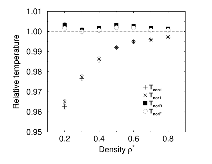
FIG. 1.: Variation of temperature values with system density. For a system of 864 particles at reduced energy per particle $\bar{E}^{*}=1.5$, various temperatures are given for different reduced densities. Temperatures are reported as a fraction of the equipartition temperature.

FIG. 2.: Variation of temperature values with system size. For the state point $\rho^{*}=0.8$, $\bar{E}^{*}=1.5$, the three configurational temperatures and the equipartition temperature are given for different system sizes.

REFERENCES

- [1] H. H. Rugh, Phys. Rev. Lett. 78, 772 (1997).
- [2] B. D. Butler, G. Ayton, O. G. Jepps, and D. J. Evans, J. Chem. Phys. 109, 6519 (1998).
- [3] M. P. Allen and D. J. Tildesley, Computer Simulation of Liquids (Clarendon Press, Oxford, 1987).
- [4] G. Ayton, O. G. Jepps, and D. J. Evans, J. Mol. Phys. 96, 915 (1999).
- [5] C. G. Gray and K. E. Gubbins, Theory of Molecular Fluids (Oxford University Press, Oxford, 1984).
- [6] G. P. Morriss and L. Rondoni, Phys. Rev. E 59, R5 (1999).
- [7] W. Rudin, Real and Complex Analysis (McGraw-Hill Book Company, Singapore, 1987).
- [8] If two or more particles are at the wall, or if the particle is in a corner, then this corresponds to a subset of of measure zero.
- [9] A. Münster, Statistical Thermodynamics, Volume I (Springer-Verlag, Heidelberg, 1969).
- [10] R. C. Tolman, The Principles of Statistical Mechanics (Dover Publications, Inc., New York, 1979).
- [11] D. J. Evans and G. P. Morriss, Statistical Mechanics of Nonequilibrium Liquids (Academic Press, London, 1990), http://rsc.anu.edu.au/~evans.