Phase–ordering dynamics of the Gay-Berne nematic liquid crystal

Abstract

Phase–ordering dynamics in nematic liquid crystals has been the subject of much active investigation in recent years in theory, experiments and simulations. With a rapid quench from the isotropic to nematic phase a large number of topological defects are formed and dominate the subsequent equilibration process. We present here the results of a molecular dynamics simulation of the Gay-Berne model of liquid crystals after such a quench in a system with 65536 molecules. Twist disclination lines as well as type-1 lines and monopoles were observed. Evidence of dynamical scaling was found in the behavior of the spatial correlation function and the density of disclination lines. However, the behavior of the structure factor provides a more sensitive measure of scaling, and we observed a crossover from a defect dominated regime at small values of the wavevector to a thermal fluctuation dominated regime at large wavevector.

I Introduction

Topological defects formed during quenches from high–temperature equilibrium phases are of interest in a wide variety of fields from condensed matter physics to cosmology [1, 2, 3, 4]. Uniaxial nematic liquid crystals are excellent materials for studying topological defects because of the variety of defects they possess and because of the ease with which they can be studied experimentally. Tables of processes involving defects, such as found in [5] are interesting both from a theoretical and from an experimental point of view. Simulations in which actual molecular configurations can be viewed and tracked could greatly elucidate these processes and aid our general understanding of defect dynamics and phase ordering. This paper represents a step towards these goals.

Simulations of defects in nematics have often used, by analogy with $O(n)$ and other model simulations [6, 7, 8], a cell-dynamical scheme [9, 10, 11] in which the order parameter $\psi$ at each site is advanced in time according to a time-dependent Ginsburg-Landau equation, within the one elastic constant approximation. Others [12, 13] have performed Monte Carlo simulations of a discretized Frank free energy, including allowance for elastic anisotropy and surface anchoring. Still others [14, 15, 16] have investigated specific types of defects or processes by directly creating the appropriate configurations as initial conditions and then evolving the system. While all of these approaches have yielded fruitful results, it would certainly be advantageous to study defects using more realistic off–lattice models with no prior bias towards forming any particular defect configurations. In this paper we present results of a simulation of a quench of the Gay–Berne nematic liquid crystal [17], a phenomenological fluid model which mimics the behavior of ellipsoidal molecules interacting through a combination of attractive and repulsive forces. This model has proven over the past decade to capture the essential physical features of real liquid crystals [18], and it is an appropriate model for studying the formation of topological defects with an off–lattice model.

This paper is organized as follows. In the next section we review the classification of nematic defects, the dynamical scaling hypothesis and the scaling forms of the real–space correlation function and structure factor. In Sec. III we present the computational details of our simulation, followed in Sec. IV by a description of our defect-finding algorithms. Our results and a comparison with theoretical predictions is presented in Sec. V, which is followed in the last section by some concluding remarks.

II Theoretical Background

A basic understanding of the defects in nematics goes back as far as the early work of Lehmann [19], but the first quantitative classification was given by Oseen[20]. Topological defect solutions are local minima of the Frank free energy

$$F=\frac{1}{2}\int d^{3}x\left[K_{11}\left({\bf\nabla\cdot\hat{n}}\right)^{2}+K_{22}\left({\bf\hat{n}\cdot\nabla\times\hat{n}}\right)^{2}+K_{33}\left|{\bf\hat{n}\times\left(\nabla\times\hat{n}\right)}\right|^{2}\right],$$ (1)

where $\bf\hat{n}$ is the nematic director. A three–dimensional uniaxial nematic has stable point (monopole) and line (disclination) defects . The former include both radial (charge +1) and hyperbolic (charge -1) geometries [21] which are topologically equivalent. Disclination line defects are either of the wedge or twist variety. Either variety is characterized by a $\pm 180^{\circ}$ director rotation about the line (i.e. the defects have charge $\pm 1/2$). A twist disclination loop is shown in Fig. 1. Note that the loop carries zero monopole charge and the director configuration is uniform at large distances from the loop. Wedge disclination loops on the other hand carry a net charge, and at large distances from them the director configuration is equivalent to that of a monopole of charge 1.

Another type of line defect is characterized by director rotations of $\pm 360^{\circ}$ (type-1 line)and is unstable to “escaping in the third dimension,” into a non-singular configuration [22] (see Fig. 2). These escaped structures can still be observed experimentally [23, 24, 25], however, and we can also visualize them in our simulation.

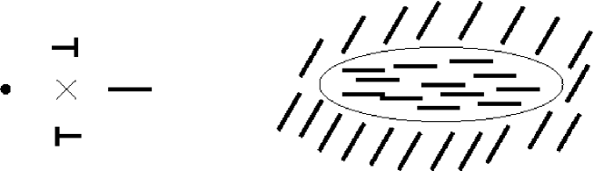
FIG. 1.: (a) Director configuration around a twist disclination line (pointing out of the page). On the left of the defect, the director is pointing out of the page, parallel to the disclination line, while on the right, the director lies in the plane of the page. Above and below the defect, the directors are depicted in intermediate orientations. (b) Illustration of the difference in director orientation between regions interior and exterior to the twist disclination line. The two regions have uniform orientations but are rotated with respect to each other by $90^{\circ}$ along an axis perpendicular to the loop.

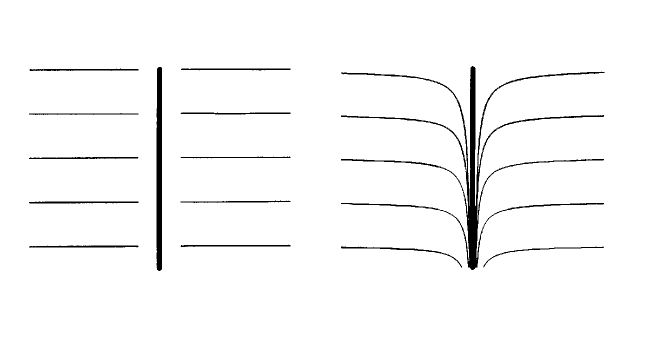
FIG. 2.: (a) Side view of a singular but unstable line with topological charge +1 (type-1line). (b) Escaped type-1line with directors tilted into a non-singular configuration.

The dynamical scaling hypothesis [26] for phase ordering processes asserts that there is a characteristic length $L(t)$ (e.g., the domain size or defect separation) such that the system appears to be time-independent (in a statistical sense) when all lengths are rescaled by $L(t)$. For nematics, theory [26] predicts that $L(t)\sim t^{1/2}$, where $t$ is the time since the ordering process began (e.g., the time since a temperature quench which leads to an isotropic–nematic transition). The disclination line density $\rho_{disc}$ (total length of disclination lines per unit volume) should then scale as $L(t)/(L(t))^{3}\sim(L(t))^{-2}\sim t^{-1}$ and the monopole density $\rho_{monop}$ (number of monopoles per unit volume) as $(L(t))^{-3}\sim t^{-3/2}$. Note that defects occur at the intersections of domains growing with differing director orientations (the Kibble mechanism [27]). Until the domains are large enough, defects are neither well-defined nor well-separated (one needs a defect separation larger than the defect core size [11]) so scaling is only assumed to hold at “late” times. Experiments are generally consistent with scaling predictions except perhaps in the behavior of monopoles [5, 28, 29]. Simulations also demonstrate scaling [9, 10, 13] but with calculated exponents somewhat different from theory and experiment. There have also been indications in simulations that more than one characteristic length may be present [10], but this is possibly just a finite-size effect.

The real-space order parameter correlation function $C({\bf r},t)$ and its Fourier transform $S({\bf k},t)$ are widely used probes [26] of domain structure and dynamical scaling. For the nematic order parameter

$$Q_{\alpha\beta}({\bf x})=\frac{3}{2}\left[{\bf\hat{u}}_{\alpha}({\bf x}){\bf\hat{u}}_{\beta}({\bf x})-\frac{1}{3}\delta_{\alpha\beta}\right],$$ (2)

one has the definitions

$$C({\bf r},t)=\frac{\int d^{d}x\ Q_{\alpha\beta}({\bf x},t)Q_{\beta\alpha}({\bf x}+{\bf r},t)}{\int d^{d}x\ Q_{\alpha\beta}({\bf x},t)Q_{\beta\alpha}({\bf x},t)},$$ (4)

$$S({\bf k},t)=\int d^{d}r\ e^{i{\bf k\cdot r}}C({\bf r},t)=\frac{Q_{\alpha\beta}({\bf k},t)Q_{\beta\alpha}({\bf-k},t)}{\int d^{d}x\ Q_{\alpha\beta}({\bf x},t)Q_{\beta\alpha}({\bf x},t)}.$$ (5)

According to the scaling hypothesis [26], the data for the orientationally averaged $C(r,t)$ at different times should collapse to a single curve when distances at time $t$ are rescaled by $L(t)$. Similarly, $S(k,t)$ should have a single, underlying scaling form: that is,

$$C(r,t)=f\left[r/L(t)\right],$$ (7)

$$S(k,t)=L^{d}g\left[kL(t)\right].$$ (8)

The late-time behavior of $S(k)$ is determined by the type and number of defects present in the system. For nematics, $S(k)$ can be written in the form [30]

$$S(k,t)=\rho_{monop}\frac{36\pi^{4}}{k^{6}}+\rho_{disc}\frac{3\pi^{3}}{k^{5}}+\frac{3}{2}\frac{k_{B}T}{Kk^{2}},$$ (9)

where the right–hand side includes contributions from the monopoles, disclinations and thermal fluctuations respectively (the nonsingular type-1 lines do not make a power–law contribution to the structure factor). Here $K$ is the elastic constant in the one-constant approximation. For thin nematic films (i.e. two spatial dimensions, but with a three–dimensional director $\bf\hat{n}$) the monopole and disclination contributions to eqn. (9) are replaced by a single contribution proportional to $k^{-4}$ arising from disclination points characterized by $\pm 180^{\circ}$ director rotations. In the three-dimensional case the disclination contribution proportional to $k^{-5}$ appears for twist and wedge disclination loops (as well as any curved disclination loop segment) at wavevectors $k\gg R^{-1}$, where $R$ is the radius of the loop [30]. For smaller wavevectors, there is no power–law contribution to the structure factor from the twist loops (recall that the director configuration is homogeneous at large distances from the loop), and wedge loops contribute a term of the same form as the monopoles. The defect contributions to the structure factor above are specific examples of Porod’s Law [26] which states that

$$S(k)\sim\rho\frac{1}{k^{2d-D}},$$ (10)

where $\rho$ is the defect density, $d$ is the number of spatial dimensions and $D$ is the defect dimensionality (e.g., points have $D=0$ and lines have $D=1$). Experiments [31] show good scaling of $S(k)$ with an asymptotic exponent approximately equal to 5, with the approach through effective exponents lying between 5 and 6 [32]. Zapotocky and Goldbart [30] have shown that such behavior would be consistent with the presence of sufficient numbers of monopoles or wedge disclination loops. However, experimentally the population of monopoles seems too low, and wedge disclinations are energetically less preferable [33, 34] than twist disclinations for typical values of the nematic elastic constants (though the former defects might be generated dynamically). From Eq. (9) we see that thermal fluctuations will dominate the structure factor for sufficiently large wavevectors satisfying $(\frac{1}{2}k_{B}T/K\rho_{disc})k^{2}>1$ (assuming that monopoles are not present in large numbers). This behavior has not been seen in the experimental studies [35, 36] carried out thus far. As discussed in [30], the scattering experiments were performed over a time range where the defect density is sufficiently large that the crossover to thermal regime is not evident for wavevectors in the visible range.

III Simulation Details

We performed a molecular dynamics (MD) simulation using the Gay-Berne model[17], an intermolecular potential similar to the simple Lennard-Jones potential but extended to model the anisotropic mesogen shape. The complete Gay-Berne potential is as follows [37]:

$$U\left({\bf\hat{u}_{i},\hat{u}_{j},\hat{r}}\right)=4\varepsilon\left({\bf\hat{u}_{i},\hat{u}_{j},\hat{r}}\right)$$

$$\times\left[\left\{\frac{\sigma_{0}}{r-\sigma\left({\bf\hat{u}_{i},\hat{u}_{j},\hat{r}}\right)+\sigma_{0}}\right\}^{12}\!-\left\{\frac{\sigma_{0}}{r-\sigma\left({\bf\hat{u}_{i},\hat{u}_{j},\hat{r}}\right)+\sigma_{0}}\right\}^{6}\right],$$ (11)

where ${\bf\hat{u}_{i},\hat{u}_{j}}$ give the orientations of the long axes of molecules $i$ and $j$, respectively, and ${\bf r}$ is the intermolecular vector (${\bf r}={\bf r_{i}}-{\bf r_{j}}$). The parameter $\sigma\left({\bf\hat{u}_{i},\hat{u}_{j},\hat{r}}\right)$ is the intermolecular separation at which the potential vanishes, and thus represents the shape of the molecules. Its explicit form is

$$\sigma\left({\bf\hat{u}_{i},\hat{u}_{j},\hat{r}}\right) = \sigma_{0}\left[1-\frac{1}{2}\chi\left\{\frac{\left({\bf\hat{r}\cdot\hat{u}_{i}}+{\bf\hat{r}\cdot\hat{u}_{j}}\right)^{2}}{1+\chi\left({\bf\hat{u}_{i}\cdot\hat{u}_{j}}\right)}\right.\right.$$ (13)

$$\left.\left.{}+\frac{\left({\bf\hat{r}\cdot\hat{u}_{i}}-{\bf\hat{r}\cdot\hat{u}_{j}}\right)^{2}}{1-\chi\left({\bf\hat{u}_{i}\cdot\hat{u}_{j}}\right)}\right\}\right]^{-1/2},$$

where $\sigma_{0}=\sigma_{s}$ (defined below) and $\chi$ is

$$\chi=\left\{\left(\sigma_{e}/\sigma_{s}\right)^{2}-1\right\}/\left\{\left(\sigma_{e}/\sigma_{s}\right)^{2}+1\right\}.$$ (14)

Here $\sigma_{e}$ is the separation between two molecules when they are oriented end-to-end, and $\sigma_{s}$ the separation when side-by-side. The well depth $\varepsilon\left({\bf\hat{u}_{i},\hat{u}_{j},\hat{r}}\right)$, representing the anisotropy of the attractive interactions, is written as

$$\varepsilon\left({\bf\hat{u}_{i},\hat{u}_{j},\hat{r}}\right)=\varepsilon_{0}\varepsilon^{\nu}\left({\bf\hat{u}_{i},\hat{u}_{j}}\right)\varepsilon^{\prime\mu}\left({\bf\hat{u}_{i},\hat{u}_{j},\hat{r}}\right),$$ (15)

where

$$\varepsilon\left({\bf\hat{u}_{i},\hat{u}_{j}}\right)=\left\{1-\chi^{2}\left({\bf\hat{u}_{i}\cdot\hat{u}_{j}}\right)^{2}\right\}^{-1/2},$$ (16)

and

$$\varepsilon^{\prime}\left({\bf\hat{u}_{i},\hat{u}_{j},\hat{r}}\right) = 1-\frac{1}{2}\chi^{\prime}\left\{\frac{\left({\bf\hat{r}\cdot\hat{u}_{i}}+{\bf\hat{r}\cdot\hat{u}_{j}}\right)^{2}}{1+\chi^{\prime}\left({\bf\hat{u}_{i}\cdot\hat{u}_{j}}\right)}\right.$$ (18)

$$\left.{}+\frac{\left({\bf\hat{r}\cdot\hat{u}_{i}}-{\bf\hat{r}\cdot\hat{u}_{j}}\right)^{2}}{1-\chi^{\prime}\left({\bf\hat{u}_{i}\cdot\hat{u}_{j}}\right)}\right\},$$

with $\chi^{\prime}$ defined in terms of $\varepsilon_{e}$ and $\varepsilon_{s}$, the end-to-end and side-by-side well depths, respectively, as

$$\chi^{\prime}=\left\{1-\left(\varepsilon_{e}/\varepsilon_{s}\right)^{1/\mu}\right\}/\left\{1+\left(\varepsilon_{e}/\varepsilon_{s}\right)^{1/\mu}\right\}.$$ (19)

The overall energy scale is set by the value of $\varepsilon_{0}$. Some representative plots of the Gay-Berne potential energy curves are shown in Fig. 3.

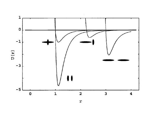
FIG. 3.: Potential energy curves for the Gay-Berne model using the parameters cited in the text. Curves are shown for four sample molecular pair configurations as indicated.

For the adjustable parameters, we used the values suggested by Berardi et al. [38]: $\mu=1,\nu=3,\sigma_{e}/\sigma_{s}=3$, and $\varepsilon_{s}/\varepsilon_{e}=5$. These values yield a nematic phase over a wider range of temperatures, compared to the original parameterization chosen by Gay and Berne [17]. The temperature was controlled by velocity rescaling [39], and the density was fixed at $\rho^{*}=0.3$ with the dimensions of the simulation box in the ratio 2:2:1. Periodic boundary conditions were applied. The system was equilibrated at $T^{*}=3.6$ in the isotropic phase for 130000 MD time steps (with a dimensionless time step of 0.004) and then a quench to $T^{*}=3.2$ was implemented (the nematic-isotropic transition temperature is approximately 3.5). The system gradually came to equilibrium in the nematic phase with the order parameter $S$ (the largest eigenvalue of $Q_{\alpha\beta}$) saturating at a value of $0.69$ over the next 100000 steps. We used a domain decomposition approach on the Cray T3E at the San Diego Supercomputing Center. Briefly, the domain decomposition approach involves dividing up the simulation volume into a number of cells, each controlled by a different processor (we used 64 cells). Because the Gay-Berne potential is short-ranged, most of the intermolecular interactions involve same-cell molecules; thus, only the relatively small number of molecules near cell boundaries will require interprocessor communications. The cell scheme and the required communications are somewhat difficult to implement, but provide very significant computational speedups. A computational scheme similar to ours is described in more detail in [40] (although we used a slightly different communication scheme in which an additional map tracking the specific subcells to be transferred between specific neighbors was implemented). We obtained timings virtually identical to those reported in the latter reference (on the order of 1 second per timestep with a 64 node partition of the Cray). Our computation time increases linearly with the number of particles and with the number of processing elements, indicating good scalability of our code.

IV Defect-Finding Methods

A preliminary step for locating defects is to break the system into a lattice of cubic bins. Note that the creation of a lattice is strictly for convenience in defect finding; the time evolution of the system allows for complete translational freedom. Even experiments, of course, have “binning” inherent in the resolution of the optical microscopy. Within each bin, the order parameter tensor $Q_{\alpha\beta}$, Eq. (2), was calculated, its largest eigenvalue taken as the local order parameter $S$ and the corresponding eigenvalue as the local director ${\bf\hat{n}}$. The bin size was chosen so that the core size of the disclinations, determined from the distance over which $S$ dropped significantly below the background value, was of the order of one lattice spacing. In our case, this resulted in a $16\times 16\times 8$ lattice, each bin holding roughly 30 molecules. It is with this lattice of orientation vectors that we began analyzing planes parallel to the $x$, $y$ and $z$ axes for the presence of defects. Note that while it is convenient to work with the orientation vectors on the lattice, we must remember that the actual directors are headless (expressing the symmetry upon rotation by 180^∘ about an axis perpendicular to the director) and so some care must be taken to account for this.

A nice method of searching for disclinations was introduced in [10] (see also [41]). Consider the directors at the corners of a square (one of the faces of a cube) in our three–dimensional lattice. The idea is to track the course of the intersections of these vectors with the order parameter sphere (actually the projective plane $RP_{2}$) as one moves around the corners of the real-space square (Fig. 4). Starting with the intersection of ${\bf\hat{n}}_{A}$ with the sphere, one then takes as the next point either the intersection of ${\bf\hat{n}}_{B}$ or $-{\bf\hat{n}}_{B}$, whichever is closest to ${\bf\hat{n}}_{A}$’s intersection. Once this point is determined, either ${\bf\hat{n}}_{C}$ or $-{\bf\hat{n}}_{C}$ is used, depending on the proximity to the previously defined point, and so on. Once the last point (from corner D) is determined, one looks at whether its intersection is in the same hemisphere as the starting point’s. If so, no defect is present—the path in order parameter space is deformable to a single point, i.e., a uniform configuration. If the first and last points are in different hemispheres, however, then a disclination line is taken to cut through the center of the square and is oriented perpendicular to the plane of the square.

To find escaped type-1 lines  we performed a similar procedure, except that we measured the actual arclength swept out as one moves from each intersection to the next. Arclengths greater than $\pi$ are counted as type-1 lines if the lattice square has not already been determined to hold a disclination (obviously, there is some overlap in the methods). The arclength $\pi$ corresponds to an escaped structure similar to that of Fig. 2 with an opening angle of about 30^∘. Experimentally, smaller opening angles are observable as type-1 lines, but smaller cutoff values of the arclength produced too many random type-1 line segments unconnected with each other or with disclinations, a situation not in accord with experiments.

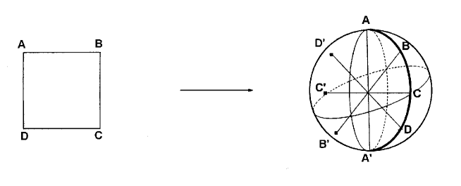
FIG. 4.: The disclination-finding algorithm. The directors at the corners of the lattice cube face shown on the left are tracked on the order parameter space sphere shown on the right. The diameters $AA^{\prime},BB^{\prime},CC^{\prime},DD^{\prime}$ correspond to the axes of the headless director at the real–space lattice sites $A,B,C,D$ respectively.

Finally, to look for monopoles, we used the method from [9]. Each of the six faces of a lattice cube is divided into two triangles and the corresponding directors are used to map out spherical triangles on the order parameter sphere. Total areas on the sphere greater than $2\pi$ are considered to be monopoles and the defect is placed at the center of the corresponding lattice cube. Note that in all these defect-finding procedures, one must be careful to apply periodic boundary conditions to the edge lattice sites.

One could also consider simulating the effect of crossed polarizers on individual planes. We used the method of [42, 43] which, phrased in the language of the Stokes parameters, uses Müller matrices to simulate the effect of a group of molecules on the polarization of incoming light. In this method, one must set values for the ordinary and extraordinary refractive indices; we used typical experimental values between 1.5 and 2 [44]. The remaining free parameter, the ratio of the thickness of the cell to the wavelength of light, was chosen to be the value which makes the calculated outgoing intensity for molecules oriented at 45^∘ to the crossed polarizer directions equal to one; we used a value of 2.5. Visualizing the resulting contour plots is aided by choosing an exponential distribution of contour values in order to sharpen the dark areas (the “brushes” [44]). This method did yield planes in which two clear brushes met at fairly well-localized points (Fig. 5), indicating the presence of a disclination  but in general, the brushes and intersections were simply not well-determined enough to be useful. We estimate that an order of magnitude increase in the number of bins (corresponding to several million Gay-Berne particles) would be required to use this crossed polarizer approach quantitatively.

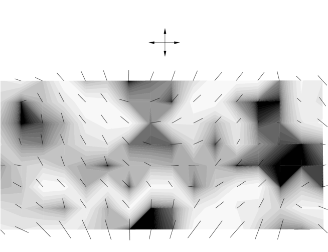
FIG. 5.: Simulated crossed-polarizer image with actual director configuration superimposed. The crossed-polarizer image is the result of applying the Müller matrix method to the single lattice plane shown. The disclination line (with topological charge 1/2) at the top-center of the image is clearly indicated by two brushes.

V Results

A Coarsening sequence

With the methods described, we observed a coarsening sequence—compare Fig. 6 with similar figures in [5]–which exhibited most of the general behaviors observed experimentally [5]. An animation of our results is available on our web site [45]. Shortly after the quench, there was a dense tangle of defect lines. This tangle gradually thinned out and we could clearly identify and follow individual defect loops. With the exception of one wedge disclination line [46] running through the sample, all of the disclination lines were of twist type (see Fig. 7) and with periodic boundary conditions formed closed loops. The presence of twist lines is consistent [33, 34] with the relative values of the elastic constants in the Gay-Berne nematic [47], namely $K_{2}<(K_{1}+K_{3})/2$. Apart from the exception mentioned above we saw no evidence for dynamically generated wedge disclination lines that might contribute substantially to the structure factor. Combination, separation and collapse of the loops were all observed. The disclination loops appeared to experience minimal center-of-mass displacement and were relatively long-lived structures. Type-1 lines took the form of single line segments or small partial loops virtually always connected to disclination line segments and often forming bridges (much like the $T$ intersections of [5]) between disclination segments from the same or distinct loops. Type-1 lines tended to fluctuate on much shorter time scales than disclinations, which seems reasonable given that the former are not topologically stable. One interesting observation is that type-1 lines often appeared as precursors to or remnants of the motion of disclination line segments. For example, the appearance of a type-1 line or several connected lines jutting out from a disclination was often followed by a kink or bend developing in the disclination line at that point. Similarly, the removal of kinks or bends often left behind type-1 lines for some period of time. The type-1 lines seemed to be initially defining and afterwards retaining a memory of the disclination path. Also, the emergence of distinct disclination loops from localized tangles often included the breaking of numerous type-1 “bonds” between the loops.

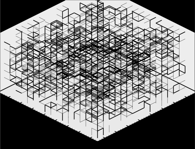
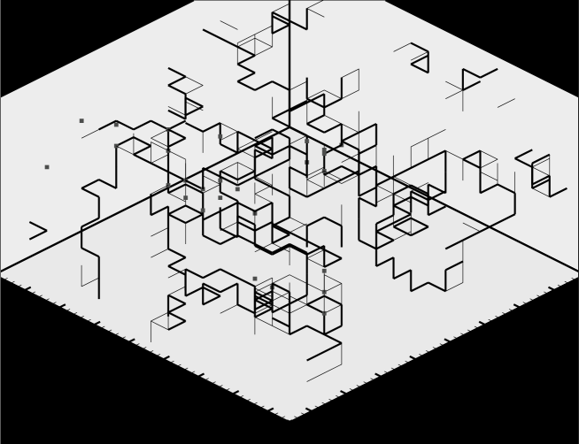
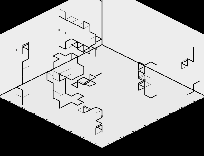
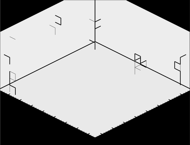
FIG. 6.: Coarsening sequence at times (a) $t=2$, (b) $t=14$, (c) $t=25$, and (d) $t=37$, with $t=0$ corresponding to the instantaneous temperature quench from the isotropic to the nematic phase. Filled squares represent point defects, thin lines represent type-1 lines and thick lines (for emphasis) represent disclinations. Note that with periodic boundary conditions, all disclination lines form closed loops. An animation of the coarsening sequence is available on our web site [45].

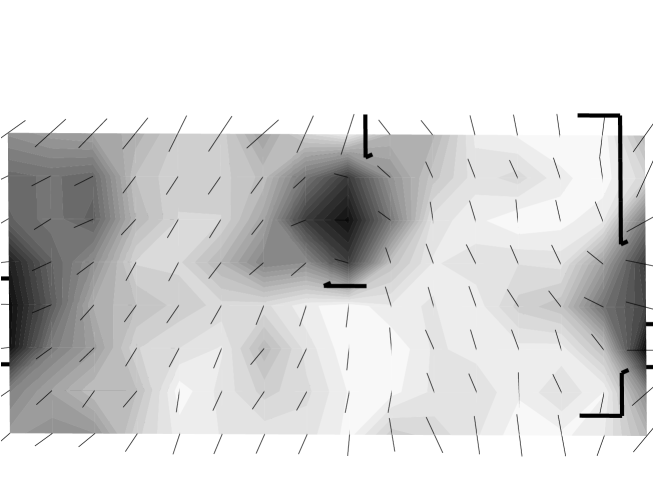
FIG. 7.: Indication of a twist disclination. A single lattice plane of directors is shown with disclinations indicated as thick lines. Dark areas indicate local directors perpendicular to the global director (along the vertical axis) while light areas indicate parallel orientations. The dark region in the center of the figure falls inside a disclination loop, clearly indicating a twist disclination. Compare with Fig. 1(b).

The monopoles we observed fluctuated even more rapidly than the type-1 lines, although in many cases, their positions remained constant, on average, over relatively longer times. Because of their fluctuations, it is difficult to make any reliable statements about specific monopole behaviors such as monopole-antimonopole annihilation, for example. We never observed monopole formation upon disclination loop collapse, a result consistent with the presence of only twist disclination loops. All of the above processes are best observed in the animations we provide on our web site [45]. The total line length of disclination lines and type-1 lines as well as the number of monopoles is plotted in Fig. 8 as a function of time. The total number of disclination loops is plotted as a function of time in Fig. 9.

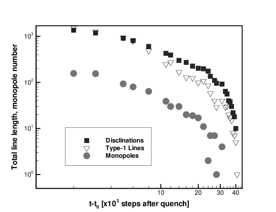
FIG. 8.: Time behavior of the various defect quantities: total length of disclination lines and type-1 lines and total number of monopoles.

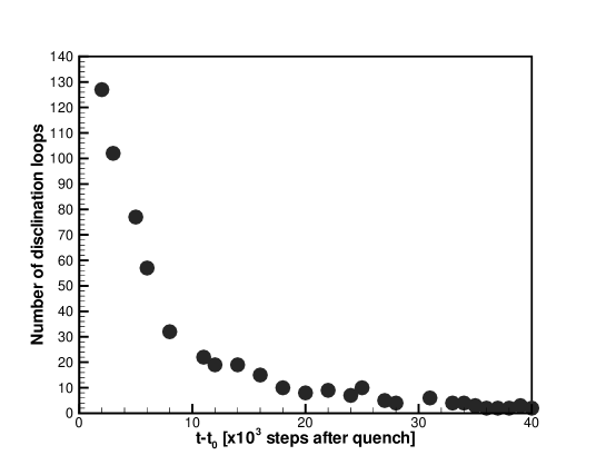
FIG. 9.: Number of disclination loops as a function of time.

B Real–space correlation function $C(r,t)$

To calculate the correlation function $C(r,t)$, Eq. (4), we reduced our bin dimensions by a factor of 2 (yielding a $32\times 32\times 16$ lattice size) to obtain a larger data set. We obtained curves for $C(r,t)$ at times spanning the entire coarsening process. Motivated by the dynamical scaling hypothesis Eq. (7) we attempted to collapse our data to a single curve with appropriate rescaling of distances. From $t=13$ (in units of thousands of steps since the temperature quench) until $t=40$ when nearly all of the defects disappeared, the $C(r,t)$ curves for different times collapse to a single curve (Fig. 11 (a)) upon rescaling distances by a length scale $L(t)$ chosen so that $C(r=L(t),t)=1/2$. This particular choice $L(t)$ for the characteristic length scale was first suggested in [10], and is the most accurate to implement numerically. The time dependence of $L(t)$ is shown in Fig. 11(b). Our system is not large enough to extract a reliable power–law for the growth of $L(t)$. However, according to the dynamic scaling hypothesis the length $L(t)$ defined by the above criterion should differ at most by prefactors or subdominant contributions at late times from other characteristic length scales of the system. For example, as we noted in Sec. II the disclination line density should scale as $(L(t))^{-2}$. In Fig. 10 we plot the disclination line density as a function of $L(t)$, over the range of times ($t=13$ to $t=40$) where we found good scaling of $C(r,t)$. A least squares fit yields an exponent $1.99\pm 0.23$, consistent with dynamical scaling. However, the range of times over which coarsening occurs is too limited (due to the small system size) to allow us to fully assess the validity of the dynamical scaling hypothesis. Similarly, while the collapse of the correlation function data to a single scaling curve is consistent with the predictions of dynamical scaling, the range of distances and times is too limited to provide more definitive support for the hypothesis. Furthermore, as we discuss in the next section when we examine the structure factor dynamical scaling may in fact be breaking down in the range $(r/L(t))<1$, even though this is not evident from the scale of the plot of $C(r,t)$.

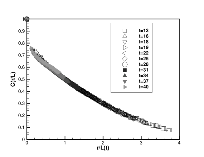
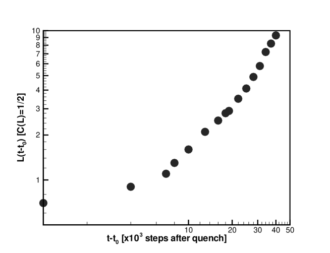
FIG. 10.: Log-log plot of disclination line density (line length per unit volume) versus the characteristic length $L$ shown in Fig. 11(b). The straight line is a least squares fit with slope $-1.99\pm 0.23$. The range of $L$ shown corresponds to the time range $t=13$ to $t=40$ where scaling behavior of $C(r,t)$ is observed as shown in Fig. 11(a).

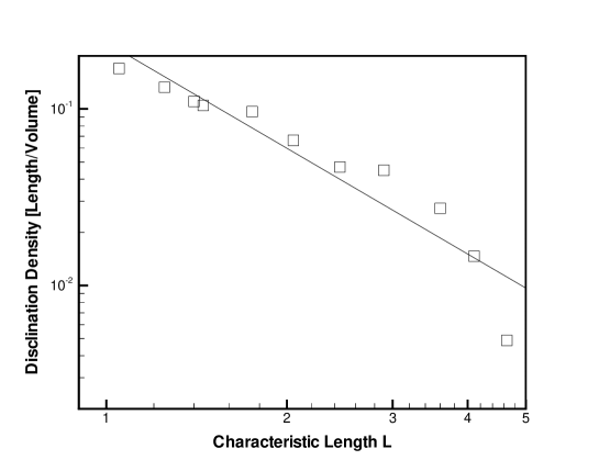
FIG. 11.: a) Correlation function $C(r,t)$ for times ranging from $t=13$ to $t=40$ with distances rescaled by the characteristic lengths defined by $C(r=L(t))=1/2$. (b) Time behavior of the characteristic length $L(t)$. Note that the data in this figure was obtained by using a smaller bin size (corresponding to a $32\times 32\times 16$ lattice) than the previous figures.

C Structure factor $S(k,t)$

We computed the structure factor $S(k,t)$, Eq.(5), by first evaluating the Fourier transform of the nematic order parameter, Eq. (2):

$$Q_{\alpha\beta}({\bf k})=\frac{V}{N}\sum_{i}\frac{3}{2}\left[{\bf\hat{u}}_{i\alpha}{\bf\hat{u}}_{i\beta}-\frac{1}{3}\delta_{\alpha\beta}\right]\exp(i{\bf k\cdot r}),$$ (20)

where $V$ and $N$ are the system volume and number of molecules respectively. As in Sec. V B we used a $32\times 32\times 16$ lattice. The wavevectors ${\bf k}$ have components which are multiples of the minimum values commensurate with the MD cell sizes in each direction. Motivated by the expression Eq. (8) for the structure factor we plotted our results in log–log form. Representative results are shown in Figs. 12, 13 and 14, where we have computed $S(k)$ for values of $k\geq 2\pi/16$, the minimum commensurate value along the shortest dimension of the cell, and less than $k\simeq 2$. For values of $k$ larger than 2 we are unable to fit our data to the long wavelength expression Eq. (5) for $S(k)$. Fig. 12 corresponds to time $t=27$ when there are still a sizable number of defects, Fig. 13 corresponds to $t=40$ near the end of the coarsening sequence, while Fig. 14 corresponds to $t=70$ well beyond the end of the coarsening sequence. The data in the latter figure can be fit over nearly the entire range of $k$ by a power law $S(k)\sim k^{-1.9}$, consistent with a purely thermal fluctuation contribution to the structure factor. On the other hand, we note that in the figure corresponding to a time midway through the coarsening process (Fig. (12)), there is an apparent crossover in the behavior of $S(k)$ as a function of $k$. For small values of $k$, $S(k)$ can be fit to the power law form, $S(k)\sim k^{-4.5}$, while at larger $k$ the exponent is approximately 1.9. In Fig. 15 we show the power–laws obtained at small and large values of $k$ during most of the coarsening sequence and beyond. This crossover behavior is consistent at least in part with the predictions of [30]. At large values of $k$ during the coarsening process (and at all values of $k$ when the process is complete), thermal fluctuations dominate and we fit our data with an exponent close to 2. At small $k$ during the coarsening process our fit yields an exponent of approximately 4.5, clearly distinct from the thermal fluctuation form. As indicated in Fig. 8, the total disclination line length is in general an order of magnitude greater than the number of monopoles, i.e., $\rho_{disc}\simeq 10\rho_{monop}$. In spite of this order of magnitude difference in densities, we see from Eq. (9) that the monopoles and disclinations should have comparable contributions to the structure factor in the range of $k$ values used in our plots. Thus, it is not clear why we obtain an exponent between 4 and 5, though one possibility is that we are seeing two-dimensional effects due to the anisotropic shape of our MD cell (recall that point disclinations in a two-dimensional nematic should yield a power law of 4). It is also possible that we have overestimated the number of monopoles, whose contribution to the structure factor would yield an exponent greater than 5. As discussed above in Sec. V A, the monopoles fluctuated quite rapidly, and it is possible that some apparent monopoles that we identified using the algorithm described in Sec. IV are not in fact topological defects.

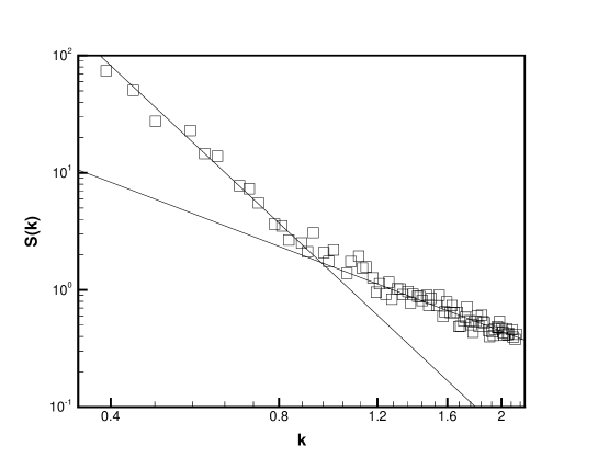
FIG. 12.: Structure factor as a function of $k$ at time $t=27$. The exponents of the power–law fits at small and large $k$ are 4.3 and 1.8 respectively. At small $k$ the structure factor is dominated by defects, while at large $k$ thermal fluctuations dominate.

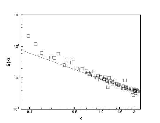
FIG. 13.: Structure factor as a function of $k$ at time $t=40$, near the end of the coarsening sequence. The crossover between the thermal fluctuation regime at large $k$ and the defect dominated regime at small $k$ occurs at smaller values of $k$ than at earlier times in the coarsening sequence (compare with Fig. 12). Due to the relatively small number of data points in the defect dominated regime, we have not attempted a power–law fit.

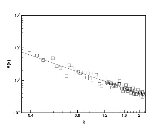
FIG. 14.: Structure factor as a function of $k$ at time $t=70$, after all of the defects have disappeared. The data is fit with an exponent of 1.7. With the coarsening process completed, only thermal fluctuations contribute to the structure factor.

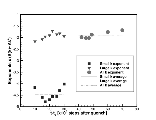
FIG. 15.: Values of the exponents used to fit the structure factor $S(k)$ at small and large values of $k$ as a function of time. Topological defects dominate the small $k$ behavior until the defects disappear around $t=40$, while thermal fluctuations dominate at large $k$. At later times thermal fluctuations are the only contribution to $S(k)$ for all $k$, and a single exponent fits the entire range of $k$. During the last stages of the coarsening sequence (between $t=30$ and $t=40$) we do not have sufficient numbers of data points to fit the small $k$ behavior because the crossover to the thermal fluctuation regime occurs at small $k$. However, the large $k$ behavior continues to be fit well with an exponent of approximately 2 (see Fig. 13). The solid and dashed lines indicate the average values of the exponents used to fit the large and small $k$ regimes of $S(k)$ during the coarsening sequence; the values are 1.9 and 4.5 in these regimes respectively. The dashed–dotted curve indicates the average exponent, 1.9, that fits all of the $k$ data after the defects have disappeared.

The crossover value of $k$ separating the defect dominated and thermal fluctuation dominated regimes is of the order of magnitude predicted by Eq. (9), namely, $k\sim(2\pi^{3}K\rho_{disc}/k_{B}T)^{1/3}\sim(24\pi^{4}\rho_{monop}/k_{B}T)^{1/4}$. This crossover value decreases with time, as can be seen by comparing Fig. 12 with the later time data of Fig. 13. The crossover value of $k$ in the latter figure is about half of the corresponding value in the former figure, consistent with the relative densities of defects at the two times.

As discussed in ref. [30] we would expect the crossover to the thermal fluctuation dominated regime to be accompanied by a breakdown of the dynamical scaling hypothesis because it assumes that thermal fluctuations play no role in the behavior of real–space or Fourier–space correlation functions. To test this expectation we used our data for $S(k,t)$ during the time range spanning the coarsening process to plot the scaling function $g$ defined in Eq. (8). This plot is shown in Fig. 16, where we clearly see the breakdown of scaling for $kL(t)$ greater than approximately 4 or 5, corresponding to values of $r/L(t)$ less than approximately one. Note that the numerical range of $g$ is much larger than the range of $f$, the corresponding scaling function for $C(r,t)$ (Eq. (7) and Fig. 11), so that the breakdown in scaling is easier to see in the structure factor data. The wider horizontal range for $kL(t)$ compared to $r/L(t)$ also makes the breakdown clearer.

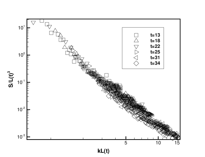
FIG. 16.: Plot of the dynamical scaling function $g=S(k,t)/(L(t))^{3}$ as a function of the scaling variable $kL(t)$, (see Eq. (8)). Note the clear breakdown of scaling for large values of $kL(t)$.

Note in our plots, $k\geq R^{-1}$, for nearly all values of the disclination loop radius $R$. Thus, in this regime we expect to see a power–law contribution to $S(k)$ from the twist dislination loops. With a simulation of a larger system it might be possible to study the regime $k\ll R^{-1}$ where the twist disclination loops are expected to make no contribution to $S(k)$, as discussed in Sec. II.

VI Conclusions

In conclusion, we have shown that the Gay-Berne potential is fruitful for studying the behavior of the wide variety of topological defects generated in a quench from the isotropic to the nematic phase. At least for the Gay-Berne parameters chosen here, twist disclination loops were the dominant defects, and we did not, aside from possibly one isolated line, observe dynamically generated wedge disclination loops. This result, if it is not an artifact of our relatively small system size, has important implications for the interpretation of scattering experiments on quenched nematics, following upon the ideas of Ref. [30]. As we discussed in Sec. II measurements of the structure factor show scaling with an exponent between 5 and 6. Twist disclination lines yield an exponent of 5, whereas monopoles (which are relatively few in number in experimental systems) and wedge disclination lines (which are not energetically favorable) yield 6. Thus, it remains an open question as to why the exponent observed is greater than 5 over some appreciable range of wavevector.

Our computed real–space correlation function exhibited good dynamical scaling over the limited range of distances available, though the structure factor appears to be provide a more sensitive test of scaling. In our structure factor data we could clearly see the breakdown of dynamical scaling and the crossover to the thermal fluctuation dominated behavior, in accord with the predictions of Zapotocky and Goldbart[30]. Clearly, simulations of even larger Gay-Berne systems would be of interest to further address the issues raised here.

REFERENCES

- [1] M. Bowick, L. Chandar, E. Schiff, and A. Srivastava, Science 263, 943 (1994).
- [2] I. Chuang, R. Durrer, N. Turok, and B. Yurke, Science 251, 1336 (1991).
- [3] M. Salomaa and G. Volovik, Rev. Mod. Phys. 59, 533 (1987).
- [4] A. Vilenkin and E. Shellard, Topological Defects and Cosmology (Cambridge University Press, Cambridge, 1994).
- [5] I. Chuang, B. Yurke, A. Pargellis, and N. Turok, Phys. Rev. E 47, 3343 (1993).
- [6] M. Mondello and N. Goldenfeld, Phys. Rev. A 45, 657 (1992).
- [7] R. Blundell and A. Bray, Phys. Rev. E 49, 4925 (1994).
- [8] H. Nishimori and T. Nukii, J. Phys. Soc. Jpn. 58, 563 (1989).
- [9] H. Toyoki, J. Phys. Soc. Jpn. 63, 4446 (1994).
- [10] M. Zapotocky, P. Goldbart, and N. Goldenfeld, Phys. Rev. E 51, 1216 (1995).
- [11] N. Goldenfeld, in Formation and Interactions of Topological Defects, Vol. 349 of B, NATO ASI, edited by A. Davis and R. Brandenberger (Plenum Press, N.Y., 1995), p. 103.
- [12] S. Bedford and A. Windle, Liq. Cryst. 15, 31 (1993).
- [13] C. Liu and M. Muthukumar, J. Chem. Phys. 106, 7822 (1997).
- [14] A. Kilian, Mol. Cryst. Liq. Cryst. 222, 57 (1992).
- [15] L. Pismen and B. Rubinstein, Phys. Rev. Lett. 69, 96 (1992).
- [16] S. Hudson and R. Larson, Phys. Rev. Lett. 70, 2916 (1993).
- [17] J. Gay and B. Berne, J. Chem. Phys. 74, 3316 (1981).
- [18] For a recent review see, J. Crain and A. V. Komolkin, Adv. Chem. Phys. 109, 39 (1999).
- [19] D. Lehmann, Die Lehre der flüssigen Kristallen und ihre Beziehung zu den Problemen der Biologie (Bergmann, Wiesbaden, 1917).
- [20] C. Oseen, Trans. Faraday Soc. 29, 883 (1933).
- [21] T. C. Lubensky, D. Pettey and H. Stark, Phys. Rev. E 57, 610 (1998).
- [22] M. Kléman, Points, Lines and Walls: In Liquid Crystals, Magnetic Systems and Various Ordered Media (Wiley, New York, 1983).
- [23] R. Meyer, Philos. Mag. 27, 405 (1973).
- [24] A. Pargellis, J. Mendez, M. Srinivasarao, and B. Yurke, Phys. Rev. E 53, R25 (1996).
- [25] C. Williams, P. Cladis, and M. Kleman, Mol. Cryst. Liq. Cryst. 21, 355 (1972).
- [26] A. Bray, Adv. Phys. 43, 357 (1994).
- [27] T. Kibble, J. Phys. A 9, 1387 (1976).
- [28] M. Hindmarsh, Phys. Rev. Lett. 75, 2502 (1995).
- [29] T. Nagaya, H. Hotta, H. Orihara, and Y. Ishibashi, J. Phys. Soc. Jpn. 61, 3511 (1992).
- [30] M. Zapotocky and P. Goldbart, cond-mat/9812235.
- [31] B. Yurke, A. Pargellis, and N. Turok, Mol. Cryst. Liq. Cryst. 222, 195 (1992).
- [32] R. E. Blundell. A. J. Bray, S. Puri and A. M. Somoza, Phys. Rev. E 47, 2261 (1993).
- [33] S. I. Anisimov and I. E. Dzyaloshinskii, Sov. Phys. JETP 36, 774 (1973).
- [34] S. Chandrasekhar and G. Ranganath, Adv. Phys. 35, 507 (1986).
- [35] A. P. Y. Wong, P. Wiltzius and B. Yurke, Phys. Rev. Lett. 69, 3583 (1992).
- [36] A. P. Y. Wong, P. Wiltzius, R. G. Larson and B. Yurke, Phys. Rev. E47, 2683 (1993).
- [37] G. Luckhurst, R. Stephens, and R. Phippen, Liq. Cryst. 8, 451 (1990).
- [38] R. Berardi, P. Emerson, and C. Zannoni, J. Chem. Soc. Faraday Trans. 89, 4069 (1993).
- [39] M. Allen and D. Tildesley, Computer Simulations of Liquids (Clarendon, Oxford, 1987).
- [40] M. R. Wilson, M. P. Allen, M. A. Warren, A. Sauron and W. Smith, J. Comput. Chem. 18, 478 (1997).
- [41] K. Strobl, Sussex University Report No. SUSX-96-012 (unpublished).
- [42] R. Ondris-Crawford, E. P. Boyko, B. G. Wagner,J. H. Erdmann, S. Zumer, J. W. Doane, J. Appl. Phys. 69, 6380 (1991).
- [43] J. Schellmann, in Polarized Spectroscopy of Ordered Systems, edited by B. Samori and E. Thulstrup (Kluwer, Dordrecht, 1988).
- [44] P. de Gennes and J. Prost, The Physics of Liquid Crystals (Clarendon Press, Oxford, 1993).
- [45] http://www.physics.brown.edu/Users/faculty/pelcovits/lc/coarsening.html
- [46] There is some possibility that this apparent wedge segment is in fact part of a twist line given our particular viewing perspective along the axis of the MD cell. See, Y. Bouligand,in Geometry and Topology of Defects in Liquid Crystals,edited by R. Balian, M. Kléman and J.-P. Poirier (North-Holland, Amsterdam, 1981) for a discussion of this possibility.
- [47] M. P. Allen, M. A. Warren and W. Smith, J. Chem. Phys. 105, 2850 (1996).