Heteroskedastic Lévy flights

Abstract

Truncated Lévy flights are random walks in which the arbitrarily large steps of a Lévy flight are eliminated. Since this makes the variance finite, the central limit theorem applies, and as time increases the probability distribution of the increments becomes Gaussian. Here, truncated Lévy flights with correlated fluctuations of the variance (heteroskedasticity) are considered. What makes these processes interesting is the fact that the crossover to the Gaussian regime may occur for times considerably larger than for uncorrelated (or no) variance fluctuations.

These processes may find direct application in the modeling of some economic time series.

I Introduction

The ubiquity of the Gaussian probability distribution function (PDF) in physics and statistics is a consequence of the central limit theorem (CLT) [2], which states that the PDF of the sum of $N$ independent, identically distributed (i.i.d.) stochastic variables whose variance is finite converges to the Gaussian PDF when $N\rightarrow\infty$.

If the hypothesis of finite variance is relaxed, a generalized CLT still exists [3, 4]: the PDF of the sum belongs to the family of Lévy stable distributions, defined by the characteristic function (Fourier-transform)

$$L(z)=\exp[{\rm i}mz-\gamma|z|^{\alpha}(1+{\rm i}\beta z/|z|\tan(\alpha\pi/2))]$$ (1)

with $0<\alpha\leq 2$. For $\alpha=2$ the Gaussian distribution is recovered, while for $\alpha<2$ the PDF possesses power-law tails $L(x)\sim Cx^{-(1+\alpha)}$ which make the variance infinite. In this article, only symmetrically distributed stochastic variables are considered, for which $m=\beta=0$.

A Lévy flight [3, 4, 5] (LF) is a random walk in which the step length is chosen from the PDF of Eq. (1). Since Lévy distributions are stable under convolution, the LF process is self-similar, i.e. the same Lévy distribution describes increments over different time scales, provided the increments are appropriately rescaled.

Lévy flights appear in various physical problems [5, 6], in particular diffusion, fluid dynamics, and polymers. However, because of their infinite variance and lack of a characteristic scale, Lévy PDFs overestimate the probability of extreme events when used to model real physical systems, for which an unavoidable cutoff is always present [7]. The most direct way to make the variance finite is by means of truncated Lévy (TL) PDFs [7]. The TL PDF is close to a Lévy PDF for small argument, but it contains a sharp [7] or exponential [8] cutoff in the tails. A truncated Lévy flight (TLF) is a random walk in which the step length is chosen from a TL PDF.

The TL PDF belongs to the basin of attraction of the Gaussian PDF: for large $N$ the sum of $N$ i.i.d. TL variables is Gaussian-distributed. For small $N$ the central part of the PDF of the sum has a Lévy shape, but the variance and higher moments are finite. For symmetric TL PDFs the deviation from a Gaussian may be quantified by the value of the normalized fourth cumulant (kurtosis, $\kappa$) [2]. This is zero for a Gaussian, and positive for a TL PDF. The crossover to the Gaussian regime is given by $N\gg N_{0}\propto l^{\alpha}$ with $l$ the cutoff length. Under this condition, $\kappa$ becomes very small (see Eq. (20)).

In this article, the TLF stochastic process is generalized to include a special form of nonlinear dependence of the increments called heteroskedasticity. One can build processes with dependent increments such that the central part of the PDF of the sum still approximately behaves as in a Lévy flight. What is remarkable and makes these processes interesting is the fact that the crossover to the Gaussian PDF may be pushed to values of $N$ which are larger by some order of magnitudes than if the increments were independent.

II Lévy PDF in economic time series

Besides being interesting per se, these processes are of direct of relevance to one of the most noteworthy applications of LF outside physics, i.e. to the modeling of some financial time series [9]. From a physicist’s perspective, the market is a very good example of a complex system [10, 11, 12] in which the mutual interaction and competition among a great number of agents (traders or speculators) with continually adapting strategies, together with the influence of unpredictable exogenous factors, usually produces an intricate out-of-equilibrium dynamics.

In the classical equilibrium theory of economy it is assumed that “equilibrium” values for the prices exist, satisfying an aggregate, overall consistency condition (recalling the so called Nash equilibria solutions of game theory [13]). However, the complex dynamics of market prices does not seem to fit this classical picture. In particular, trading volume and price volatility are much higher than expected from the classical theory [14]. From time to time, the market may display strong movements (crashes or boosts) which cannot always be understood in terms of rational reactions to incoming new information [15]. Instead, some of their features recall the physical concept of self-organized criticality [16].

At last, trading volumes and variances of price increments change over time [17], and may persist as low or high for long periods. The existence of such correlated variance fluctuations (heteroskedasticity) is difficult to understand in the framework of classical equilibrium theory, and few economic models can explain it (see e.g. Ref. [18] where an equilibrium model capable to mimic volatility fluctuations of interest rates is developed).

A fundamental source of this complex dynamics may be found in the inductive, subjective and adaptive nature of the process leading agents to formulate the expectations which drive their actions [10, 19, 20, 21, 22, 23], an aspect whose fundamental features can be captured by more or less elaborated game or artificial-life models [10, 21, 24, 25, 26, 27, 28, 29].

Aside the ”microscopic” origin of the complexity of financial markets, another aspect of the problem is the phenomenological (”macroscopic”) characterization of this complexity, in particular the study of the properties of economic time series. Given the low level of determinism of these series, the most fruitful description is in terms of stochastic processes. Martingale processes [2] are the signature of market efficiency. In particular, random walk or Brownian-motion models have been used for a long time to model the increments of asset prices [30]. This might be understood by the central limit theorem if price changes resulted from the sum of many independent random contributions, which would seem a reasonable assumption. Indeed, empirical studies of financial time series have revealed gaussian behavior for long time scales, typically of the order of several days. However, it has been shown [9] that for short time scales the central part of the PDF is not Gaussian. It is well described by a Lévy distribution, and therefore suggests an underlying LF rather than random-walk model.

Non-gaussian scaling has been found in many economical or financial indeces [9, 32, 33, 34, 35, 36, 37, 38]. In financial time series, scale invariance can be characterized (i.e. the value of the self-similarity exponent $\alpha$ in Eq. (1) can be extracted) either by comparing the full PDF of price increments over different time scales, or by studying the time-scale dependence of some selected properties of the PDF. For example, the probability of return

$$P_{N}(x=0)=\frac{1}{\pi}\int_{0}^{\infty}(L(z))^{N},$$ (2)

which depends on the time scale $N$ as $N^{-1/\alpha}$, was used to extract the value $\alpha\sim 1.40$ in the high-frequency (one-minute) variations of the Standard & Poor’s 500 (S&P500) index [9, 31]. An alternative quantity which may be used is the so-called Hurst exponent (see, e.g., Ref. [37]).

As with other applications of LF, while Lévy distributions describe well the central part of the PDF for short times, the power-law tails of these distributions are much fatter than observed. In particular, the observed variance is finite. All the previous remarks suggest the TLF as the best candidate to model these series [37, 39].

Two aspects, however, remain unexplained : one is the fact that the crossover to the Gaussian regime occurs at much larger times than expected from the TLF model (and from any model with i.i.d. increments as well). For example, the one-minute PDF $P_{1}$ of the S&P500 index increments has kurtosis $\kappa_{1}=43$ [9, 39]. If the PDF at time $N$, $P_{N}$, were $P_{1}$ convoluted $N$ times with itself (with kurtosis $\kappa_{N}=\kappa_{1}/N$), Gaussian behavior would be expected for $N\gg\kappa_{1}$ (see Fig. 1). However, the central part of $P_{N}$ displays Lévy behavior up to at least $N=1000$ [9].

The second aspect not accounted for is heteroskedasticity: even if linear correlations are almost zero, there are correlations of the squared increments, i.e. the increments at different times are uncorrelated yet not independent random variables. Put another way, one cannot factorize the joint probability density of the increments at different times into the product of reduced densities.

The model proposed in the following can account at the same time for both these aspects.

III Models for heteroskedasticity

A Gaussian-type models

Many efforts have been devoted in the past two decades to the study of time-varying variance, and various models have been put forward by econometricians. Roughly, two great classes of models exist : Auto-Regressive-Conditional-Variance (ARCH) type models and Stochastic-Variance (SV) type models.

Models of both classes are usually set up in a Gaussian framework: if time is discretized with an elementary time step $\tau$, the increments at the $k$-th time-step (i.e. at $t=k\tau$) are assumed to be random variables of the form

$$x_{k}=\mu_{k}+\sqrt{v_{k}}\epsilon_{k}.$$ (3)

Here $\mu_{k}$ is the time-varying mean of the stochastic process ($\mu_{k}$ is very small, and can safely be set to zero, for the short time scales considered here), $v_{k}$ is a random variable representing the time-varying variance of the process, and the $\epsilon_{k}$ are independent Gaussian random variables with zero mean and unit variance, independent of $v_{k}$.

ARCH and SV models differ in the way the $\sigma_{k}$ process is specified : in ARCH-type models [40, 41] the variance at time-step $k$ is a deterministic function of the past squared increments and variances, while in SV-type models [42] the variance is not completely determined by the past data, since it contains a random contribution. With suitable choices of their parameters, both type of models can account for the heteroskedasticity and positive kustosis (leptokurtosis) of the PDF of financial series, although usually they fail to capture all aspects of the data [43]. In particular, it has been shown by numerical simulations in Ref. [39] that the simplest ARCH-type models do not yield the Lévy-type scaling of the PDF described above, since already at short times the value of the scaling exponent is close to the gaussian one.

B General models

Let us assume the $x_{k}$ to be zero-mean random variables with variance $v_{k}$, with a symmetric PDF $P_{1}^{v_{k}}(x_{k})$ depending on the parameter $v_{k}$ in an as yet unspecified way. The parameter $v$ fluctuates in time following a stationary process. Let $p_{N}(v_{1},\cdot\cdot,v_{N})$ be the joint PDF of the variances at the different times, and let us assume the joint PDF of increments and variances

$$P_{N}(x_{1},\cdot\cdot,x_{N};v_{1},\cdot\cdot,v_{N})=p_{N}(v_{1},\cdot\cdot,v_{N})\prod_{i}P_{1}^{v_{i}}(x_{i}),$$ (4)

i.e. the increments conditional to a certain set of variances $v_{1},\cdot\cdot,v_{N}$ are independent variables. However, $P_{N}(x_{1},\cdot\cdot,x_{N};v_{1},\cdot\cdot,v_{N})$ is not directly observable. The object of measurement is the unconditional PDF

$$P^{unc}_{N}(x_{1},\cdot\cdot,x_{N})=\int dv_{1}\cdot\cdot dv_{N}P_{N}(x_{1},\cdot\cdot,x_{N};v_{1},\cdot\cdot,v_{N}),$$ (5)

which is only factorized if $p_{N}(v_{1},\cdot\cdot,v_{N})$ is.

A special case of process with PDF given by Eq. (4) is

$$x_{k}=\sqrt{v_{k}}\xi_{k},$$ (6)

where the $\xi_{k}$ are independent random variables with zero mean and unit variance, independent of $v_{k}$, and with PDF $P_{0}(\xi)$. In this case,

$$P_{1}^{v}(x)=\frac{1}{\sqrt{v}}P_{0}(\frac{x}{\sqrt{v}}).$$ (7)

For this special process the PDF is assumed to change with time only through a time-varying scale factor. The process reduces to that of Eq. (3) if $P_{0}$ is Gaussian, however $P_{0}$ does not necessarily need to be gaussian. For example, in Ref. [44] ARCH-type processes with a $t$-Student $P_{0}$ are used.

The characteristic function of $P_{1}^{v}(x)$ is

$$P_{1}^{v}(z) = \int dx\exp(izx)P_{1}^{v}(x)$$ (8)

$$\rightarrow P_{0}(\sqrt{v}z).$$ (9)

Here and in the following $\rightarrow$ indicates the result for the particular case of a scale-factor-type process, Eq. (6). $P_{0}(z)$ is the characteristic function of $P_{0}(x)$.

$P_{1}^{v}(z)$ can be used [2] to calculate moments and cumulants of $P_{1}^{v}(x)$ of any order $n$,

$$m_{n}^{v}(1) = (-{\rm i})^{n}\frac{{\rm d}^{n}}{{\rm d}z^{n}}P_{1}^{v}(z)|_{z=0}\rightarrow v^{\frac{n}{2}}m_{n}^{0}$$ (10)

$$c_{n}^{v}(1) = (-{\rm i})^{n}\frac{{\rm d}^{n}}{{\rm d}z^{n}}\log P_{1}^{v}(z)|_{z=0}\rightarrow v^{\frac{n}{2}}c_{n}^{0},$$ (11)

$m_{n}^{0}$ and $c_{n}^{0}$ being moments and cumulants of $P_{0}$. The assumed symmetry of $P_{1}^{v}(x)$ implies that all its odd-order moments vanish. The variance $m_{2}^{v}(1)=c_{2}^{v}(1)=v$. The normalized cumulants are

$$\eta_{n}^{v}(1)=\frac{c_{n}^{v}(1)}{v^{\frac{n}{2}}}\rightarrow c_{n}^{0}.$$ (12)

The kurtosis $\kappa^{v}(1)=\eta_{4}^{v}(1)$ is zero for the process of Eq. (3).

1 Unconditional PDF for N=1

.

For the Gaussian-type processes of Eq. (3), it is easy to extract $p_{1}(v)$ from a given measured $P_{1}^{unc}(x)$. Using Eqs. (4), (5) and (9) its characteristic function $P_{1}^{unc}(z)$ is found to be

$$P_{1}^{unc}(z)=\int{\rm d}vp_{1}(v)\exp(-\frac{v}{2}z^{2}).$$ (13)

Since $p_{1}(v)=0$ for $v<0$ (the variance has to be positive), Eq. (13) is a Laplace transform. Setting $z^{2}/2=s$, $P_{1}^{unc}(\sqrt{2s})={\cal L}(p_{1}(v))$. Thus, the PDF of the variance $p_{1}(v)$ giving an observed $P_{1}^{unc}(z)$ is the inverse Laplace transform $p_{1}(v)={\cal L}^{-1}(P_{1}^{unc}(\sqrt{2s}))$. If $P_{1}^{unc}(z)$ is a symmetric Lévy PDF with index $\alpha$, it follows that $p_{1}(v)$ is itself a Lévy PDF Eq. (1) of index $\alpha/2$ and asymmetry $\beta=1$, $m=0$ [4]. This latter has an essential singularity at $x=0$. If $P_{1}^{unc}(z)$ is a symmetric TL PDF, the singular behavior close to $x=0$ remains, but the decrease of $p_{1}(v)$ for $v\rightarrow\infty$ changes from algebraic to exponential.

For a general process such Laplace-transform relationship is lost. By differentiating $P_{1}^{unc}(z)$ at $z=0$, moments $m_{n}^{unc}(1)$ of $P_{1}^{unc}(x)$ of any order $n$ can be expressed in terms of moments of $P_{1}^{v}(x)$ :

$$m_{n}^{unc}(1)=(-{\rm i})^{n}\frac{{\rm d}^{n}}{{\rm d}z^{n}}P_{1}^{unc}(z)|_{z=0}=\langle m_{n}^{v}(1)\rangle_{v},$$ (14)

where $\langle f(v)\rangle_{v}=\int{\rm d}vp_{1}(v)f(v)$ and $m_{n}^{v}(1)$ is the $n$-th-order moment of $P_{1}^{v}(x)$, Eq. (10). The kurtosis of $P_{1}^{unc}(x)$ is

$$\kappa^{unc}(1)=\frac{m_{4}^{unc}(1)}{(m_{2}^{unc}(1))^{2}}-3\rightarrow\frac{\langle v^{2}\rangle_{v}}{\langle v\rangle_{v}^{2}}(\kappa_{0}+3)-3,$$ (15)

where $\kappa_{0}$ is the kurtosis of $P_{0}$. As is well-known, a fluctuating variance (for which $\langle v^{2}\rangle_{v}\neq\langle v\rangle_{v}^{2}$) can produce a non-Gaussian PDF ($\kappa^{unc}(1)\neq 0$) even when $P_{0}$ is Gaussian ($\kappa_{0}=0$). Thus, a given measured $P_{1}^{unc}(x)$ may be consistent with many different choices of the couple ($P_{1}^{v}(x)$ , $p_{1}(v)$), which explains the existence of many econometric models. For example, the observed leptokurtic character of $P_{1}^{unc}(x)$ may arise either from a leptokurtic $P_{0}$ or from fluctuations of the variance or from both effects.

2 Unconditional PDF for N $>$ 1

At time $N>1$ the characteristic function of the unconditional PDF of the sum, $P_{N}^{unc}(x)$, $x=\sum_{i=1}^{N}x_{i}$, is found from Eq. (4),

$$P_{N}^{unc}(z)=\int{\rm d}v_{1}\cdot\cdot{\rm d}v_{N}p_{N}(v_{1},\cdot\cdot,v_{N})\prod_{i=1}^{N}P_{1}^{v_{i}}(z).$$ (16)

For independent variance fluctuations, $p_{N}(v_{1},\cdot\cdot,v_{N})=\prod_{i}p_{1}(v_{i})$, and $P_{N}^{unc}(x)$ is simply given by $P_{1}^{unc}(x)$ convoluted $N$ times with itself. In this case cumulants, including the variance, scale as $N$. The kurtosis decreases as $\kappa^{unc}(N)=N^{-1}\kappa^{unc}(1)$.

If fluctuations of the variance are correlated, by differentiating Eq. (16) at $z=0$, moments of $P_{N}^{unc}(x)$ of any order $n$ may be expressed in terms of averages of products of moments of $P_{1}^{v}(x)$ taken at different times, the average being made over $p_{N}(v_{1},\cdot\cdot,v_{N})$. The variance scales as $m_{2}^{unc}(N)=Nm_{2}^{unc}(1)$, just as for uncorrelated (or no) variance fluctuations. The kurtosis depends on linear correlations of the variances[45] :

$$\kappa^{unc}(N)=\kappa^{unc}(1)/N+{\tilde{\kappa}}^{unc}(N)$$ (17)

$${\tilde{\kappa}}^{unc}(N)=6(2+\kappa^{unc}(1))\sum_{d=1}^{N}(1/N-d/N^{2})g(d)$$ (18)

$$g(d)=\frac{\langle v_{1}v_{1+d}\rangle_{v}-\langle v\rangle_{v}^{2}}{\langle m_{4}^{v}(1)\rangle_{v}-\langle v\rangle_{v}^{2}}=\frac{\langle\langle x^{2}_{1}x^{2}_{1+d}\rangle\rangle-\langle\langle x^{2}\rangle\rangle^{2}}{\langle\langle x^{4}\rangle\rangle-\langle\langle x^{2}\rangle\rangle^{2}},$$ (19)

where $\langle..\rangle_{v}$ is an average over variance fluctuations, and $\langle\langle..\rangle\rangle$ is an average over fluctuations of the $x_{i}$ and the variances. The normalized two-times autocorrelation of the squared increments, $g$, determines the degree of persistence of variance fluctuations. The simplest models of the type of Eq. (3) (such as those considered in Ref. [39]) have a positive $g(d)\sim K\exp(-d/d_{0})$. In Ref. [36] $g(d)\sim g_{0}d^{-0.37}$ is found from the 5-minute increments of the S&P500 index. In any case, in presence of positive variance correlations, $\kappa^{unc}(N)$ may decrease with $N$ much more slowly than if $g(d)=0$. Thus, roughly speaking, the slowing down of the decrease of $\kappa^{unc}(N)$ pushes the onset of a Gaussian regime ($\kappa^{unc}(N)\rightarrow 0$) to much larger values of $N$ than expected from independent (or no) variance fluctuations. The problem is that for most models, and in particular those of the type of Eq. (3), these heteroskedastic contributions to $P_{N}^{unc}(x)$ may be inconsistent with Lévy behavior close to $x=0$.

To make the variance autocorrelation $g$ explicit in $P_{N}^{unc}(z)$, it is convenient to characterize the stochastic process followed by the variances by its multivariate characteristic function $p_{N}(k_{1},\cdot\cdot,k_{N})$. For independent $v_{k}$, $p_{N}(k_{1},\cdot\cdot,k_{N})=\prod_{i}p_{1}(k_{i})$, $p_{1}(k)$ being the Fourier transform of $p_{1}(v)$. When correlations are present, $p_{N}(k_{1},\cdot\cdot,k_{N})$ may be expressed as

$$p_{N}(k_{1},\cdot\cdot, k_{N} )=\exp(-A\sum_{i<j}g(i-j)k_{i}k_{j}+S)\prod_{i}p_{1}(k_{i})$$ (20)

$$= \prod_{i}p_{1}(k_{i})(1-A\sum_{i<j}g(i-j)k_{i}k_{j}+\cdot\cdot).$$ (21)

Here $A=\langle m_{4}^{v}(1)\rangle_{v}-\langle v\rangle_{v}^{2}$, and $S=o((|k_{1}|+\cdot\cdot+|k_{N}|)^{2})$ contains contributions from mixed cumulants of $p_{N}(v_{1},\cdot\cdot,v_{N})$ of order higher than two [46], e.g. terms of type $k_{i}k_{j}k_{l}$ or $k_{i}k_{j}k_{l}k_{s}$ with the time indices $i$, $j$, $l$, $s$ not all equal. These describe correlations of the variances of higher order than those described by $g$. The approximation of putting $S=0$ corresponds to make a Gaussian-like decoupling of these high-order correlations into products of linear two-times ($g(d)$) and equal-time correlations (e.g., $\langle v_{1}^{3}v_{2}\rangle=3g(1)\langle v^{2}\rangle+\langle v\rangle\langle v^{3}\rangle$).

Let us consider, for example, models of the type of Eq. (3), which are the most commonly used. For these models it has been shown (Eq. (13)) that it is possible to choose $p_{1}(v)$ such that $P_{1}^{unc}(x)$ is a TL PDF. By using Eq. (18), $g(d)$ may be made explicit in $P_{N}^{unc}(z)$ , Eq. (16). By a few simple manipulations, it is possible to sum up all the contributions of $g$ to $P_{1}^{unc}(z)$ to obtain

$$P_{N}^{unc}(z)\!=\!P_{1}^{unc}(z)^{N}\!\exp(\frac{Az^{4}}{4}\!\sum_{i<j}g(i-j)\!+\!{\cal O}(z^{6}))$$ (22)

It is peculiar to the processes of Eq. (3) that the contributions ${\cal O}(z^{6})$ do not depend on $g$, but only on higher-order correlations ($S$ in Eq. (18)). More specifically, mixed cumulants of order $p$ in Eq. (18) give terms ${\cal O}(z^{2p})$ in the exponent of Eq. (19). To produce a Lévy scaling of $P_{N}^{unc}(x)$ for small $x$, $P_{N}^{unc}(z)$ has to behave as $[P_{1}^{unc}(z)]^{N}\sim\exp(-N\gamma|z|^{\alpha})$ for large $z$. Then, constraints should be put on variance correlations of any order to ensure that as $z\rightarrow\infty$ the exponent in Eq. (19) does not diverge more strongly than $z^{\alpha}$. It is also possible that for large $z$ the contributions of variance fluctuations to $P_{N}^{unc}(z)$ be not determined by its small $z$ behavior, i.e. by its moments [2]. In turn, this may happen if $p_{N}(v_{1},\cdot\cdot,v_{N})$ itself is not uniquely determined by its moments, i.e. $p_{N}(k_{1},\cdot\cdot,k_{N})$ has singularities. Anyway, such non-analytic contributions would not yield a Lévy scaling in general.

IV Truncated Lévy flights with heteroskedasticity

It has been shown above that if the elementary PDF $P_{1}^{v}(x)$ is Gaussian, Lévy behavior of $P_{N}^{unc}(x)$ may be obtained only by making ad hoc assumptions about $p_{1}(v)$ and the multivariate structure of variance fluctuations, which looks somewhat artificial. It is simpler and more intuitive to assume, instead, that for some $v$, $P_{1}^{v}(x)$ itself is equal or close to a TL PDF. There are many possible ways to choose how the parameter $v$ should enter. If a TL PDF with exponential cutoff at $l\sim\lambda^{-1}$[8] is used for $P_{1}^{v}$, its variance and kurtosis are, respectively,

$$v=\frac{\gamma\alpha(\alpha-1)\lambda^{\alpha-2}}{|\cos(\pi\alpha/2)|}\hskip 5.69046pt{\rm,}\hskip 5.69046pt\kappa=\frac{(\alpha-3)(\alpha-2)}{\lambda^{2}v}.$$ (23)

If the scaling exponent $\alpha$ is fixed, a time-varying $v$ may occur either through variations of $\gamma$ (these reflect variations of trading volumes in economic applications), or variations of the cutoff $\lambda$ or of both.

Although the central part of a superposition of TL PDFs with varying $\gamma$ does not have an exact Lévy behavior, this behavior still exists approximately for many choices of $p_{1}(v)$, i.e. one can find a Lévy PDF with the same $\alpha$ and an effective $\gamma$ which describes approximately the central part of the superposition. For example, if $v$ or $\gamma$ have a lognormal PDF (given that $v$, $\gamma>0$ this is a simple possible candidate PDF), the central part of the superposition is dominated by the $\gamma$ corresponding to the peak of the lognormal (non-Gaussian region, high kurtosis), while the tail for $\gamma\rightarrow\infty$ (quasi-Gaussian region, small kurtosis) mostly affects the tails of the superposition. In general, the smaller values of $\gamma$ determine the small $x$ behavior of $P_{1}^{unc}(x)$. On the other hand, the central part of a superposition of TL PDFs with varying cutoff $\lambda$ keeps an almost exact Lévy behavior, since $\lambda$ only affects the tails of the PDF.

In the following we focus on some qualitative features of TLF with correlated fluctuations of the variance. We study the simplest conceivable non trivial model, which nevertheless contains the relevant features of this type of processes, and has the advantage that an accurate numerical evaluation of $P_{N}^{unc}(x)$ can be made without approximations. The variance is assumed to fluctuate between two possible values only, $v_{a}$ and $v_{b}$, $v_{a}<v_{b}$. Thus, $p_{1}(v)=p_{a}\delta(v-v_{a})+(1-p_{a})\delta(v-v_{b})$. If $p_{a}\gg 0.5$ one may view $p_{1}(v)$ as a stylized lognormal PDF, with $v_{a}$ representing the position of the maximum and $v_{b}$ representing the tail of the lognormal. For $P_{1}^{v_{a}}$ we use a TL PDF with high kurtosis (strongly non-Gaussian behavior). $P_{1}^{v_{b}}$ should represent a TL PDF with small kurtosis (quasi-Gaussian behavior). To simplify the model as much as possible, and minimize the number of parameters, $P_{1}^{v_{b}}$ is assumed to be Gaussian with variance $v_{b}$. Thus, $P_{1}^{unc}=p_{a}P_{1}^{v_{a}}+(1-p_{a})P_{1}^{v_{b}}$.

For the stochastic process followed by the variances, the simplest choice is a Markov chain [2]. Thus, $p_{N}(v_{1},\cdot\cdot,v_{N})$ is determined by assigning the probability $p_{a}$ at time $N=1$, and the transition probabilities $p_{aa}$ and $p_{bb}$, i.e. the probability that if $v=v_{a}$ (or $v=v_{b}$) at any time $N$, then $v=v_{a}$ (or $v=v_{b}$) at time $N+1$. If the condition that the Markov chain be stationary is imposed, two free parameters, i.e. $p_{a}$, and $p_{bb}$, are left for the chain. These are to be added to the 3 parameters ($\alpha$, $\gamma$, $\lambda$ or, using Eq. (20), $\alpha$, $v_{a}$, $\kappa_{a}$) which fix $P_{1}^{v_{a}}$ and the single parameter ($v_{b}$) which fixes $P_{1}^{v_{b}}$. Note that for this model $g(d)$, Eq. (17), decays exponentially with $d$.

For the purpose of illustration, we try to apply this stylized model to the S&P500 data of Refs. [9, 31]. Four parameters are fixed by the values $\alpha=1.4$, $m_{2}^{unc}(1)\sim 0.016$ [47], $\kappa^{unc}(1)=43$, $P_{1}^{unc}(x=0)\sim 15$ measured for the 1-min. increments of the S&P500 index for the period 1984-1989. A fifth parameter is fixed by the decay rate $d_{0}$ of $g(d)$. Although by the Markov chain model it is not possible to directly reproduce the measured algebraically decaying $g(d)$, we do not expect this to affect the results qualitatively as long as the kurtosis is qualitatively well mimicked. Thus $d_{0}$ is fixed ($d_{0}\sim 126$ minutes), roughly, by demanding $\kappa^{unc}(N)$, Eq. (17) (see Fig. 1), to be be equal to unity at the same value $N\sim 3700$ which is found from Eq. (17) if one uses for $g(d)$ the same expression $g(d)\sim 0.08d^{-0.37}$ found in Ref. [36] for the 5-min increments of the S&P500 index future for the period 1991-1995. Since the time window and the time step of Ref. [36] are not the same of Refs. [9, 31], the value of $d_{0}$ is only indicative.

One parameter ($p_{a}$) remains free, and is fixed at 0.9 (any value close to one gives similar results).

As it may be seen in the inset of Fig. 1, the central part of $P_{1}^{unc}(z)$ is close to a Lévy PDF. $P_{N}^{unc}(z)$ is evaluated up to $N=10000$ by performing $4\cdot 10^{7}$ simulations of the Markov chain, enough to ensure full convergence of the results. These simulations yield a numerical estimation of the multivariate probability distribution of the variances $p_{N}(v_{1},\cdot\cdot,v_{N})$, by which $P_{N}^{unc}(z)$ is calculated through Eq. (16). $P_{N}^{unc}(x)$ is then calculated by a numerical Fourier transform of $P_{N}^{unc}(z)$.

The probability of return $P_{N}^{unc}(x=0)$ is plotted in Fig. 1. For comparison, $P_{N}^{unc}(x=0)$ is plotted for uncorrelated variance fluctuations (in this case $P_{N}^{unc}(z)=(p_{a}P_{1}^{v_{a}}(z)+(1-p_{a})P_{1}^{v_{b}}(z))^{N}$), and for a TLF with i.i.d. increments and again $\alpha=1.4$, $m_{2}(1)\sim 0.016$, $\kappa(1)=43$. As expected, for the two latter models, the onset of a Gaussian regime ($P_{N}^{unc}(x=0)\sim N^{-0.5}$) occurs as soon as $N\gg\kappa^{unc}(1)$. This would not be in agreement with observations, since Lévy scaling, $P_{N}^{unc}(x=0)\sim N^{-1/\alpha}$, is observed up to at least $N=1000$. Instead, for the heteroskedastic model the kurtosis decreases much more slowly (see Fig. 1) and the Gaussian regime occurs for much larger values of $N$. An approximate Lévy scaling persists up to $N\sim 2000$. In the inset it is shown that such approximate scaling extends to finite values of $x$ as well, $P_{N}^{unc}(x)\sim P_{1}^{unc}(xN^{-1/\alpha})N^{-1/\alpha}$ [9]. Gaussian scaling is estimated to occur only for $N\gtrsim 30000$.

V Conclusions

In conclusion, TLF with correlated fluctuations of the variance (heteroskedasticity) have been considered. These processes may be of relevance to the modeling of some financial time series. An explicit numerical calculation has been made by using for the stochastic process followed by the variances the simplest conceivable model, i.e. a Markov chain. Parameters suitable to model the behavior of the S&P500 stock index have been chosen for illustration.

The central part of the PDF of the increments during one time step, $P_{1}^{unc}(x)$, is close to a Lévy PDF. What makes these stochastic processes interesting is the fact that Lévy scaling of the PDF may persist for times order of magnitudes larger than for uncorrelated (or no) variance fluctuations.

It has also been shown that, using the Gaussian-type models of Eq. (3), a Lévy scaling of the PDF may be obtained only when quite ad hoc assumptions about the multivariate structure of variance fluctuations are made.

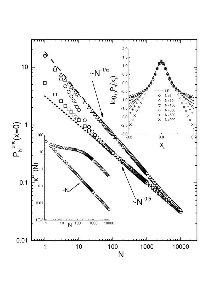
FIG. 1.: Probability of return vs time $N$. Triangles : truncated Lévy flight with Markov-chain heteroskedasticity (HLF) and parameters $p_{a}=0.9$, $p_{bb}=0.9929$, $\alpha=1.4$, $v_{a}=0.00393$, $\kappa_{a}=500$, $v_{b}=0.1246$, (see text). $g(N)\sim\exp(-N/126)$. Circles : i.i.d. variance fluctuations, $g(N>1)=0$. Squares : TLF with $v=0.016$, $\kappa=43$. Lower inset : kurtosis vs time $N$ for the HLF (triangles) and for the two other non heteroskedastic processes (circles). Upper inset : scaled PDF, $P_{s}(X_{s})=N^{1/\alpha}P_{N}^{unc}(X_{s})$, $X_{s}=xN^{1/\alpha}$ for the HLF with various values of $N$ compared with a Lévy PDF with $\alpha=1.4$ and $\gamma=0.0037$.

REFERENCES

- [1] On leave at Oxford Physics, Clarendon Laboratory, Parks Road, Oxford OX1 3PU, UK. E-mail : paolo.santini@ipt.unil.ch
- [2] W. Feller, An introduction to probability theory and its applications (Wiley, NY 1971).
- [3] P. Lévy, Théorie de l’addition des variables aléatoires (Gauthier-Villars, Paris, 1937).
- [4] B. V. Gnedenko and A. N. Kolmogorov, Limit distributions for sums of independent random variables (Addison-Wasley, Reading, MA, 1954).
- [5] J.-P. Bouchaud and A. Georges, Phys. Rep. 195 (1990) 127.
- [6] Lévy Flights and Related Phenomena in Physics M. F. Shlesinger, U. Frisch and G. Zaslavsky eds. (Springer Verlag, Berlin, 1995).
- [7] R. N. Mantegna and H. E. Stanley, Phys. Rev. Lett. 73 (1994) 2946.
- [8] I. Koponen, Phys. Rev. E 52 (1995) 1197.
- [9] R. N. Mantegna and H. E. Stanley, Nature (London) 376 (1995) 46.
- [10] W. B. Arthur, Complexity 1 (1995) 20.
- [11] The economy as an evolving complex system, P. W. Anderson, K. J. Arrow and D. Pines eds., Addison-Wesley, Redwood City (1988).
- [12] The economy as an evolving complex system II, W. B. Arthur, S. Durlauf and D. Lane eds., Addison-Wesley, Reading (1997).
- [13] H. W. Kuhn (Editor), Classics in Game Theory (Frontiers of Economic Research), Princeton Univ. Press (1997).
- [14] R. J. Shiller, in Advances in behavioral finance, R. H. Thaler editor (1993) 107.
- [15] D. M. Cutler, J. M. Poterba and L. H. Summers, in Advances in behavioral finance, R. H. Thaler editor (1993) 133.
- [16] D. Sornette, A. Johansen and J.-P. Bouchaud, J. Phys. I (France) 6 (1996) 167. D. Sornette and A. Johansen, Physica A 245 (1997) 411. D. Sornette and A. Johansen, Physica A 261 (1998) 581. A. Johansen and D. Sornette, Eur. Phys. J. B 1 (1998) 141.
- [17] P. K. Clark, Econometrica 41 (1973) 135.
- [18] W. J. den Haan and S. A. Spear, J. of Monetary Economics 41 (1998) 431.
- [19] G. Soros, The Alchemy of finance, J. Wiley and Sons, NY (1987).
- [20] J. H. Holland, The global economy as an adaptive process, in [11], p. 117.
- [21] W. B. Arthur, Amer. Econ. Review 84 (1994) 406.
- [22] S. Morris, Econometrica 62 (1994) 1327.
- [23] U. A. Müller, M. M. Dacarogna, R. D. Davé, R. Olsen, O. V. Pictet and J. E. von Weizsäcker, J. of Empirical Finance 4 (1997) 213.
- [24] L. Blume and D. Easley, J. of Economic Theory 58 (1992) 9.
- [25] W. B. Arthur, J. H. Holland, B. LeBaron, R. Palmer and P. Tayler, Physica D 75 (1994) 264.
- [26] G. Caldarelli, M. Marsili and Y.-C. Zhang, Europhys. Lett. 41 (1997) 479.
- [27] B. Chopard and R. Chatagny, Models of artificial foreign exchange markets, in Scale invariance and beyond, B. Dubrulle, F. Graner and D. Sornette eds., Springer-Verlag, Berlin (1997).
- [28] B. LeBaron, W. B. Arthur, R. Palmer, to appear on J. of Economic Dynamics and Control.
- [29] T. Lux and M. Marchesi, Nature (London) 397 (1999) 498.
- [30] Actually, it is usually assumed that the prices move according to a geometric brownian motion, which means that their logarithm follows a brownian motion (see, e.g., J. C. Hull, Options, futures and other derivative securities, Prentice Hall London (1997)).This is because the relevant variables are not absolute price increments, but returns, i.e. relative price increments. However, for the short time scales considered in this paper, the difference between the two descriptions is small [9, 37].
- [31] R. N. Mantegna and H. E. Stanley, Physica A 239 (1997) 255.
- [32] B. Mandelbrot, J. of Business 34 (1963) 392.
- [33] R. N. Mantegna, Physica A 179 (1991) 232.
- [34] R. N. Mantegna and H. E. Stanley, J. Stat. Phys. 89 (1997) 469.
- [35] D. Zajdenweber, Scale invariance in economics and finance, in Scale invariance and beyond, B. Dubrulle, F. Graner and D. Sornette Eds., Springer-Verlag, Berlin (1997).
- [36] R. Cont, M. Potters and J.-P. Bouchaud, Scaling in stock market data : stable laws and beyond, in Scale invariance and beyond, B. Dubrulle, F. Graner and D. Sornette Eds., Springer-Verlag, Berlin (1997).
- [37] J.-P. Bouchaud and M. Potters, Théorie des risques financiers, Aléa Saclay (1997).
- [38] U. A. Müller, M. M. Dacarogna, R. B. Olsen, O. V. Pictet, M. Schwarz and C. Morgenegg, J. of Banking and Finance 14 (1990) 1189.
- [39] R. N. Mantegna and H. E. Stanley, Physica A 254 (1998) 77.
- [40] R. F. Engle, Econometrica 50 (1982) 987.
- [41] T. Bollerslev, J. of Econometrics 31 (1986) 307. T. Bollerslev, R. Chou and K. Kroner, ibid 52 (1992) 5.
- [42] S. J. Taylor, Mathematical Finance 4 (1994) 183.
- [43] N. Shephard, Statistical aspects of ARCH and stochastic volatility, in Time series models in econometrics, finance and other fields, D. R. Cox, O. E. Barndorff-Nielson and D. V. Hinkley eds., Chapman and Hall, London (1996).
- [44] R. F. Engle and T. Borreslev, Econometric Reviews 5 (1986) 1.
- [45] M. Potters, R. Cont and J. P. Bouchaud, Europhys. Lett. 41 (1998) 239.
- [46] If all the moments of are finite (this is true for the processes of Eq. (3) because decays exponentially at large , see discussion after Eq. (13)), because of Hölder’s inequality [2], all mixed moments and cumulants of are finite, too.
- [47] Below 20 minutes weak linear of the increments yield a superdiffusive behavior (i.e. , ), which cannot be included in the present model. The value is of the order of the average measured for [31].