[

Conductance Quantization and Magnetoresistance in Magnetic Point Contacts

Abstract

We theoretically study the electron transport through a magnetic point contact (PC) with special attention to the effect of an atomic scale domain wall (DW). The spin precession of a conduction electron is forbidden in such an atomic scale DW and the sequence of quantized conductances depends on the relative orientation of magnetizations between left and right electrodes. The magnetoresistance is strongly enhanced for the narrow PC and oscillates with the conductance.

]

The electron transport through metallic nanostructures such as nanowires and nanoparticles has attracted much attention. The quantized conductances of integer multiples of $e^{2}/h$ have been observed in metallic nanowires, where an atomic scale constriction called point contact (PC) is made by pulling off two electrodes in contact [1, 2, 3, 4]. The conductance quantization is well explained by Landauer’s formula[5] of quantum ballistic transport combined with the adiabatic principle[6, 7]: for a nonmagnetic PC, the spin-up and spin-down electrons make the same contribution and the unit of the conductance quantization is $2e^{2}/h$.

However, if the PC is made of a magnetic-metal such as Fe, Co and Ni, the exchange energy removes the spin degeneracy of conduction electrons and an atomic scale domain wall (DW) is created in the PC [8]. The conductance depends on the relative orientation of magnetizations between left and right electrodes, like magnetic tunnel junctions[9, 10, 11]. The spin dependent transport such as the tunnel magnetoresistance (TMR) in magnetic tunnel junctions and giant magnetoresistance (GMR) in magnetic multilayers[12] is of current interest both in fundamental physics and application in spin-electronics. It is then intriguing to ask how the exchange energy and the DW affect the electron transport in a magnetic PC. Recently, the following fascinating experimental results have been reported in Ni PC: the magnetoresistance in excess of 200%[13], the spin-dependent conductance quantization[14] and the $2e^{2}/h$ to $e^{2}/h$ switching of the quantized conductance[15].

In this Letter, we study the electron transport through a magnetic PC shown in Figs. 1 (a) and 1 (b) by using the recursion-transfer-matrix (RTM) method[16, 17, 18]. When a magnetic field is applied, the magnetizations of left and right electrodes are parallel. In this ferromagnetic (F) alignment, the quantized conductance of odd integer multiples of $e^{2}/h$ appears, since the spin-up and spin-down electrons contribute to the conductance in the different way. On the other hand, in the absence of the magnetic field, the system is in the antiferromagnetic(A) alignment, where the magnetizations of left and right electrodes are antiparallel. The DW is created inside the constriction. We show that the spin precession of conduction electrons is forbidden in such an atomic scale DW. The contribution to the conductance from spin-up and spin-down electrons are the same and the unit of the conductance quantization is $2e^{2}/h$. We also show that the magnetoresistance (MR) is strongly enhanced for the narrow PC and oscillates with the conductance. Our study explains the recent experimental results [13, 14, 15] and provides a new direction for spin-electronic devices: an atomic scale DW.

We consider the system consisting of two flat electrodes connected by a contact as shown in Figs. 1 (a) and 1 (b). The effective one-electron Hamiltonian is given by[19],

$${\cal H}=-\frac{\hbar^{2}}{2m}\nabla^{2}+V(r_{\parallel},x)-\mbox{\boldmath$h$}(x)\cdot\mbox{\boldmath$\sigma$},$$ (1)

where $V(r_{\parallel},x)$ is the constriction potential, $\mbox{\boldmath$h$}(x)$ is the exchange field and $\sigma$ is the Pauli spin matrix. Here, $\mbox{\boldmath$r$}_{\parallel}=(y,z)$ is the position vector in the $yz$ plane. We define the constriction potential $V(r_{\parallel},x)$ as [17],

$$V(r_{\parallel},x)\!=\!V_{0}\left\{\begin{array}[]{l}\theta(R+x)\theta(R-x)\\ \vspace{1em}\mbox{\hskip 55.97205ptfor $r_{\parallel}\geq R/g+W/2$}\\ \theta(R-\sqrt{x^{2}+(R+gW/2-gr_{\parallel})^{2}})\\ \mbox{\hskip 55.97205ptfor $r_{\parallel}<R/g+W/2$},\end{array}\right.$$ (2)

where $V_{0}$ is the height of the potential, $R$ is the radius of the elliptic envelope with a deformation parameter $g$ and $W$ is the width of the constriction. We take the $z$ axis to be parallel to the exchange field in the left electrode. For the F alignment, the exchange field is constant $\mbox{\boldmath$h$}(x)=(0,0,h_{0})$. For the A alignment, on the contrary, $\mbox{\boldmath$h$}(x)$ is not constant inside the DW. In the classical theory, $\mbox{\boldmath$h$}(x)$ is given by [8, 20]

$$\!h_{x}(x) \!=\! 0,\ \ h_{y}(x)\!=\!h_{0}\theta(L-|x|)\cos(Qx),$$ (3)

$$\!h_{z}(x) \!=\! h_{0}\{\theta(\!-L\!-\!x)\!-\!\theta(\!-\!L\!+\!x)\!-\!\theta(L\!-|x|)\sin(Qx)\},$$ (4)

where $L$ is half the thickness of the DW and $Q=\pi/2L$. As pointed out by Bruno[8], the DW is about the size of the PC. For such an atomic scale DW, we have to derive the exchange field $\mbox{\boldmath$h$}(x)$ on the basis of the quantum theory. As we will show later, the $y$ component of the exchange field vanishes $h_{y}(x)=0$ and the spin of conduction electrons cannot rotate in the atomic scale DW.

In order to obtain the stationary scattering states, we employ the RTM method[16] including the spin degree of freedom. A two-dimensional supercell structure is considered in the $y$ and $z$ directions. We take a unit of the supercell large enough to regard the transmission through the supercell as that in the non-periodic potential. Owing to the Bloch’s theorem, electronic states are written in terms of the discrete reciprocal lattice vectors $\mbox{\boldmath$K$}^{n}_{\parallel}$ in the $y$ and $z$ directions. The $m$th stationary scattering state with spin $\sigma$ is written as,

$$\psi_{m\sigma}(\mbox{\boldmath$r$}_{\parallel},x)=e^{i\mbox{\boldmath$k$}_{\parallel}\cdot\mbox{\boldmath$r$}_{\parallel}}\sum_{n\sigma^{\prime}}\phi_{n\sigma^{\prime},m\sigma}(x)e^{i\mbox{\boldmath$K$}_{\parallel}^{n}\cdot\mbox{\boldmath$r$}_{\parallel}},$$ (5)

where $\mbox{\boldmath$k$}_{\parallel}$ is the conserved Bloch $k$-vector and $\phi_{n\sigma^{\prime},m\sigma}(x)$ are unknown coefficients to be solved. The combination of the index for the reciprocal lattice vector and the spin, $(n,\sigma)$, defines the “channel”. The number of channels $N_{c}$ is truncated by including only the set of $\mbox{\boldmath$K$}_{\parallel}$ satisfying $|\mbox{\boldmath$k$}_{\parallel}+\mbox{\boldmath$K$}^{n}_{\parallel}|^{2}<(2mE_{\rm c})/\hbar^{2}$, where $E_{\rm c}$ is the cutoff energy.

Outside the left (right) boundary of the scattering region, electrons with spin $\sigma=\uparrow,\downarrow$ feel the constant potential, $U^{\downarrow}_{L}=U^{\uparrow}_{R}=h_{0}$, $U^{\uparrow}_{L}=U^{\downarrow}_{R}=-h_{0}$ and $\psi_{m\sigma}(\mbox{\boldmath$r$})$ is written as,

$$\!\!\!\!\psi_{m\!\sigma\!}(\!\mbox{\boldmath$r$}\!)\!\!=\!\!\left\{\begin{array}[]{ll}\!\!e^{i\theta_{\!m\sigma}}e^{ik_{\!m\sigma}^{L}x}e^{i(\mbox{\boldmath$k$}_{\!\parallel}+\mbox{\boldmath$K$}_{\!\parallel}^{\!m})\cdot\mbox{\boldmath$r$}_{\!\parallel}}&\\ \vspace{1em}\!\!\!+\!\!\sum_{\!n\sigma^{\prime}}\!\!r_{\!n\sigma^{\prime}\!\!,m\sigma}e^{\!-ik_{\!n\sigma^{\prime}}^{L}\!x}\!e^{i(\mbox{\boldmath$k$}_{\!\parallel}+\mbox{\boldmath$K$}_{\!\parallel}^{\!n})\cdot\mbox{\boldmath$r$}_{\!\parallel}}&\!\mbox{for}x\!\leq\!x_{\!L}\\ \!\!\sum_{\!n\sigma^{\prime}}\!t_{\!n\sigma^{\prime}\!\!,m\sigma}e^{\!-ik_{\!n\sigma^{\prime}}^{R}\!x}\!e^{i(\mbox{\boldmath$k$}_{\!\parallel}+\mbox{\boldmath$K$}_{\!\parallel}^{\!n})\cdot\mbox{\boldmath$r$}_{\!\parallel}}&\!\mbox{for}x\!\geq\!x_{\!R},\\ \end{array}\right.$$ (6)

where $r_{n\sigma^{\prime}\!\!,m\sigma}$ ($t_{n\sigma^{\prime}\!\!,m\sigma}$) is the reflection (transmission) coefficient, $\theta_{m\sigma}$ is the initial phase, $k_{n\sigma^{\prime}}^{L(R)}=\{(2m/\hbar^{2})(E_{F}-U_{L(R)}^{\sigma^{\prime}})-|\mbox{\boldmath$k$}_{\parallel}+\mbox{\boldmath$K$}_{\parallel}^{n}|^{2}\}^{1/2}$ and $x_{L(R)}$ is the left(right) boundary of the scattering region. The coefficients $r_{n\sigma^{\prime}\!\!,m\sigma}$ and $t_{n\sigma^{\prime}\!\!,m\sigma}$ are obtained by solving the RTM equation. The transmission matrix of the system, T, is expressed in terms of the coefficients $t_{n\sigma^{\prime}\!\!,m\sigma}$ as $\mbox{\sf T}=(\mbox{\sf k}_{R}^{\frac{1}{2}})^{T}\ \mbox{\sf t}\ \mbox{\sf k}_{L}^{-\frac{1}{2}}$, where $\mbox{\sf k}_{R}^{\frac{1}{2}}(\mbox{\sf k}_{L}^{-\frac{1}{2}})$ is a $N\times M$ rectangular matrix whose $i,j$ elements are given by ${k_{i}^{R}}^{\frac{1}{2}}\delta_{i,j}({k_{i}^{L}}^{-\frac{1}{2}}\delta_{i,j})$ and $M$ is the number of the open channels deep in the right (left) electrode. The conductance per supercell is calculated as

$$G=\frac{e^{2}}{h}\int{\rm d}\mbox{\boldmath$k$}_{\parallel}\frac{{\cal S}}{(2\pi)^{2}}{\rm tr}\left(\mbox{\sf T}^{{\dagger}}\mbox{\sf T}\right),$$ (7)

where ${\cal S}$ is the area of the supercell. For sufficiently large $yz$ unit cell, it is sufficient to use only $\Gamma$ point $\mbox{\boldmath$k$}_{\parallel}=0$[17, 18].

We choose the commonly accepted values of the material parameters for typical ferromagnetic metals of Ni, Co and Fe[20, 21]. The Fermi energy and the height of the constriction potential are taken to be $E_{F}=3.8$ eV $(k_{F}=1.0{\rm\AA}^{-1})$ and $V_{0}=2E_{F}$, respectively. The length of the constriction and the thickness of the DW are taken to be $2R=2L=10$ Å corresponding to $3\sim 5$ atoms and the deformation parameter is $g=10$. We choose the magnitude of the exchange field $h_{0}=0.3\sim 0.7$ eV and replace the step function $\theta$ in Eq. (2) by the Fermi function with a width of 0.25 Å  to make the constriction potential smooth. We use the square supercell with linear dimension of $20$ Å in the $y$ and $z$ directions. The left(right) boundary of scattering region is taken to be $x_{L(R)}=-10$ Å $(10$Å$)$ and the size of the mesh is 0.2 Å in the $x$ direction. The cutoff energy is $E_{\rm c}=21.8$ eV and 354 channels are used in the numerical calculation.

The conductance quantization of a nonmagnetic PC has been studied by several authors[6, 7, 17, 18, 22, 23, 24] and the sequence of quantized conductances, even integer multiples of $e^{2}/h$, is well understood in the adiabatic picture[6, 7]. In Fig.2 (a), we show the conductance curve for a nonmagnetic PC. The missing of the plateau at 4 $e^{2}/h$ and 8 $e^{2}/h$ is due to the rotational symmetry of the constriction potential[17]. For a magnetic PC, the degeneracy of the spin-up and spin-down conductances is removed by the exchange energy and plateaus of odd integer multiples of $e^{2}/h$ appear for the F alignment as shown in Fig. 2 (b). This kind of the spin-dependent conductance quantization was first observed in semiconductor PCs under high magnetic fields[25, 26], where the spin degeneracy is removed by the Zeeman energy. The key point is that the width of the constriction $W$ at which the number of transmitting channels changes is spin-dependent, because the Fermi wavelength is different between spin-up and spin-down electrons. The width $W$ at which the new transmitting channel opens for spin-up (spin-down) electrons decreases (increases) as the exchange filed increases.

Let us move on to the effect of the DW for the A alignment. First, we show how the spin of a conduction electron rotates without the constriction potential. We consider a one-dimensional classical DW with $h_{0}=0.5$ eV, and a spin-up electron incident on the left electrode. The reflection probability, $|r_{\uparrow\uparrow}|^{2}k_{L}^{\uparrow}/k_{L}^{\uparrow}+|r_{\downarrow\uparrow}|^{2}k_{L}^{\downarrow}/k_{L}^{\uparrow}$, is less than 0.005 even for the $2L=1$ Å and decreases as the thickness of the DW increases. The transmission probability to the spin-down state is as small as $|t_{\downarrow,\uparrow}|^{2}(k^{\downarrow}_{R}/k^{\uparrow}_{L})=0.16$ for $2L=10$ Å. In a PC, however, the geometrical constriction plays a crucial role in the spin precession through the classical DW. In the adiabatic picture, the velocity in the $x$ direction for channel $n$ is given by $v_{x}^{n}=\sqrt{(2/m)(E_{F}-E_{n\parallel})}$, where $E_{n\parallel}$ is the energy eigenvalue of the transverse mode. $E_{n\parallel}$ is a decreasing function of $W$ and the channel $n$ opens when $E_{n\parallel}$ becomes smaller than $E_{F}$. Electrons transmitting through the channel $n$ have the small velocity $v_{x}^{n}\ll v_{F}$, where $v_{F}=\sqrt{(2/m)E_{F}}$ is the Fermi velocity. Electrons track the local exchange field of the DW adiabatically and feel the constant exchange field as if they were in the F alignments. Therefore, the conductance curve for the A alignment is similar to that for the F alignment as shown in Fig. 3(a). However, it has been experimentally observed that the sequence of the quantized conductances is different between F and A alignments: the conductance plateaus of odd integer multiples of $e^{2}/h$ appear only for the F alignment [14, 15].

This discrepancy can be resolved by considering an atomic scale DW on the basis of the quantum theory. The narrow band $d$-states are susceptible to disorder due to the small hopping matrix element and are easily localized [27]. Let us examine the DW in a PC by using the following Heisenberg Ferromagnet[28, 29],

$${\cal H}_{{}_{\rm DW}}=-J_{{}_{\rm DW}}\sum_{<i,j>}\mbox{\boldmath$S$}_{i}\!\cdot\!\mbox{\boldmath$S$}_{j}-\alpha\left(\sum_{i\in F_{L}}S_{i}^{z}-\!\!\sum_{i\in F_{R}}S_{i}^{z}\right),$$ (8)

where $\mbox{\boldmath$S$}_{i}$ is the localized $3d$ spin at site $i$. We consider the nearest-neighbor interactions with coupling constant $J_{{}_{\rm DW}}$ and neglect the anisotropy. The second term contains the interactions of spins in the left (right) electrode $F_{L(R)}$ with the coupling constant $\alpha$. We assume that $S_{i}=1$ for Ni PC. The eigenstates of the quantum DW given by Eq. (8) are labeled by the $z$ component of the total spin $S^{z}\equiv\sum_{i}S_{i}^{z}$ and the ground state is $S^{z}=0$. The exchange energy of the effective one-electron Hamiltonian $-\mbox{\boldmath$h$}(x)\cdot\mbox{\boldmath$\sigma$}$ is expressed as $-J\sum_{i}\mbox{\boldmath$s$}\cdot\langle\mbox{\boldmath$S$}_{i}\rangle$, where $s$ is the spin of a conduction electron and $\langle\mbox{\boldmath$S$}_{i}\rangle$ represents the expectation value of the localized spin $\mbox{\boldmath$S$}_{i}$ and $J$ is the corresponding coupling constant[30]. Since the DW consists of a few atoms and is strongly pinned by the geometrical constriction, the DW has a large excitation energy and the expectation value $\langle\mbox{\boldmath$S$}_{i}\rangle$ is evaluated in the ground state with $S^{z}=0$. We studied the $N\leq 8$ site one-dimensional DW with $S=1$ by numerically diagonalizing the Hamiltonian $\cal{H}_{{}_{\rm DW}}$. We find that the $\langle S_{i}^{z}\rangle$ is well fitted by $h_{z}(x)$ in Eq. (4) and the excitation energy for $S^{z}=\pm 1$ is large. For example, the excitation energy is 1.1 $J_{{}_{\rm DW}}$ for $N=4$ and $J_{{}_{\rm DW}}=\alpha$. One crucial property of such an atomic scale quantum DW is that the expectation values $\langle S_{i}^{x}\rangle=\langle S_{i}^{y}\rangle=0$ for all sites $i$, because the operators $S_{i}^{x}$ and $S_{i}^{y}$ have only nonzero matrix elements between states of different eigenvalue of $S_{z}$[28]. Therefore, the spin-mixing term vanishes, i. e., $-h_{y}(x)\sigma_{y}=-J\sum_{i}\mbox{\boldmath$s$}\cdot\langle S_{i}^{y}\rangle=0$ in Eq. (1) for the atomic scale quantum DW. The spin of the conduction electrons cannot rotate in the DW.

The conductance curve for the A alignment with a quantum DW are plotted in Fig. 3 (b). The sequence of the quantized conductances is clearly different between F and A alignments. In the adiabatic picture, the number of transmitting channels is the same for spin-up and spin-down electrons because the exchange energy -$h_{z}(x)\sigma_{z}$ is an odd function of $x$. The sequence of the quantized conductances is the same as that for a nonmagnetic PC shown in Fig. 2 (a). The conductance curve shows clear plateaus at $G=2e^{2}/h$ and 6 $e^{2}/h$ and the plateaus at odd integer multiples of $e^{2}/h$ disappear. Comparing Figs. 3 (a) and 3 (b), we conclude that the recent experimental results that the sequence of the quantized conductances is different between A and F alignments [14, 15] is the direct consequence of the fact that the spin of conduction electrons cannot rotate in the atomic scale quantum DW.

In Figs. 4(a)-(d), we show the magnetoresistance(MR) calculated by the formula: MR$=(G_{F}/G_{A})-1$, where $G_{F(A)}$ is the total conductance for the F (A) alignment. We find the strong enhancement of the MR at $G_{F}=1$($W\simeq 3$Å)  where the first transmitting channel opens for the F alignment but channels for the A alignment are hardly transmittive. The point is that the DW makes the number of transmitting channels different between F and A alignments as shown in Fig. 3 (b). Note that the conductance plateau at integer multiples of $e^{2}/h$ means that the scattering intrinsic to the DW [31, 32] is negligible. The magnetoresistance, i.e., the difference of conductances between F and A alignments increases as the exchange field $h_{0}$ increases. The maximum values of MR, ${\rm MR_{max}}$, for $h_{0}=$ 0.3, 0.5 and 0.7 eV are respectively 1.8, 6.6 and 18.0. Our results explain the MR enhancement observed by Garcìa et al.[13]. The enhancement of MR is expected to be large if magnetic-metals with large exchange field such as Co and Fe are used. We also find that the MR oscillates with $G_{F}$ as shown in Fig. 4 (d). Since the difference of the conductances or the number of transmitting channels between the A and F alignments does not increase with $G_{F}$ as shown in Fig. 3 (b), the magnitude of the oscillation decreases with $G_{F}$.

In conclusion, we have studied the electron transport through a magnetic PC with special attention to the effect of an atomic scale DW. We show the sequence of the quantized conductances depends on the relative orientation of magnetizations between left and right electrodes. The quantized conductance of odd integer multiples of $e^{2}/h$ appears only for the F alignment. For the A alignment, the unit of the conductance quantization is even integer multiples of $e^{2}/h$ since the spin precession of the conduction electron is forbidden in the atomic scale DW. We also show that the magnetoresistance is strongly enhanced in the narrow PC and oscillates with the width of the constriction. The realistic band structures may affect the reflection probability intrinsic to the DW and thus the MR[32]. In magnetic PC, however, such effect is negligible and what is of most importance in understanding electron transport in a magnetic PC is the fact that the DW makes the number of transmitting channels different between F and A alignments.

We acknowledge T. Ono, S. Mitani, K. Miyano, M. Kohno and M. Tsukada for valuable discussions. This work is supported by a Grant-in-Aid for Scientific Research Priority Area for Ministry of Education, Science and Culture of Japan, a Grant for the Japan Society for Promotion of Science and NEDO Japan.

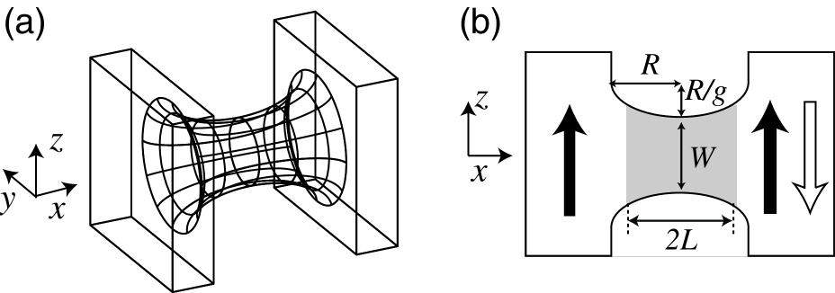
FIG. 1.: (a) The geometry of the constriction potential $V(r_{\parallel},x)$ is schematically shown. (b) The crosssection of the constriction potential in $xz$ plane. Arrows represent the magnetization vectors of electrodes. In the right electrode, the filled (hollow) arrow represents the magnetization vector for the F (A) alignment. The shaded region in the constriction represents the DW with thickness $2L$ for the A alignment.

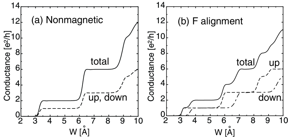
FIG. 2.: (a) The conductance curves for the nonmagnetic PC, $h_{0}=0$, are shown. The total conductance is plotted by the solid line. The conductances for spin-up and spin-down electrons are degenerate and plotted by the dotted line. (b) The conductance curves for the F alignment are shown. The total conductance is indicated by the solid line. The conductance for spin-up (spin-down) electrons is plotted by the dashed (dot-dashed) line. The exchange field is $h_{0}=0.5$ eV.

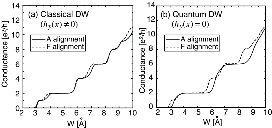
FIG. 3.: (a) The conductance curve for the A (F) alignment with the classical DW is plotted by solid (dotted) linen. (b)The conductance curve for the A (F) alignment with a quantum DW is shown. The spin precession of conduction electron in the quantum DW is forbidden. In both panels, parameters are the same as those in Fig.2 (b)

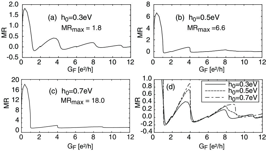
FIG. 4.: The Magnetoresistances(MR) for the PC with $h_{0}=0.3$, 0.5 and 0.7 eV are shown in panels (a), (b) and (c), respectively. The holizontal axis represents the conductance for the F alignment. The enlarged views of MR are shown in the panel (d).

REFERENCES

- [1] J. M. Krans and J. M. van Ruitenbeek, Phys. Rev. B 50, 17659 (1994).
- [2] L. Olesen et al., Phys. Rev. Lett. 72, 2251 (1994).
- [3] G. Rubio et al., Phys. Rev. Lett. 76, 2302 (1996).
- [4] J. L. Costa-Krämer, Phys. Rev. B 55, R4875 (1997).
- [5] M. Büttiker et al., Phys. Rev. B 31, 6207 (1985).
- [6] L. I. Glazman et al., JEPT Lett. 48, 238 (1988).
- [7] A. Yacoby and Y. Imry, Phys. Rev. B 41, 5341 (1990).
- [8] P. Bruno, Phys. Rev. Lett. 83, 2425 (1999).
- [9] M.Julliere, Phys. Lett. 8, 225 (1975).
- [10] S. Maekawa and U. Gäfvert, IEEE Trans. magn. 18, 707 (1982).
- [11] H. Imamura et al., Phys. Rev. B 59, 6017 (1999).
- [12] M. N. Baibich et al., Phys. Rev. Lett. 61, 2472 (1988).
- [13] N. García et al., Phys. Rev. Lett. 82, 2923 (1999).
- [14] H. Oshima and K. Miyano, Appl. Phys. Lett. 73, 2203 (1998).
- [15] T. Ono et al., Appl. Phys. Lett. 75, 1622 (1999).
- [16] K. Hirose and M. Tsukada, Phys. Rev. B 51, 5278 (1995).
- [17] M. Brandbyge et al., Phys. Rev. B 55, 2637 (1997).
- [18] N. Kobayashi et al., Jpn. J. Appl. Phys. 38, 336 (1999).
- [19] J.C.Slonczewski, Phys. Rev. B 39, 6995 (1989).
- [20] P. M. Levy and S. Zhang, Phys. Rev. Lett. 79, 5110 (1997).
- [21] J. F. Gregg et al., Phys. Rev. Lett. 77, 1580 (1996).
- [22] N. D. Lang, Phys. Rev. B 52, 5335 (1995).
- [23] M. Brandbyge et al., Phys. Rev. B 56, 14956 (1997).
- [24] J. C. Cuevas et al., Phys. Rev. Lett. 80, 1066 (1998).
- [25] D. A. Wharam et al., J. Phys. C 21, L209 (1988).
- [26] B. J. van Wees et al., Phys. Rev. Lett. 60, 848 (1988).
- [27] M. Brandbyge, Ph.D. thesis, Technical University of Denmark, 1997.
- [28] R. Schilling, Phys. Rev. B 15, 2700 (1977).
- [29] H. P. Bader and R. Schilling, Phys. Rev. B 19, 3556 (1979).
- [30] L. Berger, J. Apll. Phys. 55, 1954 (1984).
- [31] G. G. Cabrera and L. M. Falicov, Phys. Stat. Sol. (b) 61, 539 (1974).
- [32] J. B. A. N. van Hoof et al., Phys. Rev. B 59, 138 (1999).