[

Magnetic field effects on two-leg Heisenberg antiferromagnetic ladders:
Thermodynamic properties

Abstract

Using the recently developed transfer-matrix renormalization group method, we have studied the thermodynamic properties of two-leg antiferromagnetic ladders in the magnetic field. Based on different behavior of magnetization, we found disordered spin liquid, Luttinger liquid, spin-polarized phases and a classical regime depending on magnetic field and temperature. Our calculations in Luttinger liquid regime suggest that both the divergence of the NMR relaxation rate and the anomalous specific heat behavior observed on Cu₂(C₅H₁₂N₂)₂Cl₄ are due to quasi-one-dimensional effect rather than three-dimensional ordering.

]

Recently spin ladders have been at the focus of intensive research towards understanding the spin-1/2 Heisenberg antiferromagnets in one and two dimensions[1, 2, 3, 4, 5]. Experimentally, several classes of materials like SrCu₂O₃, La₆Ca₈Cu₂₄O₄₁ and Cu₂(C₅H₁₂N₂)₂Cl₄ (CuHpCl) have been found whose properties can be well described by the two-leg Heisenberg antiferromagnetic ladder (THAFL) model[6, 7, 8]. For inorganic oxides, the spin gap $\Delta$ was found around $500K$[9]. So only the low-energy part of spectrum can be explored by measuring spin susceptibility, NMR relaxation and neutron scattering[6, 7, 10]. On the other hand, the organo-metallic compound CuHpCl exhibits a very small spin gap $\Delta$$\approx$$11K$[11] which allows a full investigation of the spectrum by applying a magnetic field (MF). Chaboussant et al. have shown that the NMR relaxation rate exhibits substantially different behavior for different ranges of MF in the low temperature limit. On this basis these authors proposed a magnetic phase diagram[11]. Moreover, the specific heat measurements show anomalous behavior when the spin gap is suppressed by the MF[12, 13]. Theoretically, some of the MF effects on THAFL were discussed by using exact diagonalization, bosonization, conformal field theory and non-linear $\sigma$-model approaches [13, 14, 15, 16, 17, 18, 19]. In this paper, we perform the first calculation of the phase diagram (more precisely crossover lines between different regimes) using the newly developed transfer-matrix renormalization group (TMRG) technique[20]. Our findings suggest the observed divergence of the NMR rate[11] and the anomalous specific heat behavior[12, 13] are due to the MF effects on THAFL i.e., quasi-1D effects rather than 3D field-induced ordering when $H\geq\Delta$.

The Hamiltonian for the THAFL in our studies reads:

$${\cal H} = \sum_{i=1}[J_{\|}({\bf S}_{1,i}\cdot{\bf S}_{1,i+1}+{\bf S}_{2,i}\cdot{\bf S}_{2,i+1})$$ (1)

$$+ J_{\perp}{\bf S}_{1,i}\cdot{\bf S}_{2,i}-H(S_{1,i}^{z}+S_{2,i}^{z})],~{}~{}~{}~{}H>0$$ (2)

where ${\bf S}_{n,i}$ denotes a $S$$=1/2$ spin operator at the $i$-th site of the $n$-th chain. $J_{\|,\bot}$ are the intra- and inter-chain couplings, respectively. To confront the experimental findings on CuHpCl, we set $J_{\|}$$=1$, $J_{\perp}/J_{\|}$$=5.28$.

The TMRG technique we adopt here is implemented in the thermodynamic limit and can be used to evaluate very accurately the thermodynamic quantities [20, 21] as well as imaginary time auto-correlation functions[22, 23] at very low-$T$ for quasi-1D systems. Technical aspects of this method can be found in Ref.[21]. In our calculations, the number of kept optimal states $m=200$, while the width of the imaginary time slice $\epsilon=0.05$ are used in most cases. We have also used different $m$ and $\epsilon$ to verify the accuracy of calculations. The physical quantities presented below are usually calculated down to $T\leq 0.02$ (in units of $J_{\|}$). The lowest temperature reached is $T=0.005$. The relative errors, being different for different quantities, are usually much less than, at most about, one percent for derivative quantities at very low temperatures.

We first determine the spin gap by fitting the spin susceptibility $\chi$, using the asymptotic formula proposed in [24]: $\chi$$=$$A$${\rm e}^{-\Delta/T}/{\sqrt{T}},~{}~{}T\rightarrow 0,$ based on the quadratic dispersion with a gap $\Delta$ for the single magnon branch. Fitting numerical results $\chi$ in the range $T\in[0.168,1]$[25], we obtain $\Delta$$=$$4.385$ which is very close to the value $\Delta$$=$$4.382$ obtained using the $T$$=$$0$ DMRG method (with 250 states kept and extrapolated to infinite size).

FIG. 1.: Magnetization versus $H$ for different $T$

In Fig. 1, we show the magnetization curves for different values of $T\in[0.02,10]$. For quasi-1D spin-gapped systems, it is well-known that at $T=0$, $M=0$ for $H$$\leq$ $H_{C_{1}}$$=$$\Delta$; $M=1$ (in units of $S$) for $H$$\geq$$H_{C_{2}}$$=$$J_{\bot}+2J_{\|}$[8] and $0<M<1$ for $H\in(H_{C_{1}},H_{C_{2}})$. When $T$$\neq$$0$, $M$ is nonzero for any $H$. However, the critical behavior of the magnetization in the vicinity of $H_{C_{1}}$ and $H_{C_{2}}$ can only be seen at very low temperatures. The behavior of $M(H)$ is elucidated in Fig. 2. First consider the $T$$=$$0$ case in (a). We have calculated $M(T$$=$$0)$ at $H=7.275,7.25,7.125,700$ and $4.4,4.5,4.625,4.75$ for the upper and lower critical points, respectively. The calculations for $M(T)$ were done with $m$$=$$256$ down to $T$$\approx$$0.005$ (needed) for extrapolation to $T$$=$$0$ limit. Then fitting $M(T$$=$$0)$ at these $H$ gives the following asymptotic form:

$$M(H)=\left\{\begin{array}[]{ll}0.380\sqrt{H-H_{C_{1}}}{}{}{}&{\rm for}~{}H=H_{C_{1}}^{+}\\ 1-0.431\sqrt{H_{C_{2}}-H}{}{}{}&{\rm for}~{}H=H_{C_{2}}^{-},\end{array}\right.$$ (3)

in agreement with universal square-root singularities of magnetization in gapped systems[26] (see also [15, 17]). Independently, we obtain $H_{C_{1}}=4.3823$ which is even more accurate than the value obtained from fitting $\chi(T)$.

FIG. 2.: (a) Solid lines for the asymptotic behavior Eq. (3). Symbols $\times(+)$ for $T$$=$$0$ at $H$$=$ $H_{C_{1}}^{+}$ $(H_{C_{2}}^{-})$ and up(down) triangles for $T=0.02$ showing the deviation from Eq. (3). (b) ${\rm d}M/{\rm d}H$ vs $H$ (in legends) for $T$$\leq$$T_{0}$; (c) For $T_{0}$$<T$$\leq T_{C}$; (d) For $T$$>$$T_{C}$. In (c) and (d), a constant $\alpha(T)$ is subtracted and derivatives are amplified as seen in parentheses.

When $T$$>$$0$, depending on the behavior of ${\rm d}M/{\rm d}H$, there are three different cases: 1) ${\rm d}M/{\rm d}H$ has a two-peak structure shown in Fig. 2(b) for $T$$<$$T_{0}$$=$$0.59^{+0.04}$ (positive(negative) numbers in super(sub)-scripts are bounds of errors[25]), similar to the $T$$=$$0$ case. 2) It has a single peak structure at $H$$\neq$$0$ in Fig. 2(c) for $T_{0}\leq T$$<$$T_{C}$$=$$4.86_{-0.05}$. 3) It reaches a maximum exactly at $H=0$ for $T$$\geq$$T_{C}$ in Fig. 2(d). Suppose $\gamma$ is the coefficient of the cubic term in the low-$H$ expansion of magnetization, $T_{C}$ is given by $\gamma(T_{C})=0$.

Based on the above observations, we can construct a magnetic phase diagram as shown in Fig. 3. Strictly speaking, quantum phase transitions take place only at $H_{C_{1,2}}$ for $T=0$, and “phase boundaries” are just crossover lines for $T>0$. At $T=0$: 1) as $H<H_{C_{1}}=\Delta$, the band edge of the continuum has $S^{z}_{total}=1$, with an effective gap $\Delta_{eff}^{<}=H_{C_{1}}-H$. The ground state is a disordered spin liquid and thermodynamic quantities decay exponentially at low $T$; 2) As $H_{C_{1}}\leq H\leq H_{C_{2}}$, the gap vanishes and we find a range of linear in $T$ dependence for the specific heat and finite values for the susceptibility, which is characteristic for the Luttinger liquid (LL); 3) The ground state becomes fully polarized when $H>H_{C_{2}}$. There thermodynamic quantities again decay exponentially with $\Delta^{>}_{eff}=H-H_{C_{2}}$ at low $T$. When $T>0$, the LL regime shrinks gradually and disappears at $T=T_{0}$ and $H=H_{m}$, beyond which the system “forgets” about $H_{C_{1}},H_{C_{2}}$ and $\Delta$[27]. The other two phases continue to exist until $T=T_{C}$, and one finds a classical regime for $T>T_{C}$.

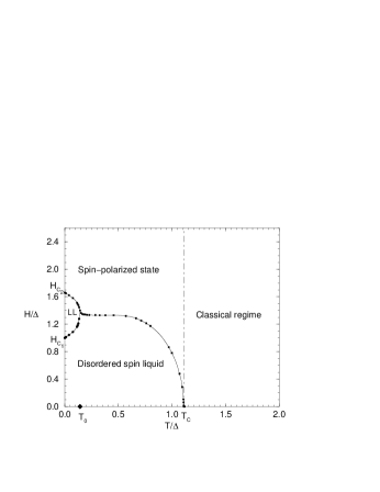
FIG. 3.: Magnetic phase diagram: the dots fitted by lines as phase boundary in-between the LL, the spin-polarized phase and the disordered spin liquid, indicate values of $H$ and $T$ maximizing ${\rm d}M/{\rm d}H$.

Compared with the phase diagram proposed on the basis of $1/T_{1}$ measurements[11], the major difference is the absence of the “quantum critical” phase in Fig. 3. We note that the requirement for exhibiting the universal “quantum critical” behavior $J\gg\Delta$ [28] is not satisfied in our case. In addition, for the classical regime, we found $T_{C}=1.109_{-0.011}\Delta$ instead of $T_{C}=\Delta$. In Ref. [11], the phase boundaries for the quantum critical phase with two gapped phases are given as the onset of the exponential behavior in $1/T_{1}$ at $T=\Delta^{>,<}_{eff}$. (Consequently, one obtains $H=H_{C_{1,2}}$ at $T=0$ and $T_{C}=\Delta$ from $\Delta^{<}_{eff}=0$ at $H=0$.) The divergence of $1/T_{1}$ presumably disappears at the boundary of the LL regime. In fact, $1/T_{1}$ has contributions from magnon scattering with momentum transfer of both $q=0$ and $q=\pi$. The former process corresponds to a larger gap in the continuum, but contributes substantially to the relaxation[29]. In our calculations the critical behavior of $M(H)$ defining the quantum phase transitions is identified directly at $T=0$. When $T>0$, a straightforward extension of this definition gives rise to all regimes except for the “quantum critical” phase. We should also mention that when $J_{\bot}\rightarrow 0$, one has $\Delta\rightarrow 0$, $T_{0}\rightarrow T_{C}$ and $H_{m}\rightarrow 0$.

Now elaborate more on the temperature dependence of $M(T)$ for various given $H$ as shown in Fig. 4. Consider a cooling process. For $T>T_{C}\approx\Delta$, $M$ monotonically but slowly increases for all $H$, whereas it can change non-monotonically depending upon the values of $H$ for $T<T_{C}$. When $H$$>$$H_{C_{2}}$, $M$ continues to increase and saturates exponentially with $\Delta_{eff}^{>}$. However, when $H$$<$$H_{C_{1}}$, $M$ first goes up, then down and finally decays to zero exponentially with $\Delta_{eff}^{<}$. When $H_{C_{1}}<H<H_{C_{2}}$, there is always a maximum at $T\neq 0$, close to the boundary between the polarized phase and LL for $H\geq H_{m}\approx 6$[25], while separating the former from the disordered spin liquid phase elsewhere. There is also a minimum for LL. The positions of minima are at $T=0$ for $H\geq H_{m}$, otherwise they are close to the boundary of the LL regime.

FIG. 4.: Magnetization vs. temperature: curves for $H$ $=$ $9,$ $8,$ $7.415,$ $7.28,$ $7.125,$ $7,$ $6.75,$ $6.25,$ $6,$ $5.75,$ $5.5,$ $5,$ $4.625,$ $4.5,$ $4.385,$ $4.125,$ $3.5$ from top to bottom. Symbols $\bigtriangleup$ ($\bigtriangledown$) denote maxima (minima) at each $H$. Extra points added between curves are for maxima at $7.25,$ $5.875,$ $5.812,$ $2,$ $1,$ $0.005$ and minima at $5.875,$ $5.812$.

The origin of this nontrivial temperature dependence, in particular, the presence of minima and maxima at low temperatures, is not fully understood. One possible interpretation is due to the excitation spectrum in the presence of MF. $S^{z}_{total}$ is a good quantum number for the Hamiltonian (2 ) and thus different energy bands are shifted by $-S^{z}_{total}H$. When $H<H_{C_{2}}$, the ground state is not a fully polarized state(FPS), but the low-lying excitations correspond to positive $S_{total}^{z}$, and the maximum, roughly speaking, corresponds to the “maximally polarized” state. This is true so far $H$$>$$H_{m}$. On the other hand, the minimum at $T$$\neq$$0$ originates from low-lying states in $S_{tot}^{z}$$=$$0$ subspace. Those states intersect with FPS at $H=H_{m}$. Notably, $H_{m}$ also corresponds to an extrapolation of the boundary between the two gapped phases in the phase diagram ( Fig.3). It is also curious to note that in Fig. 4, the curves are roughly symmetric w.r.t. $M=0.5$, if we focus on the low temperature part. This reflects the particle-hole symmetry of the problem in the fermion representation[15, 11].

We now turn to the specific heat which, similar to $M(T)$, shows different behavior depending on $H$. When $H<H_{C_{1}}$ in Fig. 5(a), $C_{v}$ has a single peak structure as expected. The MF reduces $\Delta_{eff}^{<}$, and changes dramatically the line shape near $T=0.5$, as $H\rightarrow H_{C_{1}}^{-}$. This is a signature of approaching the quantum critical point[28]. When $H_{C_{1}}$$<H$$<H_{C_{2}}$ in Fig. 5(b) and (d), a second peak at low $T$ is developed exhibiting the LL behavior. Linear-$T$ dependence is shown in the insets of (b) and (d). Moreover, at $H=H_{C_{1}}^{+}$, the cusp still remains and at $H=H_{C_{2}}^{-}$ a shoulder emerges. When $H\geq H_{C_{2}}$ in Fig. 5(c), the shoulder can still be seen for $H=H_{C_{2}}^{+}$, although the second peak vanishes. At low-$T$, $C_{v}$ decreases exponentially with $\Delta_{eff}^{>}$. We note the cusps and shoulders appear outside the LL regime but at the vicinity of its boundary. For those $H$ at which a larger second peak shows up, the local minima are also located outside the LL regime, but nearby.

FIG. 5.: Specific heat at various $H$ (legends): For $H<H_{C_{1}}$ in (a); $H_{C_{1}}<H<H_{C_{2}}$ in (b) and (d); $H\geq H_{C_{2}}$ in (c). Insets for low-T behavior: $C_{v}$ in (a)-(d) and $C_{v}/T$ in (b) and (d). Triangles denote maximum $C_{v}$.

It is also instructive to see the MF effects on the maximum specific heat $C^{max}_{v}$ and corresponding temperature $T_{max}$. As seen in Fig. 6, when $H$ is applied, $C_{v}^{max}$ first declines as a gradual response to the splitting. At $H=H_{m}$, because of the crossing of two kinds of energy states discussed above, $C^{max}_{v}$ arrives at a minimum. Moreover, we surprisingly found that the curvature of $T_{max}$ changes its sign at $H_{C_{1}}$, while it reaches a maximum at $H=H_{C_{2}}$. These interesting features show an intrinsic aspect of the MF effects as demonstrated consistently by the magnetization and the specific heat.

Finally we discuss the bearings of our numerical results on experimental findings of a diverging NMR relaxation rate and peculiar specific heat behavior. Recently, Chaboussant et al. found that the NMR rate anomalously increases for $H_{C_{1}}$$\leq$$H$$\leq$$H_{C_{2}}$ when $T$ decreases[11]. These authors attributed this anomalous increase to quasi-1D behavior. Our results show that it is indeed an intrinsic MF effect on the spin ladders. In fact, the increasing of the NMR rate starts already at the vicinity of the LL regime which is bounded by $T$$\approx$$1.6K$. This should share the same physical origin as the occurrence of the cusps and shoulders for $C_{v}$ at the vicinity of the LL regime. On the other hand, Hammar et al.[12] have measured $C_{v}$ up to $H=9$T, which is about $(5.10\pm 0.17)J_{\|}$, taking into account the difference between the experimental and numerical results for the gap due to other interactions[14, 11]. As seen in Fig. 3 of Ref. [12], the overall feature is consistent with our results in Fig. 5(a) and (b), e.g. the shift of $C_{v}^{max}$ and $T_{max}$ as well as the abrupt change for $H$$=$$6.6$T. The development of the shoulder and the second peak at low temperatures is clearly seen in more recent measurements [13] in full agreement with our calculations. When $H_{C_{1}}$$<$$H$$<$$H_{C_{2}}$, we notice that a narrow subpeak emerges from the second peak at lower temperature (see Fig. 2(b) of Ref. [13]). The subpeak might indicate the on-set of the 3D effects [12, 13], while the second peak represents the magnetic effects on the THAFL. On contrary, the NMR rate changes smoothly versus temperature in the LL regime. Therefore, the anomalous behavior of the NMR rate results from the magnetic effects of THAFL as a characteristic feature of quasi-1D gap systems.

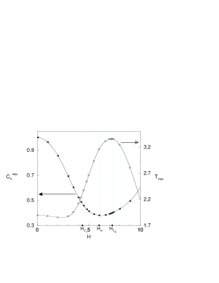
FIG. 6.: The maximum specific heat $C_{v}^{max}$ (to the left) and the corresponding temperature $T_{max}$ (to the right) versus $H$.

In conclusion, we have proposed a magnetic phase diagram for the two-leg ladders. We emphasize that most of the striking MF effects show up in the LL regime, giving rise to the divergence of the NMR rate and anomalous specific heat observed in experiments. Moreover, this magnetic phase diagram is generically valid for other spin-gapped systems as well and the results on $M(T)$ should also shed some light on other quasi-one dimensional fermion systems which involve either a charge gap or a band gap, with $H$ replaced by the chemical potential.

We are grateful to D. Loss, A.A. Nersesyan, T.K. Ng, B. Normand and Z.B. Su for fruitful discussions and to G. Chaboussant for helpful correspondence.

REFERENCES

- [1] E. Dagotto and T.M. Rice, Science, 271, 618(1996).
- [2] E. Dagotto, J. Riera, D.J. Scalapino, Phys. Rev. B 45, 5744(1992).
- [3] T.M. Rice, S. Goplan and M. Sigrist, Europhs. Lett. 23, 445(1993); M. Sigrist, T.M. Rice and F.C. Zhang, Phys. Rev. B 49, 12058(1994).
- [4] T. Barnes and J. Riera, Phys. Rev. B 50, 6817 (1994).
- [5] X. Wang, cond-mat/9803290.
- [6] M. Azuma, Z. Hiroi and M. Takano, Phys. Rev. Lett. 73, 3463(1994).
- [7] T. Imai K.R. Thurber, K.M. Shen, A.W. Hunt and F.C. Chou, Phys. Rev. Lett. 81 220 (1998).
- [8] G. Chaboussant, P.A. Crowell, L.P. Lévy, O. Piovesana, A. Madouri, and D. Mailly, Phys. Rev. B 55, (1997) 3046.
- [9] D.C. Johnston, Phys. Rev. B 54, 13009 (1996).
- [10] R. Eccleston, M. Uehara, J. Akimitsu, H. Eisaki, N. Motoyama and S. Uchida, Phys. Rev. Lett. 81, 1702 (1998).
- [11] G. Chaboussant, Y. Fagot-Revurat, M.-H. Julien, M.E. Hanson, C.Berthier, M. Horvatić, L.P. Lévy and O. Piovesana, Phys. Rev. Lett 80 2713 (1998); Euro. Phys. Jour. B 6,167 (1998).
- [12] P.H. Hammar, D.H. Reich, C. Broholm and F. Trouw, Phys. Rev. B 57, 7846 (1998).
- [13] R. Calemczuk, J. Riera, D. Poiblanc, J.-P. Boucher, G.Chaboussant, L. Lévy, and O. Piovesana, Euro. Phys. Jour. B 7, 171 (1999).
- [14] C. Hawyard, D. Poilblanc and L.P. Lévy, Phys. Rev. 54, (1996) 12649.
- [15] R. Chitra and T. Giamarchi, Phys. Rev. B 55, 5816 (1997).
- [16] M. Usami and S. Suga, Phys. Rev. B 58 14401 (1998).
- [17] T. Sakai and M. Takahashi, Phys. Rev. B 57, 8091 (1998).
- [18] B. Norman, J. Kyriakidis, D. Loss, cond-mat/9902104.
- [19] T. Giamarchi and A. M. Tsvelik, Phys. Rev. B 59, 11398(1998).
- [20] R.J. Bursill. T. Xiang, and G.A. Gehring, J. Phys.: Condens. Matter 8, L583 (1996); X. Wang and T. Xiang, Phys. Rev. B 56, 56 (1997).
- [21] T. Xiang and X. Wang, Density-Matrix Renormalization, Lecture Notes in Physics vol. 528, edited by I. Peschel, X .Wang, M Kaulke, and K. Hallberg, (Springer-Verlag, New York, 1999).
- [22] T. Mutou, N. Shibata and K. Ueda, Phys. Rev. Lett. 81, 4939 (1998).
- [23] F. Naef, X. Wang, X. Zotos and W. von der Linden, Phys. Rev. B 60, 359 (1999).
- [24] M. Troyer, H. Tsunetsugu and D. Würtz, Phys. Rev. B 50, 13515 (1994).
- [25] The detail will be discussed elsewhere.
- [26] G. I. Japaridze and A. A. Nersesyan, JETP Lett. 27, 334 (1978); V.L. Pokrovsky and A.L. Talapov, Phys. Rev. Lett. 42, 65 (1979).
- [27] In Matsubara Green functions gap is compared with , and , very close to in our case. This remark is due to A.A. Nersesyan.
- [28] J.A. Hertz, Phys. Rev. B 14, 1165 (1976); S. Sachdev, Phys. Rev. B 55, 142 (1997); Quantum Phase Transitions, Cambridge U. Press, 1999.
- [29] F. Naef and X. Wang, Phys. Rev. Lett., to appear.