The absorption of bulk acoustic phonons in a two-dimensional (2D) GaAs/AlGaAs heterostructure is studied (in the clean limit) where the 2D electron-gas (2DEG), being in an odd-integer quantum-Hall state, is in fact a spin dielectric. Of the two channels of phonon absorption associated with excitation of spin waves, one, which is due to the spin-orbit (SO) coupling of electrons, involves a change of the spin state of the system and the other does not. We show that the phonon-absorption rate corresponding to the former channel (in the paper designated as the second absorption channel) is finite at zero temperature ($T$), whereas that corresponding to the latter (designated as the first channel) vanishes for $T\to 0$. The long-wavelength limit, being the special case of the first absorption channel, corresponds to sound (bulk and surface) attenuation by the 2DEG. At the same time, the ballistic phonon propagation and heat absorption are determined by both channels. The 2DEG overheat and the attendant spin-state change are found under the conditions of permanent nonequilibrium phonon pumping.

             PACS: 73.40.Hm, 63.22.+m, 71.70.Ej, 75.30.Fv

I Introduction

In recent years considerable amount of interest has been focused on the problem of the acoustic wave and heat absorption by a 2DEG in GaAs/AlGaAs-heterostructures in the quantum Hall regime (QHR) [1, 2, 3, 4, 5, 6, 7, 8, 9, 10, 11, 12]. This is connected with the search for a new way to study the fundamental properties of a 2DEG in a strong magnetic field (which is considered to be perpendicular to the layer, i.e., $\mbox{\boldmath$B$}\parallel{\hat{z}}$) employing nonequilibrium phonons [2, 3] or surface acoustic waves [4, 5, 6, 7, 8, 9] as an experimental tool. The basic idea is associated with the fact that the energies of phonons generated by heated metal films [2, 3, 13] or the energy of coherent phonons in semiconductor superlattices [14] may be of the order of the characteristic gaps in the 2DEG spectrum. At the same time, it is well-known that in the QHR a change of the Landau level (LL) filling factor $\nu$ may drastically renormalize the 2DEG excitation spectrum. Therefore parameters such as the phonon life-time (PLT) $\tau_{\mbox{ph}}$, the attenuation, and the velocity of sound waves exhibit strong oscillations as functions of the applied magnetic field [1, 4, 5, 6, 7, 8, 9]. These spectrum alterations prevent development of an universal approach to the theoretical problem of sound and heat absorption by 2DEG.

Most of the relevant treatments[10, 11, 12, 15] use the one-particle approximation, i.e. the Coulomb electron–electron ($e$-$e$) interaction is neglected or considered as a secondary phenomenon renormalizing the phonon displacement field (screening in Ref. [12]) or one-electron state density (Coulomb gap in Ref. [15]). In these studies the LL width is determined by the amplitude $\Delta$ of the smooth random potential (SRP), and the phonon absorption occurs through the transition of an electron from one semiclassical trajectory to another in the SRP field near the percolation threshold[11, 12] (when $\nu$ is close to a half-integer) or by the electron variable-range hopping for strongly localized electrons[15] ($\nu$ is close to an integer). The one-particle approximation is evidently justified in a qualitative sense as long as the number of charged quasiparticles is rather large, which does not hold in the integer (or “almost” integer) QHR. In this latter case one should take into account a strong $e$-$e$ interaction with the typical energy equal to the Coulomb energy $E_{C}\sim e^{2}/\varepsilon\l_{B}$ ($\varepsilon$ is the dielectric constant, $l_{B}=(\hbar c/eB)^{1/2}$ is the magnetic length), which exceeds 100 K for $B>8\,$T. Since we have $E_{C}/\Delta\,\raise 1.72218pt\hbox{$>$}\kern-8.00003pt\lower 3.01385pt\hbox{$\sim$}\,10$ and because of the absence of charged quasiparticles in the ground state, it is exactly $E_{C}$ that determines the real LL width in the integer QHR. Charge excitations are separated from the ground state, not only by the gap, which is equal to the Zeeman energy for odd $\nu$ or the cyclotron energy $\hbar\omega_{c}$ for even $\nu$, but also by an additional energy of order $E_{C}$. This applies also to the so-called skyrmion charge excitations[16, 17, 18], which seem to have been observed[19, 20] at $\nu=1$. However, if $\nu$ deviates from unity then even the ground state has to be realized as a complex spin and charge texture in the form of a Skyrme crystal with a characteristic period proportional to ${|\nu-1|}^{-1/2}$ (see Refs. [16, 21, 22]), so that ignoring the skyrmions is only permissible for $\nu$ close enough to unity. Experiments[19, 20] indicate that this can indeed be done if $|\nu-1|\,\raise 1.72218pt\hbox{$<$}\kern-8.00003pt\lower 3.01385pt\hbox{$\sim$}\,0.01$.

Therefore in integer QHR the phonon absorption by chargeless excitations has to be more efficient. The spectrum calculation for low energy excitations from the filled LL is fortunately an exactly solvable problem to first order in $E_{C}/\hbar\omega_{c}$, which is considered to be small (see Refs. [23, 24]). We will study the odd $\nu$ only, since at even $\nu$ the cyclotron gap for excitations substantially exceeds the possible acoustic phonon energy. For $\nu=2n+1$ when the $n$-th LL in the ground state has a fully occupied lower spin sublevel and an empty upper one the lowest states in the spectrum are spin excitons, which are in fact spin wave excitations. We will call these simply spin waves (SWs). For them the gap is $|g\mu_{b}B|\approx 0.3B\,$K/T, because $g=-0.44$ for GaAs. At temperatures $T\,\raise 1.72218pt\hbox{$>$}\kern-8.00003pt\lower 3.01385pt\hbox{$\sim$}\,0.1\,$ an appreciable amount of “thermal” SWs forms a rarefied 2D Bose gas, since SW density is still far less than the density of electrons in the $n$-th LL (i.e., than $1/2\pi l_{B}^{2}$). As a result, the electron–phonon ($e$-$ph$) interaction can be represented as the SW–phonon interaction. Such a representation for the $e$-$ph$ interaction Hamiltonian has already been found earlier[26] (see also Sec. 2 of the present paper), and as discussed it includes, in addition to spin-independent terms, the small terms arising from the electron SO coupling. Precisely the latter ones determine the phonon absorption at $T=0$.

We consider two channels of inelastic phonon scattering. The first one (Sec. 3 of the present paper) does not change the 2DEG spin state. The rate of phonon absorption is proportional to the conserved number of equilibrium SWs and vanishes when $T$ goes to zero. Therefore, as the 2DEG temperature due to phonon absorption increases the SWs chemical potential has to decrease in this case. After averaging with a certain phonon distribution over the momenta we find the mean effective inverse PLT $1/\tau_{\mbox{eff}}$, and hence the rate of the 2DEG heating as well as the corresponding contribution to the inverse thermal conductivity. The transition to the limit $kl_{B}\ll 1$ ($\mbox{\boldmath$k$}=(\mbox{\boldmath$q$},k_{z})$ is the phonon wave vector) allows one to find the “2D” contribution to the bulk and surface acoustic wave attenuation. In this last case the piezoelectric electron–lattice interaction plays the main role.

The second phonon absorption channel (Sec. 4) arises from the SO coupling. It describes the SW generation from the 2DEG ground state. Absorption of a single phonon reduces by 1 both the spin component $S_{z}$ and the total electron-spin number $S$. As a consequence, the absorption rate is proportional to the rate of spin momentum decrease. This channel of scattering which is pinched off for energies less than the Zeeman energy gap, is only accessible for a selected group of “resonant” phonons with a certain kinematic relationship between $q$ and $k_{z}$ wave vector components. Of course, the long-range wave limit is meaningless in this case. While the phonons of the resonant group occupy a comparatively small phase volume in $k$-space, their contribution to the effective inverse PLT is rather significant and, being independent of temperature, can exceed the corresponding contribution from the first absorption channel even at $T\,\raise 1.72218pt\hbox{$<$}\kern-8.00003pt\lower 3.01385pt\hbox{$\sim$}\,1\,$K.

In Section 5 we consider both absorption channels in the problem of dynamic quasi-equilibrium in a 2DEG under the condition of ballistic phonon pumping. We find the dependence of the final temperature as well as the spin momentum of the 2DEG on the initial temperature of the 2DEG and the density of the nonequilibrium phonons. We note in passing that the 2DEG adds a small correction to the bulk phonon scattering, connected mainly with the lattice defects and sample boundaries. One can also get only a small (although peculiar) 2DEG correction to the thermal conductance[1, 10]. The 2DEG contribution to the phonon absorption always contains the factor $1/L_{z}$ ($L_{z}$ is the sample thickness in the ${\hat{z}}$ direction) in the expression for the value of $1/\tau_{\mbox{ph}}$. We assume that the distribution of the nonequilibrium phonons in $k$-space and the amplitude of the sound wave in the 2D channel, which are determined by the acoustic-phonon scattering, to be known.

In closing this Section we should like to mention the SRP role specifically in the case of the studied problem. The ground state in the clean limit with strictly odd $\nu$, being built of one-electron states of the fully occupied lower spin sublevel (see Refs. [23, 24, 26, 27]), is actually the same as for the 2DEG without Coulomb interaction. Accordingly, the ground state in the presence of SRP is of the same nature. Note that the SRP would give rise to free charged quasiparticles, were it not that the loss in energy due to interaction (which is on the order of $|g\mu_{b}B|+E_{C}$), was vastly in excess of the gain $\Delta$ in energy due to fluctuations in the random potential[28]. We have no free quasiparticles at temperatures $T\ll E_{C}$, and such a 2DEG is a spin dielectric. Furthermore the neutral spin exciton with 2D momentum $\hbar{\mbox{\boldmath$q$}}_{\mbox{ex}}$ has a dipole momentum $el_{B}^{2}\mbox{\boldmath$q$}_{\mbox{ex}}\times{\hat{z}}$ (see Refs. [23, 24, 25]) and in SRP the exciton may gain an energy on order $l_{B}^{2}q_{\mbox{ex}}\Delta/\Lambda$ in the dipole approximation, where $\Lambda$ is SRP correlation length. The associated loss is the “kinetic” energy $(q_{\mbox{ex}}l_{B})^{2}/2M$ ($M\sim E_{C}^{-1}$ is the excitonic mass[23, 24, 25]). Therefore for $q_{\mbox{ex}}\,\raise 1.72218pt\hbox{$<$}\kern-8.00003pt\lower 3.01385pt\hbox{$\sim$}\,q_{0}=\Lambda^{-1}\Delta M\sim\Delta/E_{C}\Lambda$ one has to take into account the SRP effect on the SW energy. Our approach to the phonon absorption by the equilibrium SWs ignores the presence of SRP in the system, so it is only correct for temperatures $T>(q_{0}l_{B})^{2}/2M\sim 10\,$mK (this estimate has been done for $B=10\,$T, $\Delta=1\,$meV, and $\Lambda=50\,$nm).

II One-exciton states and the electron–phonon Interaction Hamiltonian in the Excitonic Representation

In this Section we introduce the so-called ‘excitonic representation’ of the Hamiltonian, and its eigenstates, describing the 2DEG under consideration. Let $a_{p}$ and $b_{p}$ be annihilation operators for an electron in the Landau gauge state $\Psi_{p}(x,y)=L^{-1/2}e^{ipy}\psi_{n}(pl_{B}^{2}+x)$ at the lower and upper spin sublevels, respectively. Here $L\times L$ is the size of the 2D system, and $\psi_{n}$ is the $n$-th harmonic oscillator function. In the “one-exciton”approximation, the absorption of one phonon which is not accompanied by a change in the spin state of the 2DEG amounts to a transition between the one-spin-wave states of the 2DEG. The one-spin-wave state with 2D momentum $\hbar\mbox{\boldmath$q$}$ is defined as

$$|\mbox{\boldmath$q$}\rangle=Q^{+}_{\bf q}|0\rangle\,.$$

Here the creation operator for SW,

$$Q_{\bf q}^{+}={\cal N}^{-1/2}\sum_{p}\,e^{-iq_{x}p}b_{p+\frac{q_{y}}{2}}^{+}\,a_{p-\frac{q_{y}}{2}}\,,$$

operates on the 2DEG ground state $|0\rangle$, and ${\cal N}={L^{2}}/{2\pi l_{B}^{2}}$ is the number of magnetic flux quanta, or equivalently, the number of electrons in the $n$-th LL. The equations

$$a^{+}_{p}|0\rangle=b_{p}|0\rangle\equiv 0\quad\mbox{for any $p$},$$

may be regarded as the definition for $|0\rangle$. The main aspect of the excitonic representation is that the state (2.1) is an eigenstate of the full electron Hamiltonian ${\cal H}$ involving the $e$-$e$ interaction: ${\cal H}|\mbox{\boldmath$q$}_{\mbox{ex}}\rangle=[E_{0}+\epsilon(\mbox{\boldmath$q$}_{\mbox{ex}})]|\mbox{\boldmath$q$}_{\mbox{ex}}\rangle$ ($E_{0}$ is the 2DEG ground state energy and $\epsilon(\mbox{\boldmath$q$}_{\mbox{ex}})$ is the SW energy). Of course, this is valid to first order in $E_{c}/\hbar\omega_{c}$ and in the 2D limit (we assume that $d<l_{B}<r_{b}$, where $r_{b}$ is the Bohr radius in the material and $d$ is the effective 2DEG thickness). In the limit $q_{\mbox{ex}}l_{B}\ll 1$ appropriate to our problem one may use the quadratic approximation for the excitonic energy,

$$\epsilon(q_{\mbox{ex}})=\delta+\frac{(q_{\mbox{ex}}l_{B})^{2}}{2M}\,,$$

where

$$\delta=|g\mu_{b}B|\,,$$

and

$$\quad M^{-1}=l_{B}^{2}\int_{0}^{\infty}\frac{p^{3}dp}{4\pi}V(p)e^{-p^{2}l_{B}^{2}/2}[L_{n}(p^{2}l_{B}^{2}/2)]^{2}$$

($L_{n}$ is the $n$-th order Laguerre polynomial), which is defined in terms of the Fourier components $V(q)$ of the Coulomb potential in the heterostructure averaged over the 2DEG thickness[26, 27]. Note that $1/M\sim E_{c}$ holds, besides our results depend on the LL number $n$ only because the excitonic mass (2.6) depends on $n$.

The excitonic representation for the interacting Hamiltonian involves the displacement operators:

$${A_{\bf q}^{+}\choose B_{\bf q}^{+}}={A_{-{\bf q}}\choose B_{-{\bf q}}}=\frac{1}{\cal N}\sum_{p}e^{-iq_{x}p}{a_{p+\frac{q_{y}}{2}}^{+}a_{p-\frac{q_{y}}{2}}\choose b_{p+\frac{q_{y}}{2}}^{+}b_{p-\frac{q_{y}}{2}}}\,.$$

The identities in (2.3) can be rewritten in the excitonic representation as

$$A^{+}_{\bf q}|0\rangle\equiv\delta_{0,{\bf q}}|0\rangle,\quad B^{+}_{\bf q}|0\rangle=Q_{\bf q}|0\rangle\equiv 0\,.$$

The operator in Eq. (2.2) (as well as its Hermitian conjugate) seems to have been first introduced in Ref. [29]. Later some of its combinations together with the operators (2.7) were in fact used as the “valley wave”[30, 31] or “iso-spin”[21] operators. In Ref. [26] the operators (2.2) and (2.7) have been considered exactly in the present form. In what follows, we shall take advantage of the commutation relations

$$e^{-i\Theta_{12}}[A_{{\bf q}_{1}}^{+},Q^{+}_{{\bf q}_{2}}]=-e^{i\Theta_{12}}[B_{{\bf q}_{1}}^{+},Q^{+}_{{\bf q}_{2}}]=-{\cal N}^{-1}Q^{+}_{{\bf q}_{1}\!+\!{\bf q}_{2}}\,,$$

and

$$[Q_{{\bf q}_{1}},Q_{{\bf q}_{2}}^{+}]=e^{i\Theta_{12}}A_{{\bf q}_{1}\!-\!{\bf q}_{2}}-e^{-i\Theta_{12}}B_{{\bf q}_{1}\!-\!{\bf q}_{2}}\,,$$

where $\Theta_{12}=l_{B}^{2}(\mbox{\boldmath$q$}_{1}\times\mbox{\boldmath$q$}_{2})_{z}/2$.

The $e$-$ph$ interaction Hamiltonian is presented as (see, e.g., Refs.[10, 26]):

$${\cal H}_{\mbox{e,ph}}=\frac{1}{L}\left(\frac{\hbar}{L_{z}}\right)^{1/2}\,\sum_{{\bf q},{k}_{z},s}{U^{\prime}}_{s}(\mbox{\boldmath$k$})\,P_{{\bf k},s}H_{\mbox{e,ph}}(\mbox{\boldmath$q$})\qquad+\qquad\mbox{H.~{}c.}\,,$$

where $P_{{\bf k},s}$ is the phonon annihilation operator (index $s$ denotes the polarization state, with $s=l$ denoting the longitudinal and $s=t$ the transversal polarization state). The $H_{\mbox{e,ph}}$ operates on the electron states, and ${U^{\prime}}_{s}(\mbox{\boldmath$k$})$ is the renormalized vertex which includes the fields of deformation (DA) and piezoelectric (PA) interactions. The integration with respect to $z$ has been already performed, and reduces to the renormalization ${U^{\prime}}_{s}(\mbox{\boldmath$k$})=\gamma(k_{z})U_{s}(\mbox{\boldmath$k$})$, where the formfactor

$$\gamma(k_{z})=\int f^{*}(z)e^{ik_{z}z}f(z)\,dz$$

is determined by the wave function $f(z)$ of the corresponding size-quantized level (which we have assumed to be identical for all ${\cal N}$ electrons). For the three-dimensional (3D) vertex one needs only the expressions for the squares,

$$|U_{s}|^{2}=\pi\hbar\omega_{s,k}/p_{0}^{3}\tau_{A,s}(\mbox{\boldmath$k$})\,,$$

where $\omega_{s,k}=c_{s}k$ are the phonon frequencies, $p_{0}=2.52\cdot 10^{6}\,$cm^-1 is the material parameter of GaAs (Ref. [32]), and $c_{l}$ and $c_{t}$ are the sound velocities. The longitudinal $\tau_{A,l}(\mbox{\boldmath$k$})$ and transverse $\tau_{A,t}(\mbox{\boldmath$k$})$ times are 3D acoustic phonon life-times (see Appendix I). These quantities are expressed in terms of nominal times $\tau_{D}=0.8\,$ps and $\tau_{P}=35\,$ps characterizing respectively DA and PA phonon scattering in three-dimensional GaAs crystal. (See Ref. [26] and cf. Ref. [32].)

Initially, of course, the originally spin-independent Hamiltonian of the $e$-$ph$ interaction (2.11) is used. However it does not commute with the SO coupling part of the electron Hamiltonian. Therefore the operator $H_{\mbox{e,ph}}$ including the relevant off-diagonal corrections in the excitonic representation has the following form[26] (we write it for $ql_{B}\ll 1$):

$$H_{\mbox{e,ph}}(\mbox{\boldmath$q$})=\left\{{\cal N}(A_{\bf q}^{+}+B_{\bf q}^{+})\right.\quad{}\qquad{}\qquad{}$$

$${}\qquad{}\qquad{}+\left.{\cal N}^{1/2}l_{B}\left[(vq_{-}-iuq_{+})Q_{-{\bf q}}-(iuq_{-}+vq_{+})Q_{\bf q}^{+}\right]\right\}\,,$$

where $q_{\pm}=\mp i2^{-1/2}(q_{x}\pm iq_{y})$. Here $u$ and $v$ are dimensionless parameters (just as in Ref. [26]) characterizing the SO coupling. The terms containing the coefficient $v$ originate from the absence of inversion in the direction perpendicular to the 2D layer and hence $v$ is proportional to the strength of the normal electric field in the heterostructure[33]. The terms including $u$ are related to the lifting of spin degeneracy for the $S$-band in A₃B₅ crystals[34]. In deriving Eq. (2.14), we have assumed that the normal ${\hat{z}}$ is parallel to the principal [001] axis of the crystal. The final results depend only on the combination $u^{2}+v^{2}$, which is of order $10^{-5}$ for $B=10\,$T with $d=5\,$nm and is proportional to $B^{-1}$ and also to $d^{-4}$ in the asymptotic limit $d\to 0$.

Further in our estimations we proceed from the fields $B\simeq 5\div 20\,$T, and so $\delta$ (2.5) has the same order of magnitude as $\hbar c_{s}/l_{B}$ (precisely $l_{B}\simeq 6\div 11\,$nm,${}\quad\delta\simeq 1.5\div 6\,\mbox{K},\quad\hbar c_{l}l_{B}^{-1}\simeq\ 3\div 7\,\mbox{K},\quad\hbar c_{t}l_{B}^{-1}\simeq 2\div 4\,\mbox{K}$). The magnitude of the exciton mass depends on the layer thickness according to Eq. (2.6) because $V(q)$ depends on the size-quantized function $f(z)$; for real heterostructures $M^{-1}\simeq 40\div 80\,$K.

Note also that everywhere below, the specific magnetic-field dependence of our results is given at constant $\nu$, i.e., the surface electron density is always considered to be proportional to $B$.

III Phonon absorption without a change of the spin state (the first absorption channel)

Considering for the present the first absorption channel, we find the PLT from the well known formula

$$\frac{1}{\tau_{s}(\mbox{\boldmath$k$})}=\sum_{i\neq f}W_{if}(\mbox{\boldmath$k$})[b_{T}(\epsilon_{i})-b_{T}(\epsilon_{f})],$$

where the scattering probability

$$W_{if}(\mbox{\boldmath$k$})=\frac{2\pi}{\hbar}|{\cal M}_{if}^{s,{\bf k}}|^{2}\delta(\epsilon_{i}-\epsilon_{f}+\hbar\omega_{s,k})$$

contains the matrix element of the Hamiltonian (2.11) (Ref. [35]). The value of ${\cal M}_{if}^{s,{\bf k}}$ is determined by the annihilation of one phonon having momentum $\hbar\mbox{\boldmath$k$}$ and by the transition of the 2DEG between the states $|i\rangle=|\mbox{\boldmath$q$}_{\mbox{ex}}\rangle$ and $\langle f|=\langle\mbox{\boldmath$q$}_{\mbox{ex}}\!+\!\mbox{\boldmath$q$}|$, where $q$ is the component of $k$ in the 2DEG plane (for the analogous formulae for phonon absorption by free electrons, see, e.g., Refs. [10, 12, 32]). Here $\epsilon_{i}=\epsilon(\mbox{\boldmath$q$}_{\mbox{ex}})$ and $\epsilon_{f}=\epsilon(\mbox{\boldmath$q$}_{\mbox{ex}}+\mbox{\boldmath$q$})$ and the function $b_{T}(\epsilon)$ in Eq. (3.1) corresponds to the Bose distribution for SWs,

$$b_{T}(\epsilon)=\frac{1}{\exp{[(\epsilon-\mu)/T]}-1}\,,\qquad\mbox{where}\qquad\mu<\delta\,.$$

According to Eqs. (2.11) and (2.14) the square of the modulus is

$$|{\cal M}_{if}^{s,{\bf k}}|^{2}=\frac{\pi|\gamma(k_{z})|^{2}\hbar^{2}\omega_{s,k}}{p_{0}^{3}L^{2}L_{z}\tau_{A,s}(\mbox{\boldmath$k$})}\left|\langle\mbox{\boldmath$q$}_{\mbox{ex}}+\mbox{\boldmath$q$}|H_{\mbox{e,ph}}(\mbox{\boldmath$q$})|\mbox{\boldmath$q$}_{\mbox{ex}}\rangle\right|^{2}\,.$$

Naturally, we suppose that the internal equilibrium in the 2DEG among SWs is established faster than the equilibrium between the phonons and the 2DEG (see the comment in Appendix II).

Equating the argument of the $\delta$-function in Eq. (3.2) to zero, $(q_{\mbox{ex}}l_{B})2/2M+\hbar c_{s}k=|\mbox{\boldmath$q$}_{\mbox{ex}}+\mbox{\boldmath$q$}|^{2}l_{B}^{2}/2M$, one can find the kinematic relationship for $\mbox{\boldmath$q$}_{\mbox{ex}}$, which reduces to

$$q_{\mbox{ex}}\cos{\beta}=R_{s,{\bf k}}=\hbar c_{s}l^{-2}_{B}Mk/q-q/2\,,$$

where $\beta$ is the angle between $\mbox{\boldmath$q$}_{\mbox{ex}}$ and $q$. We have used here the quadratic approximation (2.4), since only the low-temperature case $T\ll E_{c}$ is relevant to our problem. As it follows from Eq. (3.5), the corresponding 2D component of phonon momentum for small $q_{\mbox{ex}}$ must also be small, i.e., $ql_{B}\ll 1$. Exploiting the commutation relations (2.9)–(2.10) as well as the properties (2.8) of the ground state, one can easily find the matrix element $\langle...\rangle$ in Eq. (3.4) for the operator (2.14):

$$\langle...\rangle={\cal N}\langle 0|Q_{{\bf q}_{\mbox{ex}}+{\bf q}}(A_{\bf q}^{+}+B_{\bf q}^{+})Q_{{\bf q}_{\mbox{ex}}}^{+}|0\rangle=2i\sin{\left(\frac{1}{2}l_{B}^{2}qq_{\mbox{ex}}\sin{\beta}\right)}\approx il_{B}^{2}qq_{\mbox{ex}}\sin{\beta}\,.$$

Finally, substituting $Mq^{-1}l_{B}^{-2}\delta(q_{\mbox{ex}}\cos\beta-R_{s,{\bf k}})$ for $\delta(\epsilon_{i}-\epsilon_{f})$ into (3.2), and replacing summation by integration, we find with Eqs. (3.3), (3.4) and (3.6) that

$$\frac{1}{\tau_{s}(\mbox{\boldmath$k$})}=\sqrt{\frac{\pi}{2}}\frac{\hbar c_{s}|\gamma|^{2}M^{5/2}T^{3/2}}{p_{0}^{3}l_{B}L_{z}\tau_{A,s}(\mbox{\boldmath$k$})}kq\left[\phi_{3/2}(w)-\phi_{3/2}(w^{\prime})\right]\,.$$

Here

$$w=\exp{\left[(\mu-\delta)/T-\left(\hbar c_{s}Mk/l_{B}q-ql_{B}/2\right)^{2}/2MT\right]}\,,\quad w^{\prime}=w\exp{(-\hbar c_{s}k/T)}\,,$$

and $\phi_{3/2}(w)=w\Phi(w,3/2,1)$, where $\Phi$ is the Lerch function[36], i.e.,

$$\phi_{\nu}(w)=\sum_{\kappa=1}^{\infty}{w^{\kappa}}/{\kappa^{\nu}}\,.$$

Generally speaking, the inverse time (3.7) is a rather complicated function of the direction of $k$ relative to the crystal axes. Let us set $\mbox{\boldmath$q$}=(k\sin{\theta}\cos{\varphi},\,k\sin{\theta}\sin{\varphi})$ and consider the important special cases.

 

A. The long-wavelength limit and sound attenuation

 

To find the 2D absorption of a macroscopic sound wave we consider the case

$$kl_{B}\ll(8MT)^{1/2}\qquad\mbox{and}\qquad T\sim 1\,\mbox{K}\,.$$

Then, excluding a narrow region of $\sin^{2}{\theta}\lesssim(\hbar c_{s}l_{B}^{-1})^{2}M/2T,\,$ $w$ does not depend on $k$. Besides, in case of a completely equilibrium 2DEG when we neglect the heating, we can set $\mu=0$. Therefore

$$w(\theta)=\exp{\left(-\frac{\delta}{T}-\frac{\eta_{s}}{\sin^{2}{\theta}}\right)}\,,\quad\mbox{where}\quad\eta_{s}=\frac{\hbar^{2}c_{s}^{2}M}{2Tl_{B}^{2}}\,.$$

Substituting (A.1) and (A.2) (see Appendix I) into (3.7) we find the acoustic wave attenuation coefficient $\Gamma_{s}=1/c_{s}\tau_{s}$. Using the condition (3.10) and taking into account that in our case $\gamma\approx 1$ holds, we obtain the result for different polarizations

$$\Gamma_{s}\sim\frac{10^{-9}}{L_{z}}kB^{-3/4}T^{1/2}\exp{(-|g\mu B|/T)}[{P}_{s}(\theta)p_{s}(\varphi)+{\cal D}_{s}(\theta)]\;\mbox{cm}\cdot\mbox{K}^{-1/2}\cdot(\mbox{Tesla})^{3/4}.$$

For a longitudinal wave the PA interaction leads to the functions

$${P}_{l}=2\sin^{5}{\theta}\cos^{2}{\theta}e^{\delta/T}\phi_{1/2}(w(\theta))\quad\mbox{and}\quad p_{l}(\varphi)=\sin^{2}{2\varphi}\,,$$

and the DA interaction gives

$${\cal D}_{l}=\frac{1.2\cdot 10^{-11}k^{2}}{B}\sin{\theta}e^{\delta/T}\phi_{1/2}(w(\theta))\;\mbox{cm}^{2}\cdot\mbox{T}\,.$$

It is seen that the indicated long-wave condition (3.10) enables us to take into account the DA interaction only for special directions of $k$, namely, when the term ${P}_{l}(\theta)p_{l}(\varphi)$ vanishes.

For transverse polarization we have ${\cal D}_{t}\equiv 0$. If the wave is polarized in the direction perpendicular to ${\hat{z}}$ and $k$ (i.e., $t_{y}=0,\quad t_{x}=1$ in (A.2)), then we have ${P}_{t}={P}_{\perp}$, where

$${P}_{\perp}=4\sin^{3}{\theta}\cos^{2}{\theta}e^{\delta/T}\phi_{1/2}(w(\theta))\,,\quad\quad p_{\perp}(\varphi)=\cos^{2}{2\varphi}\,.$$

For a transverse wave polarized in the plane of the vectors $B$ and $k$ ($t_{x}=0\quad t_{y}=1$) we get ${P}_{t}={P}_{\parallel}$, where

$${P}_{\parallel}=\sin^{3}{\theta}(2\cos^{2}{\theta}-\sin^{2}{\theta})^{2}e^{\delta/T}\phi_{1/2}(w(\theta))\,,\quad\mbox{and}\quad p_{\parallel}(\varphi)=\sin^{2}{2\varphi}\,.$$

The dependence ${P}_{s}(\theta)$ is illustrated graphically in Fig. 1 for the case $T=1\;$K.

Thus, our result is that the bulk sound–wave–attenuation coefficient, being determined by the PA interaction, is proportional to $k$ and, naturally, inversely proportional to the dimension $L_{z}$. The latter dependence arises from the normalization of the wave displacement field to the whole sample volume $L^{2}L_{z}$ (cf. also Ref. [10]). Further, it is easy to estimate how our results are modified in the case of a surface acoustic wave. The essential difference is that the displacement field for a surface wave has to be normalized to $L^{2}/|k_{z}|$, where $k_{z}$ takes an imaginary value characterizing the spatial surface wave attenuation in the ${\hat{z}}$ direction. Actually we have $|k_{z}|=bk$, where $b\sim 1$ is a numerical factor (see Refs. [12, 37]). As a result the attenuation coefficient is obtained by multiplying Eq. (3.12) by a factor of order $kL_{z}$. The corresponding estimate for $B=10\,$T yields

$$\Gamma\sim 10^{-10}k^{2}\left(\frac{T}{1\,\mbox{K}}\right)^{1/2}\exp{\left(-\frac{3\,\mbox{K}}{T}\right)}\cdot\mbox{cm}\,.$$

The surface acoustic wave attenuation in the half-integer QHR has been considered in Ref. [12], and the attenuation coefficient was found to be of order $10^{-5}k$ (correspondingly, the $k$-independent attenuation has been obtained in this model for the bulk sound wave[10, 11]). The Fermi energy was assumed there to be close to the center of the LL. According to estimates[12], this zero-temperature result should be valid up to $T\sim 1\,$K. At the same time, the calculated value of $\Gamma$ becomes very small when the Fermi energy deviates substantially from the center to the LL edges. One can actually see that our case, which is only applicable to the upper edge of the LL, yields a result of the same order as in Ref. [12] (for the LL center) even for $k\sim 10^{5}\,$cm^-1, provided that $T\sim 1\,$K.

The hopping transport and absorption of a surface acoustic wave near the integer QHR was studied by Aleiner and Shklovskii (Ref. [15]). These authors take into consideration the Coulomb $e$-$e$ interaction within the framework of the $ac$-hopping conductivity theory[38]. Then they use a simple equation connecting the conductivity $\sigma_{xx}(\omega,k)$ due to the piezoelectric coupling with the attenuation $\Gamma$ for the surface wave. In the long-wave region $kl_{B}<0.2$, provided the relationship $\sigma_{xx}=\varepsilon\xi\omega/6$ holds ($\xi$ is the localization radius, $\xi\sim l_{B}$ for $\nu$ close to an integer), one can see from the results of Ref. [15] that $\Gamma\sim 10^{-10}k^{2}\,\mbox{cm}$ for $B=10\,$T and for temperatures $T<\hbar\omega_{s}$. This is in agreement with our result if $T\sim 1\,$K. At the same time our theory gives the dependence $B^{-3/4}\exp{(-|g\mu B|/T)}$ for $\Gamma$, in contrast to $B^{-1/2}$ in Ref. [15], and besides our attenuation vanishes as $T^{1/2}e^{-\delta/T}$ as $T$ decreases (of course, as long as the inequality (3.10) is valid), whereas the corresponding result in Ref. [15] is temperature independent.

 

B. The short-wave limit and the heat absorption

 

In order to gain insight into such quantities as the rate of ballistic phonon absorption or the contribution of the 2DEG to the thermal conduction, we need to consider the short-wave-length limit. For $k^{2}l_{B}^{2}>-8MT\ln{(8MT)}$ one can see with the help of Eqs. (3.7)–(3.9) and (A.1) that the PA absorption for the longitudinal phonon even at its maximum becomes less than the DA absorption. Hence in the case which will be considered now,

$$kl_{B}\,\raise 1.72218pt\hbox{$>$}\kern-8.00003pt\lower 3.01385pt\hbox{$\sim$}\,1\qquad(k\,\raise 1.72218pt\hbox{$>$}\kern-8.00003pt\lower 3.01385pt\hbox{$\sim$}\,10^{6}\,\mbox{cm}^{-1})\,,$$

so that we may neglect the piezoelectric part of the inverse PLT for the $LA$-phonons. Also in this case the parameter $w$ (3.8) has a narrow maximum at $\theta=\theta_{0}$, where

$$\sin^{2}{\theta_{0}}=2\hbar c_{s}M/kl_{B}^{2}\ll 1.$$

Thus, only the longitudinal phonons with $k$ almost parallel to ${\hat{z}}$ ($q\,\raise 1.72218pt\hbox{$<$}\kern-8.00003pt\lower 3.01385pt\hbox{$\sim$}\,0.1k_{z}$) effectively interact with the 2DEG. As an example, in Fig. 2 the angular dependence of the evolution of the PLT (3.7) is shown for a range of $k$ (the case $s=l$ is considered). Obviously, for the phonon momentum strictly parallel to ${\hat{z}}$ (i.e., when $q=0$) Eq. (3.7) also yields zero. The width of this absorption region is obtained as $\Delta(\sin^{2}{\theta})\sim(\hbar c_{s}T)^{1/2}M/k^{3/2}l_{B}^{2}$.

Now let us find the rate (or flux) of phonon absorption ${\cal R}_{s}$ and the heat dissipation rate ${\cal Q}_{s}$ in a 2DEG:

$${{\cal R}_{s}\choose{\cal Q}_{s}}=N_{s}\int n_{\mbox{ph}}^{(s)}(q,k_{z}){1\choose\hbar\omega_{s,{\bf k}}}\tau_{s}^{-1}(\mbox{\boldmath$k$})d^{3}\mbox{\boldmath$k$}\cdot\frac{L^{2}L_{z}}{(2\pi)^{3}}\,.$$

Here $N_{s}$ is the spatial density of the $s$-type nonequilibrium phonons in the sample, and $n^{(s)}_{\mbox{ph}}$ is their normalized distribution function ($\int n_{\mbox{ph}}^{(s)}{d^{3}\mbox{\boldmath$k$}}/(2\pi)^{3}\equiv 1$). We assume the phonon distribution to be a broad smooth function in the $({\hat{x}},{\hat{y}})$ plane; therefore due to the conditions (3.16)–(3.17) we may set $n_{\mbox{ph}}^{(l)}(q,k_{z})\approx n_{\mbox{ph}}^{(l)}(0,k_{z})$ in the integrals (3.18). Note that the condition (3.16) partly determines the apparent choice of the distribution $n_{\mbox{ph}}^{(l)}$: this distribution has to be mainly concentrated in the range of $k$ satisfying Eq. (3.16). Substituting Eq. (3.7) into Eq. (3.18) and taking into account that $k\approx k_{z}$ we find for the longitudinal polarization:

$${{\cal R}_{l}\choose{\cal Q}_{l}}=\frac{N_{l}L^{2}M^{4}(\hbar c_{l})^{2}T^{2}}{\pi\tau_{D}p_{0}^{3}l_{B}^{4}}\int_{-\infty}^{+\infty}dk_{z}{1\choose\hbar c_{l}|k_{z}|}|k_{z}\gamma(k_{z})|^{2}n_{\mbox{ph}}^{(l)}(0,k_{z})\,{}\qquad{}\qquad{}\quad{}$$

$${}\qquad{}\qquad{}\qquad{}\cdot\,\sum_{\kappa=1}^{\infty}\frac{\exp{[\kappa(\mu-\delta)/T]}}{\kappa^{2}}\Omega_{l}(\kappa\hbar c_{l}|k_{z}|/2T)\,,$$

where $\Omega_{l}(\xi)=(1+\xi)(1-e^{-2\xi})/2\xi\,$.

In contrast, for transverse phonons, when only the PA interaction determines the absorption, small $k$ of order $(MT)^{1/2}/l_{B}$ still play the main role. When the distribution $n^{(t)}_{\mbox{ph}}(\mbox{\boldmath$k$})$ is sufficiently long-range and provides the same probability for both transverse polarizations, we may assume $n^{(t)}_{\mbox{ph}}(\mbox{\boldmath$k$})=n_{\mbox{ph}}^{(t)}(0)$ in Eq. (3.18) (of course, setting $\gamma(k_{z})\approx\gamma(0)\equiv 1$) and then use Eq. (A.3). Nevertheless, real distributions arising from the metal film heaters are really the Planck ones for small phonon momenta[39, 40], and $n^{(s)}_{\mbox{ph}}(0)$ goes to infinity. For this reason we assume that the following conditions take place for the function $n_{\mbox{ph}}^{(s)}(\mbox{\boldmath$k$})$ characterized by the effective temperature ${\cal T}$ and by some angle distribution $\Phi(\theta)$ isotropic in the $({\hat{x}},{\hat{y}})$ plane:

$${\begin{array}[]{l}n_{\mbox{ph}}^{(s)}(\mbox{\boldmath$k$})\approx\left(\hbar c_{s}/{\cal T}\right)^{2}\cdot\Phi(\theta)/k,\quad\mbox{when}\quad\hbar c_{s}k\ll{\cal T},\\ n_{\mbox{ph}}^{(s)}(\mbox{\boldmath$k$})\ll\left(\hbar c_{s}/{\cal T}\right)^{3},\quad\mbox{when}\quad\hbar c_{s}k\gg{\cal T}\,.\end{array}}$$

Then assuming that $\Phi(\theta)\,\raise 1.72218pt\hbox{$<$}\kern-8.00003pt\lower 3.01385pt\hbox{$\sim$}\,1$, and

$${\cal T}\gg T\,,$$

we obtain for $TA$-phonons from Eq. (3.18) in the lowest-order approximation:

$${{\cal R}_{t}\choose{\cal Q}_{t}}=\frac{5L^{2}N_{t}(M\hbar c_{t})^{4}T^{2}}{8\alpha\pi p_{0}l_{B}^{4}\tau_{P}{\cal T}^{2}}\sum_{\kappa=1}^{\infty}\frac{\exp{[\kappa(\mu-\delta)/T]}}{\kappa^{2}}\,{}\qquad{}\qquad{}\qquad{}\qquad{}$$

$${}\qquad{}\qquad{}\qquad{}\qquad\cdot\int_{0}^{\pi}d\theta\Phi(\theta)(9\cos^{4}{\theta}-\cos{2\theta}){\sin{\theta}\choose 2^{5/2}\hbar c_{t}l_{B}^{-1}\sqrt{\pi MT/\kappa}}\,,$$

where $\alpha=c_{t}^{2}/c_{l}^{2}$, which is $\approx 0.36$ for GaAs. We have substituted into Eq. (3.18) the formula (3.7) for $\tau_{t}^{-1}$ employing Eq. (A.3) from Appendix I.

Dividing the value ${\cal R}_{s}$ by $N_{s}L^{2}L_{z}$, one finds for the appropriate effective inverse PLT,

$${\left[{{\tau^{(l)}}_{\mbox{eff}}}^{-1}\atop{{\tau^{(t)}}_{\mbox{eff}}}^{-1}\right]}\sim\frac{M^{4}(\hbar c_{l})^{2}T^{2}}{L_{z}p_{0}l_{B}^{4}}\cdot\exp{[(\mu-\delta)/T]}\;\cdot{\left[(\lambda/p_{0})^{2}\tau_{D}^{-1}\atop(\hbar c_{t}/{\cal T})^{2}\tau_{P}^{-1}\right]}\,,$$

and the ratio ${\tau^{(l)}}_{\mbox{eff}}/{\tau^{(t)}}_{\mbox{eff}}\sim(\hbar c_{t}p_{0}/{\lambda\cal T})^{2}\tau_{D}/\tau_{P}$, where $\lambda=|\gamma(l_{B}{\cal T}/\hbar c_{l})|$. This means that the absorption of longitudinal phonons is larger by a factor of order $100$ than that of transverse phonons for the same distribution (3.20)–(3.21). (It is also assumed that ${\cal T}\sim 10\,$K and $\lambda\sim 1$). Analogous results are obtained for the ratio ${\cal Q}_{t}/{\cal Q}_{l}$.

Finally, in order to find the absolute magnitudes of the relevant absorption characteristics we should determine the SW chemical potential $\mu$. This is found from the conservation of the total 2DEG spin $S$ or, what is the same, the equation for the conservation of the total number of SWs:

$$N_{\mbox{SW}}={\cal N}-S=-MT{\cal N}\ln{\left\{1-\exp{[(\mu-\delta)/T]}\right\}}\,.$$

This is simply the number of free 2D Bose particles at temperature $T$ and chemical potential $\mu$ (see, e.g., Ref. [26]). Equating this value to the same one at the initial temperature $T_{0}$ and at zero chemical potential (describing the 2DEG before the heating was started) we get

$$\exp{[(\mu-\delta)/T]}=1-\left[1-\exp{(-\delta/T_{0})}\right]^{T_{0}/T}\,.$$

Thus, $\mu$ is determined by temperatures $T$ and $T_{0}$, and to first order in $\Delta T/T_{0}$ we may substitute $\exp{(-\delta/T_{0})}$ for $\exp{[(\mu-\delta)/T]}$ into Eqs. (3.19), (3.22), and (3.23).

Specifically for the times (3.23) in the case of a field $B=10\,$T one can estimate

$$\frac{1}{\tau^{(s)}_{\mbox{eff}}}\sim f_{s}\frac{T^{2}_{0}}{L_{z}}\exp{\left(-\frac{3\,\mbox{K}}{T_{0}}\right)}\cdot\frac{\mbox{cm}}{\mbox{K}^{2}\cdot\mbox{s}}\,,$$

where $f_{l}\sim 1\div 10^{-1}$ for $LA$ phonons, and $f_{t}\sim 10^{-1}\div 10^{-2}$ for $TA$ modes.

The quantities (3.23) and (3.26) determine the 2DEG contribution to the inverse total thermal conductance which may be estimated by means of the kinetic formula

$$\Delta(\Xi^{-1})\sim C_{\mbox{ph}}^{-1}\left(\frac{1}{c_{l}^{2}\tau_{\mbox{eff}}^{(l)}}+\frac{1}{c_{t}^{2}\tau_{\mbox{eff}}^{(t)}}\right),$$

where $C_{\mbox{ph}}$ is the 3D lattice heat capacity. One can see that even under favourable experimental conditions we have $\Xi\Delta(\Xi^{-1})\lesssim 10^{-4}$. Therefore, a small value of Eq. (3.27) does not permit us to consider our mechanism relevant to heat absorption under the experimental conditions of Ref. [1], where the sensitivity allowed only the variations $\Xi\Delta(\Xi^{-1})>5\cdot 10^{-3}$ to be measured.

IV Phonon absorption at zero temperature and spin state change (the second absorption channel)

If the 2DEG temperature goes to zero then the above results of the first absorption channel vanish. On the other hand the SO terms in Eq. (2.14) can give a substantial contribution to the inverse PLT even at zero $T$. These terms allow the absorbed phonon to create a spin wave, thereby changing the spin state. Evidently this is the transition between the 2DEG states $|i\rangle=|0\rangle$ and $\langle f|=\langle\mbox{\boldmath$q$}|$, provided the absorbed phonon has the wave vector $\mbox{\boldmath$k$}=(\mbox{\boldmath$q$},k_{z})$. Only phonons with energies higher than the threshold $\delta$ can be absorbed. The quantity

$${\tilde{W}}_{s}(\mbox{\boldmath$q$}_{\mbox{ex}},\mbox{\boldmath$k$})=\frac{2\pi}{\hbar}\left|\tilde{\cal M}_{s}(\mbox{\boldmath$q$})\right|^{2}\delta[\epsilon(q_{\mbox{ex}})-\hbar\omega_{s,{\bf k}}]\delta_{{\bf q}_{\mbox{ex}},{\bf q}}$$

is the probability of this process, and the kinematic relation holds: $\hbar c_{s}\sqrt{k_{z}^{2}+q^{2}}=\delta+(ql_{B})^{2}/2M.$ Therefore

$$k_{z}=\pm K(q)\approx\pm\left(\delta+q^{2}l_{B}^{2}/2M\right)/\hbar c_{s}\,.$$

One can see that only a selected resonant group of phonons takes part in this process. The possible magnitude of $k_{z}$ (4.2) always satisfies the condition $|k_{z}|\gg q$ as well as $k_{z}l_{B}\,\raise 1.72218pt\hbox{$>$}\kern-8.00003pt\lower 3.01385pt\hbox{$\sim$}\,1$ for our QHR parameter region. In addition, just as in the short-wave limit of the first absorption channel (see the previous section), we again find that only the phonons with momenta almost parallel to the normal ${\hat{z}}$ interact effectively with the 2DEG.

The calculation of the matrix element ${\cal M}_{s}$ of the Hamiltonian (2.11) reduces to the calculation of $\langle\mbox{\boldmath$q$}|H_{\mbox{e,ph}}|0\rangle$ and is substantially simplified by the commutation relation (2.10) and Eqs. (2.8). Eventually Eqs. (2.8)–(2.14) enable us to obtain

$$|\tilde{\cal M}_{s}|^{2}=\frac{\hbar^{2}c_{s}k|\gamma(k_{z})|^{2}[(u^{2}+v^{2})q^{2}-2uvq_{x}q_{y}]}{4L_{z}p_{0}^{3}\tau_{A,s}(\mbox{\boldmath$k$})}\,.$$

From this the inverse life-time of a nonequilibrium phonon with the mechanism of SW creation,

$$\frac{1}{{\tilde{\tau}}_{s}(\mbox{\boldmath$k$})}=\sum_{{\bf q}_{\mbox{ex}}}{\tilde{W}}_{s}(\mbox{\boldmath$q$}_{\mbox{ex}},\mbox{\boldmath$k$})=\frac{|\tilde{\cal M}_{s}|^{2}L_{z}k}{\hbar^{2}c_{s}k_{z}}\left[\delta_{k_{z},K(q)}+\delta_{k_{z},-K(q)}\right],$$

is readily obtained. After averaging over the $q$ directions and also over the $t$ directions for $TA$ phonons (see the Appendix I) we have

$$\frac{1}{{\tilde{\tau}}^{(s)}(q,k_{z})}=\int_{0}^{2\pi}\frac{d\varphi}{2\pi}\frac{1}{{\tilde{\tau}}_{s}(\mbox{\boldmath$k$})}\approx\frac{|\gamma|^{2}(u^{2}+v^{2})q^{2}K(q)}{4p_{0}^{3}\tau_{0s}(q,k_{z})}\left[\delta_{k_{z},K(q)}+\delta_{k_{z},-K(q)}\right]\,,$$

where

$$1/\tau_{0l}\approx 1/\tau_{D},\quad{}\qquad 1/\tau_{0t}\approx\frac{5p_{0}^{2}q^{2}}{\alpha\tau_{P}k^{4}}\,.$$

The expression for $1/\tau_{0t}$ follows from Eq. (A.3) of Appendix I; numerical calculation gives $\tau_{0t}\approx 40k^{4}/q^{2}\,$ps${}\cdot$nm².

In spite of the small factor $u^{2}+v^{2}$ for such resonant phonons, the inverse time in (4.5) is comparatively large (of order 10${}^{6}\,$s^-1 for $q\sim 0.1\,$nm^-1) and does not depend on the temperature. The reason for this lies in the fact that the rate of SW creation and of phonon absorption is proportional to the large degeneracy factor ${\cal N}$ of the LL, whereas the corresponding value of the inverse PLT (3.7) calculated in the previous Section is proportional only to the SW density which is exponentially low (at low $T$) due to Eqs. (3.1) and (3.3).

The effective inverse PLTs are more important for the applications. These quantities, which characterize the rate of SW creation $\tilde{\cal R}_{s}$ (equivalent to the phonon absorption rate) and of heat absorption $\tilde{\cal Q}_{s}$ are determined as follows:

$$\frac{1}{{\tilde{\tau}}^{(s)}_{\mbox{eff}}}=\int\frac{n_{\mbox{ph}}^{(s)}(q,k_{z})}{{\tilde{\tau}}^{(s)}(q,k_{z})}\frac{d^{3}\mbox{\boldmath$k$}}{(2\pi)^{3}}\,,\qquad\frac{1}{{\tilde{\tau}}^{(s)}_{Q}}=\frac{\hbar c_{s}}{\delta}\int\frac{n_{\mbox{ph}}^{(s)}(q,k_{z})}{{\tilde{\tau}}^{(s)}(q,k_{z})}\frac{kd^{3}\mbox{\boldmath$k$}}{(2\pi)^{3}}\,.$$

Accordingly, from Eq. (3.18) we have

$$\tilde{\cal R}_{s}=N_{s}L^{2}L_{z}/{\tilde{\tau}}^{(s)}_{\mbox{eff}}\,,\quad\mbox{and}\quad\tilde{\cal Q}_{s}=N_{s}L^{2}L_{z}\delta/{\tilde{\tau}}^{(s)}_{Q}\,.$$

As a result, using Eqs. (4.5)-(4.6) we obtain

$${\left[1/{{\tilde{\tau}}_{\mbox{eff}}}^{(l)}\atop 1/{{\tilde{\tau}}^{(l)}}_{Q}\right]}=\frac{(u^{2}+v^{2})(\hbar c_{l}M)^{2}}{4\pi p_{0}^{3}l_{B}^{4}L_{z}\tau_{D}}\int_{|k_{z}|>k_{0l}}n^{(l)}_{\mbox{ph}}(0,k_{z})|\gamma(k_{z})|^{2}(|k_{z}|-k_{0l}){\left[|k_{z}|\atop\hbar c_{l}k_{z}^{2}/\delta\right]}dk_{z}\,,$$

and

$${\left[1/{{\tilde{\tau}}^{(t)}}_{\mbox{eff}}\atop 1/{{\tilde{\tau}}^{(t)}}_{Q}\right]}=\frac{5(u^{2}+v^{2})(\hbar c_{t}M)^{3}}{2\pi\alpha p_{0}l_{B}^{6}L_{z}\tau_{P}}\int_{|k_{z}|>k_{0t}}n^{(t)}_{\mbox{ph}}(0,k_{z})|\gamma(k_{z})|^{2}(|k_{z}|-k_{0t})^{2}{\left[|k_{z}|^{-3}\atop\hbar c_{t}/k_{z}^{2}\delta\right]}dk_{z}\,,$$

 

where $k_{0l}=\delta/\hbar c_{l}$ and $k_{0t}=\delta/\hbar c_{t}$. Here we have assumed that for small $q$ [that is for $q\sim(M\hbar c_{s})^{1/2}/l_{B}^{3/2}$, which give the main contribution to the integrals in (4.7)] $n^{(s)}_{\mbox{ph}}(q,k_{z})\approx n^{(s)}_{\mbox{ph}}(0,k_{z})$.

We now compare the values found here with the analogous ones of the first absorption channel (3.23). One can estimate for the distribution function (3.20) the ratio of PLTs for LA phonons:

$$\left[{\tilde{\tau}}^{(l)}_{\mbox{eff}}\right]^{-1}/\left[{\tau}^{(l)}_{\mbox{eff}}\right]^{-1}\sim\frac{(u^{2}+v^{2})\exp{[|g\mu_{b}B|/T_{0}]}}{8\pi(MT_{0})^{2}}\,,$$

and for the TA mode:

$$\left[{\tilde{\tau}}^{(t)}_{\mbox{eff}}\right]^{-1}/\left[{\tau}^{(t)}_{\mbox{eff}}\right]^{-1}\sim\frac{(u^{2}+v^{2})\hbar^{2}c_{t}^{2}\exp{[|g\mu_{b}B|/T_{0}]}}{MT_{0}^{2}l_{B}^{2}|g\mu_{b}B|}\,.$$

Here we have assumed ${\cal T}\gg T_{0}$, and $|T-T_{0}|\ll T_{0}$. Substitution of the characteristic numerical magnitudes for the quantities entering in Eqs. (4.10)–(4.11) results in the observation that: in spite of the small spin-orbit parameter $u^{2}+v^{2}$, the inverse PLT for the second channel at $T_{0}\,\raise 1.72218pt\hbox{$<$}\kern-8.00003pt\lower 3.01385pt\hbox{$\sim$}\,1\,$K may be comparable or even larger than that corresponding to the first channel.

V Quasi-equilibrium temperature and spin momentum of 2DEG in the presence of nonequilibrium phonons

So far we have calculated the absorption rates (in the form of the phonon-number and heat absorption fluxes) determined exclusively by the nonequilibrium phonons. However, one should bear in mind that these calculations leave the 2DEG temperature undetermined. Below we study the growth of $T$ due to the processes considered above, since in a real experiment the observation time may be of the order of or even much longer than $\tau_{\mbox{eff}}$ and ${\tilde{\tau}}_{\mbox{eff}}$ found in the previous sections. Therefore, it is of interest to find the quasi-equilibrium $T$ and $\mu$ for the SW gas in the presence of permanent phonon pumping. Here in addition to finding these, we will estimate the amount of time required for the dynamic equilibrium to be established. Recall that the SW distribution function in (3.3) is supposed to apply always, since the time required for establishing thermal equilibrium among the SWs is relatively short (see Appendix II).

The dependence on $t$ of $T(t)$ and $\mu(t)$ is determined by the following balance equations for the SW number and heat :

$$\sum_{s}\left[\tilde{\cal R}_{s}-\tilde{\cal R}^{(0)}_{s}\right]=dN_{\mbox{SW}}/dt,\qquad\sum_{s}\left[{\cal Q}_{s}+\tilde{\cal Q}_{s}-{\cal Q}^{(0)}_{s}-\tilde{\cal Q}^{(0)}_{s}\right]=dE_{\mbox{SW}}/dt\,.$$

The fluxes $\tilde{\cal R}_{s}$, ${\cal Q}_{s}$ and $\tilde{\cal Q}_{s}$ have been found in the previous Sections. The flux $\tilde{\cal R}^{(0)}_{s}$ is the rate of spin relaxation to its equilibrium magnitude at $T_{0}$. In other words, it is the rate of SW annihilation (which is the process inverse to that corresponding to the second channel) due to acoustic phonon emission. The heat fluxes ${\cal Q}^{(0)}_{s}$ and $\tilde{\cal Q}^{(0)}_{s}$ (correspondingly of the first and the second channel) are the back flows carrying the heat from the overheated 2DEG to the lattice held at a fixed temperature $T_{0}$. (The overheating $\Delta T=T-T_{0}$, which occurs due to the presence of nonequilibrium phonons, causes these fluxes from the SW gas to the equilibrium phonon bath at $T_{0}$). The SW number $N_{\mbox{SW}}$ is determined by the formula (3.24), and the quantity $E_{\mbox{SW}}(T,\mu)$ is the spin–wave–excitation part of the 2DEG energy, which is determined by

$$E_{\mbox{SW}}=N_{\mbox{SW}}\delta+{\cal N}T^{2}M\phi_{2}(\varrho)\quad\left(\mbox{where}\quad\varrho=\exp{[(\mu-\delta)/T]}\right)$$

for 2D Bose particles with the quadratic spectrum (2.4). By definition, the flux $\sum_{s}{\cal Q}^{(0)}_{s}$ describes for the first absorption channel the energy exchange with equilibrium phonons without a change in the SW number; we have

$${\cal Q}^{(0)}_{s}=\hbar\sum_{\bf k}\sum_{i\neq f}\omega_{s,{\bf k}}W_{if}(\mbox{\boldmath$k$})\left\{b_{T}(\epsilon_{i})[1+b_{T}(\epsilon_{f})]\left[1+n^{(0)}_{T_{0}}(k)\right]-b_{T}(\epsilon_{f})[1+b_{T}(\epsilon_{i})]n^{(0)}_{T_{0}}(k)\right\}\,.$$

Here $W_{if}$ is determined again by Eq. (3.2) with the argument of the $\delta$-function replaced by $\epsilon_{i}-\epsilon_{f}-\hbar\omega_{s,{\bf k}}$; $b_{T}(\epsilon)$ is, as before, the function presented in (3.3), and $n^{(0)}_{T}$ is the Planck function for the equilibrium phonons, $n^{(0)}_{T}(k)=1/\left[{\exp{(\hbar\omega_{s,{\bf k}}/T)}-1}\right]$. The right side in Eq. (5.3) may be easily transformed in such a way that we obtain an expression similar to that in Eq. (3.18) for ${\cal Q}_{s}$ with PLT (3.1). In so doing $N_{s}n_{\mbox{ph}}^{(s)}(k)$ there should be replaced by $n^{(0)}_{T}(k)-n^{(0)}_{T_{0}}(k)$, however the following manipulations are quite analogous to those done when deriving the formulae (3.7), (3.19), and (3.22). Fortunately, the rather cumbersome expression for the sum $\sum_{s}{\cal Q}^{(0)}_{s}$ may be simplified, provided that the temperature is reasonably low. Namely, if

$$T\,\raise 1.72218pt\hbox{$<$}\kern-8.00003pt\lower 3.01385pt\hbox{$\sim$}\,M^{1/5}(\hbar c_{l}/l_{B})^{6/5}(p_{0}l_{B})^{4/5}$$

(specifically $T\lesssim 1\,$K), then the piezoelectric interaction gives the main contribution to the sum $\sum_{s}{\cal Q}^{(0)}_{s}\approx{\cal Q}^{(0)}_{P}$, where

$${\cal Q}^{(0)}_{P}=\frac{45(\hbar c_{l}L)^{2}M^{9/2}T^{5/2}(T-T_{0})}{4\pi^{1/2}p_{0}l_{B}^{5}\tau_{P}}\exp{[(\mu-\delta)/T]}\,.$$

We assume further that

$$\exp{[(\mu-\delta)/T]}\ll 1\,,$$

which has already been used when obtaining expression (5.5).

We determine ${\tilde{\cal R}}_{s}^{(0)}$ and ${\tilde{\cal Q}}_{s}^{(0)}$ in Eq. (5.1) from the expressions

$${\tilde{\cal R}^{(0)}_{s}\choose\tilde{\cal Q}^{(0)}_{s}}=\sum_{{\bf k}}\sum_{{\bf q}_{\mbox{ex}}}\tilde{W}_{s}(\mbox{\boldmath$q$}_{\mbox{ex}},\mbox{\boldmath$k$}){1\choose\hbar\omega_{s,{\bf k}}}\left[b_{T}(\mbox{\boldmath$q$}_{\mbox{ex}})-n^{(0)}_{T_{0}}(\mbox{\boldmath$k$})\right]\,.$$

The sum $\sum_{s}{\tilde{\cal R}}_{s}^{(0)}$ in Eq. (5.1) has been calculated in Ref. [26] for the case $T=T_{0}$ (c.f. Eq. (6.27) herein) and can be determined in a similar way in our case. Assuming that $T\gg T_{0}$ and taking into account the condition in (5.6), we neglect the PA interaction and obtain $\sum_{s}{\tilde{\cal R}^{(0)}_{s}}\approx\tilde{\cal R}^{(0)}_{D},\quad\sum_{s}\tilde{\cal Q}^{(0)}_{s}\approx\tilde{\cal R}^{(0)}_{D}\delta$, where

$$\tilde{\cal R}^{(0)}_{D}=\frac{(u^{2}+v^{2})(LMT)^{2}\delta}{2\pi\hbar c_{l}p_{0}^{3}l_{B}^{4}\tau_{D}}\exp{[(\mu-\delta)/T]}\,.$$

With all terms on the left sides of Eqs. (5.1) thus determined, we can find the dependence on $t$ of $T(t)$ and $\mu(t)$. However, this would be meaningful only for comparison with a certain experiment. For the present we restrict ourselves to consideration of two special cases. Assuming further that only LA phonons are pumped into the sample, Eqs. (5.1) transform into

$$\tilde{\cal R}_{l}-\tilde{\cal R}_{D}^{(0)}=dN_{\mbox{SW}}/dt,\quad\mbox{and}\quad{\cal Q}_{l}+\tilde{{\cal Q}_{l}}-{\cal Q}_{P}^{(0)}-\tilde{\cal R}^{(0)}_{D}\delta=dE_{\mbox{SW}}/dt\,.$$

 

A. Appreciable initial temperature; predominance

of the first absorption channel.

  Here we assume that the initial temperature satisfies the conditions $\Delta T=T-T_{0}\ll T_{0}<\delta$. We further assume that Eqs. (5.4) and (5.6) apply. We observe that under these conditions, the terms corresponding to the second absorption channel are much smaller than the others in the first equation in Eq. (5.9). Supposing again that the features of the nonequilibrium phonon distribution expressed by Eqs. (3.20) hold, we find from the equation ${\cal Q}_{l}={\cal Q}^{(0)}_{P}$ (see Eqs. (3.19) and (5.5)) the temperature shift

$$\Delta T\sim\frac{N_{l}l_{B}{\cal T}\tau_{P}}{p_{0}^{2}(MT_{0})^{1/2}\tau_{D}}\,.$$

For $N_{l}=10^{15}\,$cm^-3, ${\cal T}=10\,$K, $l_{B}=8\,$nm and $(MT_{0})^{1/2}=0.1$ we have $\Delta T\sim 100\,$mK. The resulting overheat (5.10) is determined only by the first absorption channel. Hence one can ignore the SO channel of absorption only for not too low initial temperatures $T_{0}>0.1\,$K.

Let us now also estimate the time $(\Delta t)_{T}$ needed to establish the quasi-equilibrium temperature. For $t\sim(\Delta t)_{T}$ the three terms ${\cal Q}_{P}^{(0)}$, ${\cal Q}_{l}$ and $dE_{\mbox{SW}}/dt$ in Eq. (5.1) become of the same order. We equate the expression (5.5) and the rate of heating $dE_{\mbox{SW}}/dt\approx C_{N}\Delta T/\Delta t$, where $C_{N}$ is the heat capacity of the 2D Bose gas at constant SW number (3.24) (the inequality (5.6) enables us to find $C_{N}\approx N_{\mbox{SW}}$). The result is

$$(\Delta t)_{T}\sim\frac{p_{0}l_{B}^{3}\tau_{P}}{45(\hbar c_{l})^{2}M^{7/2}T^{3/2}}\sim 10^{-7}\left(\frac{B}{1\;\mbox{Tesla}}\right)^{1/4}\left(\frac{T}{1\,\mbox{K}}\right)^{-3/2}\,\mbox{s}\,.$$

Note that this value does not depend on the level of phonon pumping $N_{l}$. The time $(\Delta t)_{T}$ is found to be shorter than the spin relaxation time[26] (see the expression for $(\Delta{\tilde{t}})_{T}$ in Eq. (5.18) below) down to temperatures $T_{0}\sim 10\,$mK, i.e., leaving the principle of SW number conservation intact.

 

B. Negligible initial temperature.

 

Now let us study the opposite case as that considered above, where the initial 2DEG temperature is assumed to be very low, $T_{0}\ll T$, and find the 2DEG final temperature $T$ and the chemical potential $\mu$. To this end we set the terms on the right-hand sides of Eqs. (5.9) equal to zero, substitute Eqs. (3.19), (4.8), (4.9), (5.5), and (5.8) for the fluxes in Eqs. (5.9), take $T_{0}=0$ and employ the conditions (3.20) of phonon distribution. Upon this and some algebraic manipulations, we obtain the following results:

$$\exp{[(\mu-\delta)/T]}=\frac{N_{l}(\hbar c_{l})^{3}}{2T^{2}\delta}\int_{|k_{z}|>k_{0l}}n^{(l)}_{\mbox{ph}}(0,k_{z})|\gamma(k_{z})|^{2}(|k_{z}|-k_{0l})|k_{z}|dk_{z}\,,$$

and

$$T^{3/2}={T}_{1}^{3/2}+{\tilde{T}}^{3/2}\,,$$

where

$${T}_{1}^{3/2}=\frac{2N_{l}\hbar c_{l}(\tau_{P}/\tau_{D})}{45(\pi M)^{1/2}p_{0}^{2}}\int_{-\infty}^{+\infty}dk_{z}n_{\mbox{ph}}^{(l)}(0,k_{z})|\gamma(k_{z})|^{2}|k_{z}|^{2},$$

and

$${\tilde{T}}^{3/2}={\cal C}\frac{(u^{2}+v^{2})(\tau_{P}/\tau_{D})l_{B}{\cal T}_{\mbox{eff}}\delta}{M^{5/2}(\hbar c_{l})^{3}p_{0}^{2}}$$

with ${\cal C}=\pi^{7/2}/675\zeta(3)=0.0677$. The quantity ${\cal T}_{\mbox{eff}}$ in the last equation is

$${\cal T}_{\mbox{eff}}=\frac{30\zeta(3)\hbar c_{l}}{\pi^{4}}\cdot\frac{\int_{|k_{z}|>k_{0l}}n^{(l)}_{\mbox{ph}}(0,k_{z})|\gamma(k_{z})|^{2}(|k_{z}|-k_{0l})^{2}|k_{z}|dk_{z}}{\int_{|k_{z}|>k_{0l}}n^{(l)}_{\mbox{ph}}(0,k_{z})|\gamma(k_{z})|^{2}(|k_{z}|-k_{0l})|k_{z}|dk_{z}}\,.$$

If the distribution (3.20) is the Planck distribution with ${\cal T}\gg\hbar c_{l}/l_{B}$, it follows that ${\cal T}_{\mbox{eff}}={\cal T}$.

Thus, the final quasi-equilibrium temperature is determined by two terms corresponding to different types of phonon dissipation. The first one in the formula (5.13) occurs due to the first absorption channel and is proportional to the level of the phonon excitation, $N_{l}$. One can see that the condition (5.6) together with Eq. (5.12) restricts this value to $N_{l}\,\raise 1.72218pt\hbox{$<$}\kern-8.00003pt\lower 3.01385pt\hbox{$\sim$}\,10^{15}\,\mbox{cm}^{-3}$, which is appropriate for a real experimental situation (see, e.g., Refs. [2, 3, 13]). For ${\cal T}=10$ K one has the following result

$$T_{1}\ll{\tilde{T}}\sim(0.01\div 0.05)\left({\frac{B}{1\,\mbox{Tesla}}}\right)^{1/2}\;\mbox{K}\sim 20\div 200\mbox{mK}\,.$$

The basic mechanism of such 2DEG heating, starting from a very low temperature ($T_{0}<{\tilde{T}}$), is related to the second absorption channel. In this way the final temperature turns out to be independent of the nonequilibrium phonon density $N_{l}$ and depends only on the effective nonequilibrium phonon temperature (5.15).

Let us now obtain an estimate for the time $\tilde{(\Delta t)_{T}}$ required for the dynamic equilibrium to establish. Analogously to the calculation of ${(\Delta t)_{T}}$, the relationships $\tilde{\cal Q}_{l}\sim\tilde{\cal R}^{(0)}_{D}\delta\sim dE_{\mbox{SW}}/dt$ hold, provided that $t\sim\tilde{(\Delta t)_{T}}$. Here, according to Eq. (5.2) and the condition in (5.6), $E_{SW}\approx\delta\cdot M{T}{\cal N}\exp{[(\mu-\delta)/{T}]}$. Therefore, making use of Eq. (5.8) for $T\sim{\tilde{T}}$ we obtain

$$\tilde{(\Delta t)_{T}}=\frac{\hbar c_{l}l_{B}^{2}p_{0}^{3}\tau_{D}}{(u^{2}+v^{2})M{\tilde{T}}\delta}\sim 10^{-5}\left(\frac{1\,\mbox{Tesla}}{B}\right)^{1/2}\left(\frac{1\,\mbox{K}}{\tilde{T}}\right)\,\mbox{s}\propto 1/B.$$

This is the spin relaxation time[26] for temperature ${\tilde{T}}$ (5.17).

The details of how the final temperature is established in the case $T_{0}\ll{\tilde{T}}$ are as follows. The generation of the SW is determined by the second channel of the phonon absorption. The resulting SWs which have energies on the order of ${\cal T}_{\mbox{eff}}$ lose it rapidly (during the time interval $(\Delta t)_{T}$ in (5.11), where one has to substitute ${\cal T}_{\mbox{eff}}$ for $T$), and thus become “cool” through phonon emission process associated with the first channel. Provided the “cooling” during a short life-time is weak, it follows that the shorter the life-time, the greater the mean SW energy ($\sim{\tilde{T}}$) becomes. This life-time $(\Delta{\tilde{t}})_{T}$, given in Eq.(5.18), which is the spin relaxation time[26], it is inversely proportional to $u^{2}+v^{2}$, and thus ${\tilde{T}}$ increases with the growth of the SO coupling. Besides, the additional “warming” of the available SWs occurs due to the first absorption channel which determines the value of $T_{1}$. Naturally, the intensity of the latter effect becomes larger as the phonon density $N_{l}$ increases.

In contrast, the SW number and spin change, which in our case equal to

$$N_{\mbox{SW}}=|\Delta S|=2S_{0}MT\exp{[(\mu-\delta)/T]}\qquad(S_{0}={\cal N}/2)\,,$$

is according to Eq. (5.12) proportional to the density $N_{l}$, so that the spin change $\Delta S$ satisfies

$$\Delta S/S_{0}\sim 10^{-16}B^{-3/2}N_{l}\cdot\mbox{cm}^{3}\cdot(\mbox{Tesla})^{3/2}$$

(recall that $\Delta S_{z}=\Delta S$). If one were able to create a distribution with a sufficiently large number of the resonant phonons ($>5\cdot 10^{15}\,$cm^-3), then the observable deviation of the spin number from the ground state value $S_{0}$ could be obtained.

VI Summary

The main results of the present work are as follows:

First, there are two different absorption channels in the problem of acoustic phonon absorption by 2D spin dielectric. The basic result is the PLT calculation

$$1/\tau_{\mbox{ph}}(\mbox{\boldmath$k$})=1/\tau_{s}(\mbox{\boldmath$k$})+1/{\tilde{\tau}_{s}}(\mbox{\boldmath$k$})$$

(see Eqs. (3.7) and (4.4)). It is a building block in the study of the effects of sound attenuation and heat absorption, though the value (6.1) itself cannot be measured directly in the experiments. The specific averaged time characteristics for the first absorption channel are presented by Eqs. (3.23) and (3.26).

Second, in spite of the small spin–orbit parameters the temperature independent value $1/{\tilde{\tau}}^{(s)}_{\mbox{eff}}$ (4.7) in case of the second absorption channel may be comparable or even higher than the corresponding first channel value at $T\lesssim 1\,$K (see Eqs. (4.10)–(4.11)).

Third, according to our calculation, the acoustic bulk and surface wave absorption by a 2D spin dielectric (Eqs. (3.12) and (3.15)) may be of the same order or even stronger than the corresponding value in a 2D conductor (e.g., if filling is $\nu\simeq n+1/2$).

Fourth, even though the 3D sample temperature is negligible ($T_{0}<0.02\,$K), the 2DEG temperature due to the phonon heating turns out to be substantially higher than $T_{0}$, being independent of the nonequilibrium phonon density over a wide range: $10^{11}\,\mbox{cm}^{-3}<N_{s}<10^{15}\,\mbox{cm}^{-3}$ (see Eqs. (5.15)–(5.16) and Appendix II).

Fifth, phonon absorption could lead to an observable change of the total spin momentum (5.19)–(5.20), if one creates a sufficiently large number of nonequilibrium phonons in a sample. At the same time, the evident experimental difficulty is that one should be able to pump a significant amount of nonequilibrium phonons into the sample, keeping the 2DEG temperature rather low.

And finally, the method of excitonic representation used is straightforward and very suitable to calculate the relevant transition matrix elements between the 2DEG states.

 

Acknowledgements

 

The author is grateful for the hospitality of the Max Planck Institute for Physics of Complex Systems, where the main part of this work was carried out. Also the author acknowledges the useful information on the background experiments communicated by V. Dolgopolov, I. Kukushkin, Y. Levinson, and V. Zhitomirskii. Special thanks are due to D. Garanin, and V. Zhilin for help in computations.

 

Appendix I: the three-dimensional PLTs $\tau_{A,s}$

 

The derivation of the expressions for $\tau_{A,l}$ and $\tau_{A,t}$ is analogous to that of similar formulae in Ref. [26]. The only difference is that now we consider a more realistic case where $c_{l}\neq c_{t}$. Nevertheless, as in the previous work we again use the isotropic model neglecting the dependences of the sound velocities on the orientation with respect to the crystal axis. This enables us to take into account the deformation and piezoelectric fields independently[32], so that the squared value $\left|U_{s}(\mbox{\boldmath$k$})\right|^{2}$ can be transformed to the sum of the appropriate squares of each type of interaction. In addition, the transverse phonons in a cubic crystal do not induce a deformation field.

If we take ${\hat{x}},\;{\hat{y}},\;{\hat{z}}$ to be the directions of the principal crystal axes, then for a longitudinal phonon we have

$$\frac{1}{\tau_{A,l}(\mbox{\boldmath$k$})}=\frac{1}{\tau_{D}}+\frac{45p_{0}^{2}}{k^{8}\tau_{P}}q_{x}^{2}q_{y}^{2}k_{z}^{2}\,,$$

and for a transverse phonon

$$\frac{1}{\tau_{A,t}(\mbox{\boldmath$k$})}=\frac{5(c_{l}p_{0})^{2}}{c_{t}^{2}q^{2}k^{8}\tau_{P}}\left[t_{x}\cdot(q_{y}^{2}-q_{x}^{2})kk_{z}+t_{y}\cdot(2k_{z}^{2}-q^{2})q_{x}q_{y}\right]^{2}\,.$$

Here $t_{x}$ and $t_{y}$ are the components of the polarization unit vector in the plane $(\hat{x^{\prime}},\,\hat{y^{\prime}})$ which is perpendicular to $k$ and has the $\hat{x^{\prime}}$ axis along the line of intersection of the $(\hat{x},\,\hat{y})$ and $(\hat{x^{\prime}},\,\hat{y^{\prime}})$ planes. We keep the previous notation, so the nominal times $\tau_{D}$ and $\tau_{P}$ in Eqs. (A.1)–(A.2),

$$\tau_{D}^{-1}=\frac{\chi^{2}p_{0}^{3}}{2\pi\hbar\rho c_{l}^{2}},\quad\tau_{P}^{-1}=\left(\frac{ee_{14}}{\varepsilon}\right)^{2}\frac{8\pi p_{0}}{5\hbar\rho_{0}c_{l}^{2}},$$

have exactly the same magnitudes as they had in Ref. [26]. (The notation not explained in the main text is the deformation potential $\chi$, the piezoelectric constant $e_{14}$, and the crystal density $\rho_{0}$.)

If the transverse phonon distribution satisfies the condition that their polarizations are equiprobable, then averaging of Eq. (A.2) over all $t$ directions and subsequent multiplication by 2 to account for the existence of two transverse polarizations yield

$$2\overline{{\tau_{A,{t}}}^{-1}}=\frac{5(c_{l}p_{0})^{2}}{c_{t}^{2}k^{6}\tau_{P}}\left(q_{x}^{2}q_{y}^{2}+q^{2}k_{z}^{2}-\frac{9q_{x}^{2}q_{y}^{2}k_{z}^{2}}{k^{2}}\right)\,.$$

 

Appendix II: estimate of the time of of adiabatic

equilibrium establishment

 

We should check that the time of establishment of adiabatic equilibrium in 2DEG is shorter than the typical times (5.11) and (5.18) (since we have used the Bose distribution (3.3) everywhere). The estimation of this time $(\Delta t)_{\mbox{ad}}$ may be obtained from the kinetic relationship $(\Delta t)^{-1}_{\mbox{ad}}\sim(N_{\mbox{SW}}/L^{2})\overline{v}_{\mbox{SW}}l$, where $N_{\mbox{SW}}/L^{2}$ is the SW density, $\overline{v}_{\mbox{SW}}=\hbar^{-1}\overline{{\partial{\epsilon}(q_{\mbox{ex}})/\partial q_{\mbox{ex}}}}$, which is the mean SW velocity, and $l\sim\overline{q}_{\mbox{ex}}l_{B}^{2}$, which is the characteristic cross-section for 2D exciton. Now using (3.24) and (2.4), and taking into account that $\overline{q}_{\mbox{ex}}^{2}l_{B}^{2}/2M\sim T$, we find $(\Delta t)^{-1}_{\mbox{ad}}\sim MT^{2}\varrho/\hbar$, where $\varrho=\exp{[(\mu-\delta)/{T}]}$ is determined in the limiting cases by Eq. (3.25) or by Eq. (5.12) (according to the magnitude of the temperature $T_{0}$). One can see that the double inequality $(\Delta t)_{\mbox{ad}}\ll(\Delta t)_{T}\ll\tilde{(\Delta t)_{T}}$ holds. Only in the case of very low temperature $T_{0}$ ($T_{0}<\tilde{T}$) with simultaneously low noneqilibrium phonon density ($N_{s}<10^{11}\,$cm^-3) do we find $(\Delta t)_{\mbox{ad}}\,\raise 1.72218pt\hbox{$>$}\kern-8.00003pt\lower 3.01385pt\hbox{$\sim$}\,\tilde{(\Delta t)_{T}}$, and the presented theory fails. This special region of $T_{0}$ and $N_{s}$ is beyond the scope of our study.

 

 

 

 

 

 

 

 

 

 

 

 

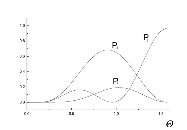
FIG. 1.: Angular dependence of the acoustic wave attenuation coefficients for various polarizations. These results are obtained for $T=1\,$K, $B=10\,$T, $1/M=60\,$K; consequently $\delta=3.0\,$K, $\eta_{l}=0.2$, $\eta_{t}=0.07\,$.

 

 

 

 

 

 

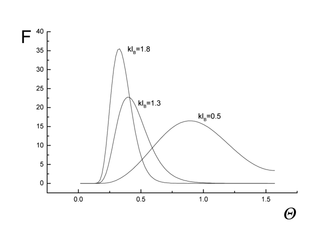
FIG. 2.: The inverse time (3.7) may be represented in the form $\tau_{l}^{-1}=L_{z}^{-1}\exp{[(\mu-\delta)/T]}\cdot$ $F(B,T,k,\theta)$. In this figure $F$ is calculated for $B=10\,$T, $T=1\,$K, $\mu-\delta=3\,$K.

REFERENCES

[1]
I. P. Eisenstein, A. C. Gossard, N. Naraynamurti, Phys. Rev. Lett. 59,
1341 (1987).
[2]
L. J. Challis, A. J. Kent, V. W. Rampton, Semicond. Sci. Technol. 5,
1179 (1990).
[3]
A. J. Kent, D. J. McKitterick, L. J. Challis, P. Hawker, C. J. Mellor,
and M. Henini , Phys. Rev. Lett. 69, 1684 (1992).
[4]
V. W. Rampton, K. McEnaney, A. G. Kozorezov, P. J. A. Carter, C. D. W.
Wilkinson, M. Henin, and O. H. Hugle, Semicond. Sci. Technol. 7, 641
(1992).
[5]
A. Wixforth, J. P. Kotthaus, and G. Weimann, Phys. Rev. Lett. 56, 2104
(1986).
[6]
A. Wixforth, J. Scriba, M. Wassermeier, J. P. Kotthaus, G. Weimann, and
W. Schlapp, Phys. Rev. B 40, 7874 (1989).
[7]
A. Esslinger, R. W. Winkler, C. Rocke, A. Wixforth, J. P. Kotthaus,
H. Nickel, W. Schlapp, and R. Lösch, Surface Sci. 305, 83 (1994).
[8]
R. L. Willett, M. A. Paalanen, R. R. Ruel, K. W. West, L. N. Pfeifer,
and D. J. Bishop, Phys. Rev. Lett. 65, 112 (1990).
[9]
R. L. Willett, Surface Sci. 305, 76 (1994).
[10]
S. V. Iordanskii, and B. A. Muzykantskii, Zh. Eksp. Teor. Fiz.96,
1783 (1989)
[JETP 69, 1006 (1989)].
[11]
S. Iordanskii, and Y. Levinson, Phys. Rev. B 53, 7308 (1996).
[12]
A. Knäbchen, Y. B. Levinson, and O. Entin-Wohlman, Phys. Rev. B 54,
10696 (1996).
[13]
O. Weis in Nonequilibrium Phonons in Nonmetallic Crystals ed. W.
Eisenmenger, and A. A. Kaplyanskii, P.1 (North-Holland, Amsterdam,
1986).
[14]
A. Bartels, T. Dekorsy, H. Kurz, and K. Köhler, Physica B 263-264, 45 (1999).
[15]
I. L. Aleiner, and B. I. Shklovskii, Int. J. of Mod. Phys. 8, 801
(1994).
[16]
S. L. Sondhi, A. Karlhede, S. A. Kivelson, and E. H. Rezayi, Phys.
Rev. B 47, 16419 (1993).
[17]
H. A. Fertig, L. Brey, R. Côté, and A. H. MacDonald ,
Phys. Rev. B 50, 11018 (1994).
[18]
L. Brey, H. A. Fertig, R. Côté, and A. H. MacDonald ,
Phys. Rev. Lett. 75, 2562 (1995).
[19]
S. E. Barret, G. Dabbagh, L. N. Pfeifer, K. W. West, and
R. Tycko, Phys. Rev. Lett. 74, 5112 (1995).
[20]
I. Kukushkin, K. v. Klitzing, and K. Eberl, Phys. Rev. B 60, 2554
(1999).
[21]
Yu. A. Bychkov, T. Maniv, and I. D. Vagner, Phys. Rev. B 53, 10148
(1996).
[22]
S. V. Iordanskii, Pis’ma Zh. Eksp. Teor. Fiz. 66, 428 (1997)
[JETP Lett. 66, 459 (1997)].
[23]
Yu. A. Bychkov, S. V. Iordanskii, and G. M. Éliashberg, Pis’ma Zh.
Eksp. Teor. Fiz. 33, 152 (1981)
[Sov. Phys. JETP Lett. 33, 143 (1981)].
[24]
C. Kallin, and B. I. Halperin, Phys. Rev. B 30, 5655 (1984).
[25]
I. V. Lerner, and Yu. E. Lozovik, Zh. Eksp. Teor. Fiz. 78, 1167
(1980)
[Sov. Phys. JETP 51, 588 (1980)].
[26]
S. M. Dickmann, and S. V. Iordanskii, Zh. Eksp. Teor. Fiz. 110, 238
(1996)
[JETP 83, 128 (1996)].
[27]
Yu. A. Bychkov, and E. I. Rashba, Zh. Eksp. Teor. Fiz. 85, 1826
(1983)
[Sov. Phys. JETP 58, 1062 (1983)].
[28]
We exclude from the consideration the effects of the heterostructure edges,
where the gain may be much larger than , and spatial charge
density fluctuations are possible.
[29]
A. B. Dzyubenko, and Yu. E. Lozovik, Fiz. Tverd. Tela (Leningrad) 26, 1540
(1984)
[Sov. Phys. Solid State 26, 938 (1984)].
[30]
M. Rasolt, B. I. Halperin, and D. Vanderbilt, Phys. Rev. Lett. 57, 126
(1986).
[31]
Yu. A. Bychkov, and S. V. Iordanskii, Fiz. Tverd. Tela (Leningrad)
29, 2442 (1987)
[Sov. Phys. Solid State 29, 1405 (1987)].
[32]
V. F. Gantmakher, and Y. B. Levinson, Carrier Scattaring in
Metals and Semiconductors (North-Holland, Amsterdam, 1987).
[33]
Yu. A. Bychkov, E. I. Rashba, Pis’ma Zh. Eksp. Teor. Fiz. 39, 66
(1984)
[Sov. Phys. JETP Lett. 39, 78 (1984)].
[34]
M. I. D’yakonov, and V. Yu. Kachorovskii, Fiz. Tekh. Poluprovodn.
20, 178 (1986)
[Sov. Phys. Semicond. 20, 110 (1986)].
[35]
Note that the screening does not occur in our system due to the absence of
free charges.
[36]
I. S. Gradshteyn, and I. M. Ryzhik, Table of Integrals, Series, and
Products (Academic Press, San Diego, 1994).
[37]
L. D. Landau, and E. M. Lifshitz, Theory of Elasticity (Pergamon
Press, Oxford, 1970).
[38]
D. G. Polyakov, and B. I. Shklovskii, Phys. Rev. B 48, 11167 (1993).
[39]
L. E. Golub, A. V. Scherbakov, and A. V. Akimov, J. Phys.: Condens. Matter
8, 2163 (1996).
[40]
A. V. Akimov, Physica B 263-264, 175 (1999).