The Effect of Shear on Phase-Ordering Dynamics with Order-Parameter-Dependent Mobility: The Large-n Limit

Abstract

The effect of shear on the ordering-kinetics of a conserved order-parameter system with $O(n)$ symmetry and order-parameter-dependent mobility $\Gamma({\,\vec{\phi}}\,)\propto(1-{\vec{\phi}}\,^{2}/n)^{\alpha}$ is studied analytically within the large-$n$ limit. In the late stage, the structure factor becomes anisotropic and exhibits multiscaling behavior with characteristic length scales $(t^{2\alpha+5}/\ln t)^{1/2(\alpha+2)}$ in the flow direction and $(t/\ln t)^{1/2(\alpha+2)}$ in directions perpendicular to the flow. As in the $\alpha=0$ case, the structure factor in the shear-flow plane has two parallel ridges.

I Introduction

The dynamics of the ordered phases when a system is quenched from the high temperature phase into the low temperature region of two- or more-ordered phases has been of intense interest[1]. It is now well established that in the late stage, both the equal time pair correlation function $C({\bf r},t)$ and the structure factor $S({\bf k},t)$ obtained by the Fourier transform of $C({\bf r},t)$ obeys standard scaling. By standard scaling it is meant that $C({\bf r},t)$ and $S({\bf k},t)$ can be written as $f(r/L)$ and $L^{d}g(kL)$ respectively, where $f(r/L)$ and $g(kL)$ are the scaling functions and $L(t)$ is the characteristic length scale in the system. For scaling to hold, $L(t)$ must be well separated from other length scales that may be present in the system. In most of the systems undergoing phase-ordering kinetics, the characteristic length scale $L(t)$ has a power-law dependence on the time $t$ elapsed since the quench, $L(t)\sim t^{1/z}$. The growth exponent $z$ depends on whether or not the order parameter is conserved. In the absence of shear, but with a constant mobility $\Gamma$, for nonconserved order parameter systems $z=2$ and for conserved order parameter with no hydrodynamic effects $z=3$ (for scalar fields) and 4 (for vector fields). The characteristic length scale $L(t)$ is normally associated with the wavevector $k_{m}$ at which the spherically symmetric structure factor $S({\bf k},t)$ is maximum (i.e. $k_{m}\sim L^{-1}$).

When the phase-separating system is subjected to uniform shear[2], the isotropy in the structure factor is broken as the domains grow faster in the flow direction than in directions perpendicular to the flow. This anisotropy is confirmed by simulation[3, 4, 5, 6] analytical[7], numerical[8] and experimental results[9, 10, 11]. We have previously shown analytically that within the large-$n$ limit[7], the structure factor exhibits multiscaling with characteristic lengths $k_{my}^{-1}=k_{mz}^{-1}\sim(t/\ln t)^{1/4}$ and $k_{mx}^{-1}\sim(t^{5}/\ln t)^{1/4}$ in directions perpendicular to the flow and parallel to the flow respectively. For the scalar case (without hydrodynamic effects), renormalization group arguments[6] predicts $k_{my}^{-1}\sim t^{1/3}$ and $k_{mx}^{-1}\sim t^{4/3}$, for the ’viscous hydrodynamic’ regime Läuger et al.[11] found experimentally $k_{my}^{-1}\sim t$ and $k_{mx}^{-1}\sim t^{2}$. The ratio $k_{mx}/k_{my}\sim 1/t$, is consistent with analytical, numerical, simulational and experimental results.

In the case of unsheared phase-separation, there has been much study of the effects of an order-parameter-dependent mobility[12, 13, 14, 15, 16, 17, 18]. It was suggested that a mobility of the form $\Gamma(\phi)=1-\phi^{2}$ is appropriate for deep quenches[12] and to account for the effects of external field such as gravity[13]. Simulational calculations[14] performed on phase-separation with scalar order parameter and mobility $\Gamma(\phi)=1-a\phi^{2}$, show that for $a=1$, $z=4$ instead of 3 which is a result for constant mobility. A crossover from $z=4$ to 3 was found for the case where $a<1$ (with $a>0$)[14]. For an $n$-vector order parameter, the simulation results[15] done with $\Gamma(\,{\vec{\phi}}\,)=1-a{\vec{\phi}}\,^{2}/n$ for $n=2$, 3 and 4, shows a crossover from $z=6$ to $z=4$ for $a<1$, while for $a=1$, $z=6$. Emmott et al. [16, 17] considered a more general expression for the mobility given by

$$\Gamma(\,{\vec{\phi}}\,)=\Gamma_{0}\,(1-{\vec{\phi}}\,^{2}/n)^{\alpha}\,,$$ (1)

where $\alpha\in\Re^{+}$. For scalar fields[16] in the Lifshitz-Slyozov limit, they found $z=3+\alpha$ while for conserved vector fields within the large-$n$ limit[17], multiscaling was found with two length scales $t^{1/2(\alpha+2)}$ and ${k_{m}}^{-1}\sim(t/\ln t)^{1/2(\alpha+2)}$. A different form for the mobility, $\Gamma(\phi)=1/(1+\exp(\,\alpha\phi-\beta\phi^{2})\,)$, where both $\alpha$ and $\beta$ are positive (with $\beta>\alpha$) was used by Ahluwalia[18] in simulating the Cahn-Hilliard model of phase-separation. The domain patterns were found to be similar to the ones observed in viscoelastic phase separation. It is clear that different forms of mobility can be used depending on the type of problem concerned.

In this paper we are mainly concerned with the dynamics of the large-$n$ conserved order parameter with the simplest shear flow following a quench from the high temperature phase to zero temperature, and the case with an order-parameter-dependent mobility given by (1). We show that in the late stage, the structure factor becomes anisotropic and shows multiscaling behavior[19] (i.e. $S({\bf k},t)\sim(\,(L_{x}L_{y}L_{z})^{\varphi(k_{x}L_{x},k_{y}L_{y},k_{z}L_{z})}\,)$ with characteristic length scales $L_{x}\sim k_{mx}^{-1}\sim(t^{2\alpha+5}/\ln t)^{1/2(\alpha+2)}$, $L_{y}\sim k_{my}^{-1}\sim(t/\ln t)^{1/2(\alpha+2)}$, and $L_{z}\sim k_{mz}^{-1}\sim(t/\ln t)^{1/2(\alpha+2)}$ extracted from the maxima of the structure factor. In the $k_{z}=0$ plane, there are two parallel ridges, whose height and length depends on $\alpha$. These parallel ridges have been observed in experiments[9] for scalar fields in the absence of shear with $\alpha=0$. It is worth mentioning that multiscaling is believed to be an artifact of the large-$n$ approximation as in the case of constant mobility and zero shear[20]. For systems with finite $n$, we expect scaling to be recovered asymptotically, although multiscaling may be exhibited as a preasymptotic effect[21].

The paper is organised as follows: In the next section, model equations which take into the account both shear and non constant mobility are introduced. In section III, an exact solution for the structure factor is obtained in the scaling limit. The discussion of the results for specific values of $\alpha$ (i.e $\alpha=1$ and 2) are presented in section IV. Concluding remarks are given in section V.

II Model Equations

In order to study the phase-separating system, the Cahn-Hilliard equation (generalised to $n$-vector order parameter ${\vec{\phi}}$) is given by

$$\partial_{t}{\vec{\phi}}=-{\bf\nabla}\cdot\left[\,\Gamma({\vec{\phi}}){\bf\nabla}\left(-{\bf\nabla}^{2}{\vec{\phi}}+{\vec{\phi}}-({\vec{\phi}}\,^{2}/n)\,{\vec{\phi}}\,\right)\right].$$ (2)

We are interested in a system with uniform shear flow which has a velocity field of the form ${\bf v}=\gamma y\,{\bf e_{x}}$, where $\gamma$ is the constant shear rate and ${\bf e_{x}}$ is a unit vector in the flow direction. For an incompressible system in the presence of shear, the term $({\bf v}\cdot{\bf\nabla}){\vec{\phi}}$ is added on the left hand side of (2) leading to

$$\partial_{t}{\vec{\phi}}+\gamma y\partial_{x}{\vec{\phi}}=-{\bf\nabla}\cdot\left[\Gamma({\vec{\phi}}){\bf\nabla}\left(-{\bf\nabla}\,^{2}{\vec{\phi}}+{\vec{\phi}}-({\vec{\phi}}\,^{2}/n){\vec{\phi}}\,\right)\right].$$ (3)

In the limit $n\rightarrow\infty$, ${\vec{\phi}}^{2}/n$ is replaced by its average in the usual way, and eq.(3) reduces to a linear self-consistent equation whose Fourier transform is given by

$$\frac{\partial\phi_{\bf k}}{\partial t}-\gamma k_{x}\frac{\partial\phi_{\bf k}}{\partial k_{y}}=-{\bf k^{2}}a(t)^{\alpha}\,[{\bf k^{2}}-a(t)]\,\phi_{\bf k},$$ (4)

where $\Gamma_{0}$ has been absorbed into the time scale, $\phi$ is (any) one component of $\vec{\phi}$, and $a(t)=1-\langle\phi^{2}\rangle$. Eq.(4) has recently been solved numerically within a ’self-consistent one-loop’ approximation for a scalar order parameter in two dimensions by Gonnella et al.[22]. We believe that the oscillations (whose amplitudes decreases quite rapidly as $\alpha$ increases) found in[22] are slowly-decaying preasymptotic transients.

III Exact Solution in the Scaling Limit

Eq.(4) is a first order linear partial differential equation which can be easily solved by change of variables: $(k_{x},k_{y},t)\rightarrow(k_{x},\sigma,\tau)$, with $t=\tau$ and $\sigma=k_{y}+\alpha k_{x}\tau$. With this transformation the left hand side of (4) becomes $\partial\phi_{k}/\partial\tau$, and straight forward integration gives (after transforming back to original variables) $\phi_{\bf k}(t)=\phi_{\bf k}(0)\exp f({\bf k},t)$, where

$$f({\bf k},t) = -(\kappa^{2}+\mu^{2})^{2}\,b_{0}(t)+4\gamma k_{x}\mu\,(\kappa^{2}+\mu^{2})\,b_{1}(t)$$ (8)

$$-2\gamma^{2}k_{x}^{2}\,(\kappa^{2}+3\mu^{2})\,b_{2}(t)+4\gamma^{3}k_{x}^{3}\,\mu\,b_{3}(t)$$

$$-\gamma^{4}k_{x}^{4}\,b_{4}(t)+(\kappa^{2}+\mu^{2})\,p_{0}(t)-2\gamma k_{x}\mu\,p_{1}(t)$$

$$+\gamma^{2}k_{x}^{2}\,p_{2}(t),$$

with $\kappa^{2}=k_{x}^{2}+k_{z}^{2}$, $\mu=k_{y}+\gamma k_{x}t$, $b_{m}(t)=\int_{0}^{t}dt^{\prime}\,t^{\prime m}\,a(t^{\prime})^{\alpha}$, $p_{m}(t)=\int_{0}^{t}dt^{\prime}\,t^{\prime m}\,a(t^{\prime})^{\alpha+1}$.

From dimensional analysis, it is easy to see that to leading order in $t$: $a(t)\sim t^{-1/(\alpha+2)}$, $L_{y}\sim L_{z}\sim t^{1/2(\alpha+2)}$ and $L_{x}\sim t^{(2\alpha+5)/2(\alpha+2)}$, with the dominant part of the $k_{x}$-dependence coming from the shear terms. In fact there are logarithmic corrections to these power law relations as we will see. It is reasonable to make the ansatz $a(t)\sim(\ln t/t)^{1/(\alpha+2)}$ ( this is true for $\gamma=0$[17] ) in the large-$t$ limit. Then to leading order in $t$, we have

$$b_{m}(t) = \frac{2\,t^{m}\,b_{0}(t)}{m\alpha+2m+2}\,,$$ (9)

$$p_{m}(t) = \frac{t^{m}\,p_{0}(t)}{m\alpha+2m+1}\,.$$ (10)

Substituting (10) in eq. (8) after making the following change of variables,

$$\gamma k_{x}=\sqrt{\frac{p_{0}(t)}{t^{2}b_{0}(t)}}\,u\,,\,\,\,k_{y}=\sqrt{\frac{p_{0}(t)}{b_{0}(t)}}\,v\,,\,\,\,k_{z}=\sqrt{\frac{p_{0}(t)}{b_{0}(t)}}\,w\,,$$ (11)

the structure factor $S({\bf k},t)=\langle\phi_{\bf k}(t)\phi_{-\bf k}(t)\rangle$ becomes

$$S({\bf k},t) = \Delta\exp\left(2\,\frac{p_{0}^{2}}{b_{0}}F(u,v,w)\right)\,,$$ (12)

$$F(u,v,w) = -\frac{u^{4}}{5}A_{0}(\alpha)-u^{3}vA_{1}(\alpha)-2u^{2}v^{2}A_{2}(\alpha)$$ (16)

$$-2uv^{3}A_{3}(\alpha)-v^{4}+\frac{8}{15}u^{2}A_{5}(\alpha)$$

$$+\frac{4}{3}uvA_{4}(\alpha)+v^{2}+w^{2}-w^{4}-2v^{2}w^{2}$$

$$-\frac{2}{3}u^{2}w^{2}A_{2}(\alpha)-2uvw^{2}A_{3}(\alpha)\,,$$

where contributions to $F$ which vanish as $t\rightarrow\infty$ (at fixed $u,v,w$) have been dropped, $\Delta$ is the size of the initial fluctuation, $\langle\phi_{i}({\bf r},0)\phi_{j}({\bf r^{\prime}},0)\rangle=\Delta\delta_{ij}\delta({\bf r-r^{\prime}})$, and

$$A_{0} = 5-\frac{40}{\alpha+4}+\frac{60}{2\alpha+6}-\frac{40}{3\alpha+8}+\frac{10}{4\alpha+10}\,,$$ (17)

$$A_{1} = 4-\frac{24}{\alpha+4}+\frac{24}{2\alpha+6}-\frac{8}{3\alpha+8}\,,$$ (18)

$$A_{2} = 3-\frac{12}{\alpha+4}+\frac{6}{2\alpha+6}\,,$$ (19)

$$A_{3} = 2-\frac{4}{\alpha+4}\,,$$ (20)

$$A_{4} = \frac{3}{2}-\frac{3}{2\alpha+6}\,,$$ (21)

$$A_{5} = \frac{15}{8}-\frac{30}{8\alpha+24}+\frac{15}{16\alpha+40}\,,$$ (22)

with $A_{m}(\alpha=0)=1$. In order to find the exact form of $b_{0}$ and $p_{0}$ in the large-$t$ limit, we consider the self-consistent equation for $a(t)$ given by

$$a(t) = 1-\int\frac{d^{3}k}{(2\pi)^{3}}\,S({\bf k},t)$$ (23)

$$= 1-\frac{\Delta}{(2\pi)^{3}\gamma t}\left(\frac{p_{0}}{b_{0}}\right)^{3/2}$$ (25)

$$\times\int du\,dv\,dw\,\exp\left(2\,\frac{p_{0}^{2}}{b_{0}}\,F(u,v,w)\right).$$

The above integral can easily be evaluated by the method of steepest descent using the points of global maxima in $F(u,v,w)$ provided $p_{0}^{2}/b_{0}\rightarrow\infty$ as $t\rightarrow\infty$ ( this is the case we assumed before), therefore eq.(25) becomes

$$1=\frac{C_{1}(\alpha)\Delta}{\gamma tp_{0}^{3/2}}\exp\left(2\,\frac{p_{0}^{2}}{b_{0}}\,F_{m}(\alpha)\right)$$ (26)

where $C_{1}(\alpha)$ is a constant, $F_{m}(\alpha)$ is the value at the maxima $(\,u_{m}(\alpha),v_{m}(\alpha),w_{m}(\alpha)\,)$. The assumption that $a(t)\ll 1$ for $t\gg 1$ has also been used.

$\alpha=1$
Position (u,v,w)	Number	F	Value	Type (3D)	Type (2D)
$(0,0,0)$	1	0	0	Min	Min
$\pm(\sqrt{55/6}/3,0,0)$	2	55/168	.32738	IS	IMax
$\pm((33-\sqrt{165})/18\sqrt{2},-1/\sqrt{2},0)$	2	$31/168-\sqrt{55/3}/28$	.03160	S2	S
$\pm((33+\sqrt{165})/18\sqrt{2},-1/\sqrt{2},0)$	2	$31/168+\sqrt{55/3}/28$	.33744	S1	Max
$\pm(0,0,1/\sqrt{2})$	2	1/4	.25	S1	-
$\pm(\sqrt{22}/3,-\sqrt{11/2}/4,\pm\sqrt{5/2}/4)$	4	39/112	.34821	Max	-
$\alpha=2$
Position (u,v,w)	Number	F	Value	Type ($3D$)	Type $(2D)$
$(0,0,0)$	1	0	0	Min	Min
$\pm(\sqrt{7/8},0,0)$	2	14/45	.31111	IS	IMax
$\pm((7-\sqrt{7})/4\sqrt{2},-1/\sqrt{2},0)$	2	$31/180-\sqrt{7}/18$	.02524	S2	S
$\pm((7+\sqrt{7})/4\sqrt{2},-1/\sqrt{2},0)$	2	$31/180+\sqrt{7}/18$	.31921	S1	Max
$\pm(0,0,1/\sqrt{2})$	2	1/4	.25	S1	-
$\pm(\sqrt{35}/4,-\sqrt{7/5}/2,\pm\sqrt{3/5}/2)$	4	59/180	.32778	Max	-

Table 1. Stationary points of $F(u,v,w)$: Max = maximum, Min = minimum, S = saddle point (2D), S$n$ = saddle point of type $n$ (the matrix of second derivatives has $n$ positive eigenvalues), IS = ‘inflection saddle point’ (one positive, one zero, one negative eigenvalue), IMax = ‘inflection maximum’ (one zero, one negative eigenvalue). See also FIG. 1. for $2D$ results.

Therefore to leading logarithmic accuracy, (26) leads to

$$p_{0}^{2}(t) \approx \frac{b_{0}\ln t}{2F_{m}}+\frac{3b_{0}\ln b_{0}}{8F_{m}}\,,$$ (27)

$$2\,p_{0}\,\frac{dp_{0}}{dt} \approx \frac{db_{0}}{dt}\left[\frac{\ln t}{2F_{m}}+\frac{3\ln b_{0}}{8F_{m}}\right].$$ (29)

Using (29) and the relations $db_{0}/dt=a^{\alpha}$, $dp_{0}/dt=a^{\alpha+1}$ we get

$$a(t)\approx\left(\frac{\ln b_{0}}{b_{0}}\right)^{1/2}\left[\frac{\ln t}{8F_{m}\ln b_{0}}+\frac{3}{32F_{m}}\right]^{1/2},$$ (30)

from which $b_{0}$ (since $db_{0}/dt=a^{\alpha}$) is found to be

$$b_{0}(t) \approx \left(\frac{\alpha+2}{2}t\right)^{2/(\alpha+2)}$$ (32)

$$\times\left(\frac{2\ln t}{\alpha+2}\left[\frac{\alpha+2}{16F_{m}}+\frac{3}{32F_{m}}\right]\right)^{\alpha/(\alpha+2)},$$

whence,

$$\frac{p_{0}^{2}(t)}{b_{0}(t)} \approx \frac{\ln t}{2F_{m}}\left[1+\frac{3}{2(\alpha+2)}\right]\,,$$ (33)

$$a(t) \approx \left(\frac{4}{(\alpha+2)^{2}}\frac{\ln t}{t}\right)^{1/(\alpha+2)}$$ (36)

$$\times\left[\frac{\alpha+2}{16F_{m}}+\frac{3}{32F_{m}}\right]^{1/(\alpha+2)}\,.$$

The above results for $a(t)$, $b_{0}(t)$ and $p_{0}(t)$ justify our original ansatz. From (11) we can define the characteristic length scales in three directions: $L_{x}=\gamma(t^{2}b_{0}/p_{0})^{1/2}\sim\Upsilon(\alpha)\,\gamma\,(t^{2\alpha+5}/\ln t)^{1/2(\alpha+2)}$, and $L_{y}=L_{z}=(b_{0}/p_{0})^{1/2}\sim\Upsilon(\alpha)\,(t/\ln t)^{1/2(\alpha+2)}$, by setting $u=k_{x}L_{x}$, $v=k_{y}L_{y}$, and $w=k_{z}L_{z}$, where

$$\Upsilon^{-1}(\alpha)=\sqrt{2}\left(\frac{4}{(\alpha+2)^{2}}\left[\frac{\alpha+2}{16F_{m}}+\frac{3}{32F_{m}}\right]\right)^{1/2(\alpha+2)}\,.$$ (37)

Exact values for $F_{m}(\alpha)$ and $(\,u_{m}(\alpha),v_{m}(\alpha),w_{m}(\alpha)\,)$ can be found by specifying values of $\alpha$. For example, values for $\alpha=1$ and 2 are shown in table 1, while for $\alpha=0$, results presented in[7] are recovered.

Using (16), (26), and (36), it is easy to show that the structure factor becomes

$$S({\bf k},t)={\rm Const.}\,\left[\ln V_{s}\right]^{3/2}V_{s}^{F({\bf q})/F_{m}}\,,$$ (38)

with scaled momentum ${\bf q}$ and ’scale volume’ $V_{s}$ given by

$${\bf q} = (k_{x}L_{x},k_{y}L_{y},k_{z}L_{z})\,,$$ (39)

$$V_{s} = L_{x}L_{y}L_{z}\sim\gamma t^{(7+2\alpha)/2(\alpha+2)}/(\ln t)^{3/2(\alpha+2)}\,,$$ (40)

respectively. Eq.(38) exhibits multiscaling behavior (i.e the power of the ’scale volume’ depends continuously on the scaling variables). We anticipate, however, that for finite $n$, standard scaling will be recovered and the $\ln t$ terms (which appear in the characteristic length scales) will be absent as has been shown explicitly for the case with both $\alpha$ and $\gamma$ = 0[20].

IV Results

Both the positions of the stationary points of $F(u,v,w)$ and its value depend on $\alpha$ ( apart from points (0,0,0) and $\pm(0,0,1/\sqrt{2})$ ), see table 1. The global picture of $S({\bf k},t)$ is determined by $F(u,v,w)$ (i.e. the stationary points and their type together with values of $F(u,v,w)$ at stationary points) because $\ln S({\bf k},t)=(F(u,v,w)/F_{m})\ln V_{s}$ [plus $\bf k$-independent terms]. The features of $F(u,v,w)$ for $\alpha=1$ and 2 are summarised in table 1 and table 2.

The parallel ridges found in Figure 1 are similar to ones found in experiments[9]. The global maxima are connected by almost straight ridges to the ’inflexion maxima’. As the value of $\alpha$ increases, the height of each ridge decreases towards the limiting value $F=1/4$ (and also the length of each ridge increases) while the line connecting the two saddle points and the minimum approaches the line $u=-v$ with $F=0$. In the $(k_{x},k_{y})$ plane, the ridges become narrower, higher, and closer together as a function of $\bf k$ with increasing time $t$. The angle $\theta$ between the ridges and the shear direction ($k_{y}$ direction in this case) is a good measure of theory against experiments because the depth of the temperature quench is unimportant as far as the time dependence is concerned. We find

$$\tan(\theta)=\frac{C_{2}(\alpha)}{\gamma t}\,,$$ (41)

where $C_{2}(\alpha)$ is a constant which depends on $\alpha$, e.g. $C_{2}(0)=2(1-1/\sqrt{6}),C_{2}(2)=(7-\sqrt{7})/4$. Eq. (41) implies that in the $(k_{x},k_{y})$ plane, the ridges move closer to the shear direction as time increases, this behavior is found both in simulations[6] and experiments[11].

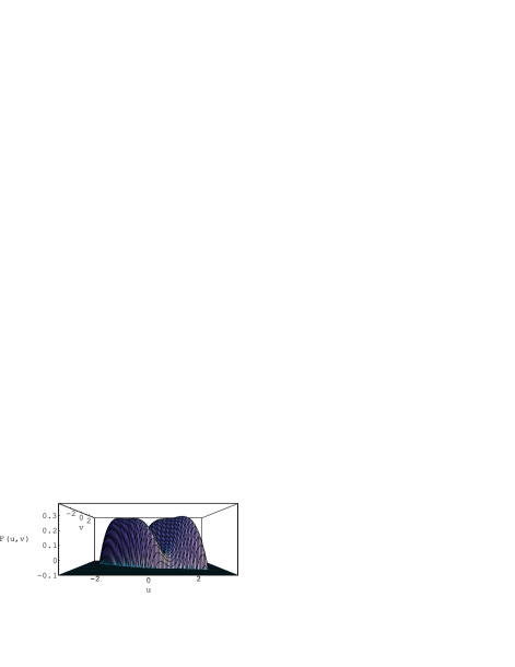
FIG. 1.: The graph of $F(u,v,0)$ for $\alpha=1$. Values for $F(u,v,0)<-0.1$ are not shown.

In the $(u,w)$ plane, there are four maxima, four saddle points and the global minimum at the origin. These are shown in table 2 (for $\alpha=1,2$), and they can easily be seen in Figure 2 for $\alpha=1$. When $\alpha$ increases, the peaks and the higher saddle point (i.e saddle point with higher value of $F(u,0,w)$ reduces towards the limiting value $F=1/4$ (i.e $F_{m}(u,0,w)$ is deformed towards a ring of radius $1/\sqrt{2}$). For each value of $\alpha$, the structure factor pattern in the $(k_{x},k_{z})$ plane will decrease faster in the flow (i.e $k_{x}$) direction as a function of $t$, resulting in an elliptical shape with major axis along $k_{z}$ direction. This elliptical shape has been observed in experiments[11] for scalar fields while the four peaks were not observed.

The excess viscosity $\Delta\eta$, and normal stresses $\Delta N_{1}$, $\Delta N_{2}$ derived by Onuki[2] can be evaluated in the asymptotic limit:

$$\Delta\eta = -(1/\gamma)\int\,\frac{d^{3}k}{2\pi)^{3}}\,k_{x}k_{y}\,S({\bf k},t)\,,$$ (42)

$$\sim \frac{1}{\gamma^{2}}\,\left(\frac{\ln t}{t^{\alpha+3}}\right)^{1/(\alpha+2)}\,,$$ (43)

$$\Delta N_{1} = \int\,\frac{d^{3}k}{2\pi)^{3}}\,(k_{y}^{2}-k_{x}^{2})\,S({\bf k},t)\,,$$ (44)

$$\sim \left(\frac{\ln t}{t}\right)^{1/(\alpha+2)}\,,$$ (45)

$$\Delta N_{2} = \int\,\frac{d^{3}k}{2\pi)^{3}}\,(k_{y}^{2}-k_{z}^{2})\,S({\bf k},t)\,,$$ (46)

$$\sim \left(\frac{\ln t}{t}\right)^{1/(\alpha+2)}\,.$$ (47)

Numerical calculations[22] show that both excess viscosity $\Delta\eta(t)$, and the normal stress $\Delta N_{1}(t)$ reach a peak before the asymptotic scaling result. It is not possible to realise this effect as our calculations are strictly valid in the asymptotic regime.

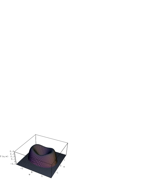
FIG. 2.: The graph of $F(u,0,w)$ for $\alpha=1$. Values for $F(u,0,w)<-0.1$ are not shown.

$\alpha=1$
Position (u,w)	No.	F	Value	Type
$(0,0)$	1	0	0	Min
$\pm(\sqrt{55/6}/3,0)$	2	55/168	.32738	S
$\pm(0,1/\sqrt{2})$	2	1/4	.25	S
$\pm(\sqrt{110/129},\pm\sqrt{5/43})$	4	100/301	0.3322	Max
$\alpha=2$
Position (u,w)	No.	F	Value	Type
$(0,0)$	1	0	0	Min
$\pm(\sqrt{7/2}/2,0)$	2	14/45	.31111	S
$\pm(0,1/\sqrt{2})$	2	1/4	.25	S
$\pm(\sqrt{35/3}/4,\pm 1/3)$	4	17/54	0.31481	Max

Table 2. Stationary points of $F(u,0,w)$: Max = maximum, Min = minimum, S = saddle point. See also FIG. 2.

In analogy to 2-$D$ numerical calculations presented in[22], it is easy to repeat the calculation for 2-$D$ in the shear-flow ($k_{x}$ , $k_{y}$) plane. The self-consistent equation for $a(t)$ leads to (with $C_{3}(\alpha)$ constant)

$$1=\frac{C_{3}(\alpha)\Delta}{\gamma tp_{0}}\exp\left(2\,\frac{p_{0}^{2}}{b_{0}}\,F^{2D}_{m}(\alpha)\right)\,,$$ (49)

from which to leading order in $t$,

$$b_{0}(t) \approx \left(\frac{\alpha+2}{2}t\right)^{2/(2+\alpha)}$$ (51)

$$\times\left(\frac{2\ln t}{\alpha+2}\left[\frac{\alpha+2}{16F^{2D}_{m}}+\frac{1}{16F^{2D}_{m}}\right]\right)^{\alpha/(\alpha+2)}\,,$$

$$\frac{p_{0}^{2}(t)}{b_{0}(t)} \approx \frac{\ln t}{2F^{2D}_{m}}\left[1+\frac{1}{(\alpha+2)}\right]\,,$$ (53)

$$a(t) \approx \left(\frac{4}{(\alpha+2)^{2}}\frac{\ln t}{t}\right)^{1/(2+\alpha)}$$ (56)

$$\times\left[\frac{\alpha+2}{16F^{2D}_{m}}+\frac{1}{16F^{2D}_{m}}\right]^{1/(\alpha+2)}\,.$$

Using both (49) and (56), the structure factor can be written down as $S({\bf k},t)={\rm Const}.\,(\ln A_{s})A_{s}^{F({\bf q})/F^{2D}_{m}}$, where $A_{s}=L_{x}L_{y}$ is the ’scale area’ and ${\bf q}=(k_{x}L_{x},k_{y}L_{y})$ with $L_{x}\sim\gamma(t^{5+2\alpha}/\ln t)^{1/2(\alpha+2)}$, $L_{y}\sim(t/\ln t)^{1/2(\alpha+2)}$ and ${F}^{2D}=F(u,v,0)$. Therefore the structure factor pattern is similar to Figure 1. The oscillations between the peaks[22] which terminate the two parallel ridges, we believe are suppressed in the long time regime (i.e. they are the preasymptotic decaying transients).

V Summary and Remarks

We have analytically studied the effect of both shear and order-parameter-dependent mobility on phase-separation within the large-$n$ limit. Shear introduces anisotropy in the structure factor pattern because of different growth rates in the flow direction and directions perpendicular to flow. At fixed time $t$ and ${\bf k}$, $\alpha$ distorts the shape of the structure factor $S({\bf k},t)$ (this is evident in the $F(u,v,0)$ and $F(u,0,w)$ patterns). Similar to all studies previously done, the order-parameter-dependent mobility slows down the rate of coarsening (i.e. $L_{i}(\alpha=0)>L_{i}(\alpha\neq 0)$, where $i=x$, $y$, $z$). We believe the multiscaling found here to be the result of the large-$n$ approximation, and that for any finite $n$, standard scaling will be obtained with the same characteristic length scales but without the $\ln t$ terms, $L_{x}\sim t^{(2\alpha+5)/2(\alpha+2)}$, $L_{y}\sim t^{1/2(\alpha+2)}$, and $L_{z}\sim t^{1/2(\alpha+2)}$. The excess viscosity $\Delta\eta(t)$, and the normal stresses (i.e $\Delta N_{1}(t)$ and $\Delta N_{2}(t)$) relax to zero as $(\ln t/t^{\alpha+3})^{1/(\alpha+2)}$ and $(\ln t/t^{1/(\alpha+2)}$ respectively in the scaling limit. Again we expect logarithmic terms to be absent for finite $n$.

ACKNOWLEDGEMENTS

NR thanks A. Bray for suggesting this problem, and for discussions. This work was supported by the Commonwealth Scholarship Commission.

REFERENCES

• [1] A. J. Bray, Adv.ย Phys.ย 43, 357 (1994).
• [2] A. Onuki, J. Phys.: Condens. Matter 9, 6119 (1997), and references therein.
• [3] D. H. Rothman, Phys.ย Rev.ย Lett.ย 65, 3305 (1990).
• [4] P. Padilla and S. Toxvaerd, J. Chem.ย Phys.ย 106, 2342 (1997).
• [5] A. J. Wagner and J. M. Yeomans, preprint (cond-mat/9904033).
• [6] F.Corberi, G. Gonnella, and A. Lamura, preprint (cond-mat/9904423).
• [7] N. P. Rapapa and A. J. Bray, preprint (cond-mat/9904396).
• [8] F. Corberi, G. Gonnella, and A. Lamura, Phys.ย Rev.ย Lett.ย 81, 3852 (1998).
• [9] C. K. Chan, F. Perrot, and D. Beysens, Phys.ย Rev.ย A 43, 1826 (1991).
• [10] T. Hashimoto, K. Matsuzaka, E. Moses, and A. Onuki, Phys.ย Rev.ย Lett.ย 74, 126 (1995).
• [11] J. Lรคuger, C. Laubner, and W. Gronski, Phys.ย Rev.ย Lett.ย 75, 3576 (1995).
• [12] J. S. Langer, M. Bar-on, and H. D. Miller, Phys.ย Rev. A,ย 11, 1417 (1975); K. Kitahara and M. Imada, Prog.ย Theor.ย Phys.ย Suppl.ย 64, 65 (1978).
• [13] D. Jasnow, in Far from Equilibrium Phase Transitions ed. L. Garrido ( Springer-Verlag, Berlin, 1988); K. Kitahara, Y. Oono, and D. Jasnow, Mod.ย Phys.ย Lett.ย Bย 2, 765 (1988).
• [14] S. Puri, A. J. Bray, and J. L. Lebowitz, Phys.ย Rev.ย Eย 56, 758 (1997); A. M. Lacasta, A. Hernandez-Machado, and J. M. Sacho, Phys.ย Rev.ย Bย 45, 5276 (1992).
• [15] F. Corberi and C. Castellano, Phys.ย Rev.ย Eย 58,4658 (1998).
• [16] A. J. Bray and C. L. Emmott, Phys.ย Rev.ย Bย 52, R685 (1995).
• [17] C. L. Emmott and A. J. Bray, Phys.ย Rev.ย Eย 59, 213 (1999).
• [18] R. Ahluwalia, Phys.ย Rev.ย Eย 59, 263 (1999).
• [19] A. Coniglio and M. Zannetti, Europhys.ย Lett.ย 10, 575 (1989).
• [20] A. J. Bray and K. Humayun, Phys.ย Rev.ย Lett.ย 68, 1559 (1992).
• [21] A. Coniglio, P. Ruggiero, and M. Zannetti Phys.ย Rev.ย Eย 50, 1046 (1994); F. Corberi, A. Coniglio, and M. Zannetti, Phys.ย Rev.ย E 51, 5469 (1995); C. Castellano and M. Zannetti, Phys.ย Rev.ย Lett.ย 77, 2742 (1996); Phys.ย Rev.ย E 53, 1430 (1996); Phys.ย Rev.ย E 58, 5410 (1998).
• [22] G.Gonnella, A. Lamura, and D. Suppa, preprint (cond-mat/9904422).