Topological Defects in
Nematic Droplets of Hard Spherocylinders

Abstract

Using computer simulations we investigate the microscopic structure of the singular director field within a nematic droplet. As a theoretical model for nematic liquid crystals we take hard spherocylinders. To induce an overall topological charge, the particles are either confined to a two-dimensional circular cavity with homeotropic boundary or to the surface of a three-dimensional sphere. Both systems exhibit half-integer topological point defects. The isotropic defect core has a radius of the order of one particle length and is surrounded by free-standing density oscillations. The effective interaction between two defects is investigated. All results should be experimentally observable in thin sheets of colloidal liquid crystals.

PACS: 61.30.Jf, 83.70.Jr, 77.84.Nh

I Introduction

Liquid crystals (LC) show behavior intermediate between liquid and solid. The coupling between orientational and positional degrees of freedom leads to a large variety of mesophases. The microscopic origin lies in anisotropic particle shapes and anisotropic interactions between the particles that constitute the material. The simplest, most liquid-like LC phase is the nematic phase where the particles are aligned along a preferred direction while their spatial positions are, like in an ordinary liquid, homogeneously distributed in space. The preferred direction, called the nematic director, can be macroscopically observed by illuminating a nematic sample between crossed polarizers.

There are many different systems that possess a nematic phase. Basically, one can distinguish between molecular LCs where the constituents are molecules and colloidal LCs containing mesoscopic particles, e.g., suspensions of tobacco mosaic viruses [1]. Furthermore there is the possibility of self-assembling rodlike micelles [2], that can be studied with small-angle neutron scattering [3].

There are various theoretical approaches to deal with nematic liquid crystals. On a coarse-grained level one may use Ginzburg-Landau theories, including phenomenological elastic constants. The central idea is to minimize an appropriate Frank elastic energy with respect to the nematic director field [4]. Second, there are spin models, like the Lebwohl-Lasher model, see, e.g., Refs. [5, 6, 7]. There the basic degrees of freedom are rotators sitting on the sites of a lattice and interacting with their neighbors. The task is to sample appropriately the configuration space. The third class of models consists of particles with orientational and positional degrees of freedom. Usually, the interaction between particles is modelled by an anisotropic pair potential. Examples are Gay-Berne particles, e.g. [8, 9] and hard bodies, e.g., hard spherocylinders (HSC) [10]. Beginning with the classical isotropic-nematic phase transition for the limit of thin, long needles due to Onsager [11], our knowledge has grown enormously for the system of hard spherocylinders. The bulk properties have recently been understood up to close packing. The phase diagram has been calculated by computer simulations [12], density-functional theory [13] and cell theory [14]. There are various stable crystal phases, like an elongated face-centered cubic lattice with ABC stacking sequence, a plastic crystal, smectic-A phase, nematic and isotropic fluid. Besides bulk properties, one has investigated various situations of external confinement, like nematics confined to a cylindrical cavity [15] or between parallel plates [16, 17]. Also effects induced by a single wall have been studied, like depletion-driven adsorption [18], anchoring [19], wetting [20], and the influence of curvature[21]. Furthermore, solid bodies immersed in nematic phases experience non-trivial forces [22, 23, 24], and point defects experience an interaction [25].

Topological defects within ordered media are deviations from ideal order, loosely speaking, that can be felt at an arbitrary large separation distance from the defect position. Complicated examples are screw dislocations in crystalline lattices and inclusions in smectic films [26]. To deal with topological defects the mathematical tools of homotopy theory may be employed [27] to classify all possible structures. The basic ingredients are the topology of both the embedding physical space and the order parameter space. For the case of nematics, there are two kinds of stable topological defects in 3d, namely point defects and line defects, whereas in 2d there are only point defects. These defects arise when the system is quenched from the isotropic to the nematic state [28]. Also the dynamics have been investigated [29] experimentally. On the theoretical side, there is the important work within the framework of Landau theory by Schopohl and Sluckin on the defect core structure of half-integer wedge disclinations [30] and on the hedgehog structure [31] in nematic and magnetic systems. The latter predictions have been confirmed with computer simulations of lattice spin models [32]. The topological theory of defects has been used to prove that a uniaxial nematic either melts or exhibits a complex biaxial structure [33]. Sonnet, Kilian and Hess [34] have considered droplet and capillary geometries using an alignment tensor description.

The investigation of equilibrium topological defects in nematics has received a boost through a striking possibility to stabilize defects by imprisoning the nematic phase within a spherical droplet. The droplet boundary induces a non-trivial effect on the global structure within the droplet. Moreover, it can be experimentally controlled in a variety of ways to yield different well-defined boundary conditions, namely homeotropic or tangential ones. One famous experimental system are polymer-dispersed LCs. Concerning nematic droplets, there are various studies using the Lebwohl-Lasher model [5, 6, 7]. There are investigations of the droplet shape [35, 36], the influence of an external field [37], and chiral nematic droplets [38], structure factor [39], and ray propagation [40]. Also simulations of Gay-Berne droplets have been performed [41]. Other systems that exhibit topological defects are nematic emulsions [42, 43, 44], and defect gels in cholesteric LCs [45]. The formation of disclination lines near a free nematic interface was reported [46].

In this work we are concerned with the microscopic structure of topological defects in nematics. We use a model for rod-like particles with a pair-wise hard core interaction, namely hard spherocylinders. It accounts for both, the orientational degrees of freedom as well as the positional degrees of freedom of the particles constituting the nematic. Especially, it allows for mobility of the defect positions. This system is investigated with Monte Carlo computer simulations. There exist successful simulations of topological line defects using hard particles, namely integer [47] and half-integer line defects [48].

Here, we undertake a detailed study of the microscopic structure of the defect cores focusing on the behavior of the local nematic order and on the density field, an important quantity that has not been studied in the literature yet. As a theoretical prediction, we find that the arising half-integer point defects are surrounded by an oscillating density inhomogeneity. This can be verified in experiments. We also investigate the statistical properties of two defects interacting with each other extracting the distribution functions of the positions of the defect cores and their orientations. These are not accessible in mean-field calculations. We emphasize that both properties, the free-standing density wave which is due to microscopic correlations and the defect position distribution which is due to fluctuations cannot be accessed by a coarse-grained mean-field type calculation.

The paper is organized as follows: In section II our theoretical model is defined, namely hard spherocylinders within a planar spherical cavity and on the surface of a sphere. For comparison, we also propose a simplified toy model of aligned rods. Section III is devoted to the analytical tools employed, such as order parameter and density profiles. Section IV gives details about the computer simulation techniques used. The results of our investigation are given in section V and we finish with concluding remarks and a discussion of the experimental relevance of the present work in section VI.

II The Model

A Hard Spherocylinders

We consider $N$ identical particles with center-of-mass position coordinates ${\bf r}_{i}=(r_{xi},r_{yi})$ and orientations ${\bf n}_{i}$, where the index $i=1,\ldots,N$ labels the particles. Each particle has a rod-like shape: It is composed of a cylinder of diameter $\sigma$ and length $L-\sigma$ and two hemispheres with the same diameter capping the cylinder on its flat sides. In three dimensions (3d) this geometric shape is called a spherocylinder, see Fig.1 . The 2d analog is sometimes called discorectangle as it is made of a rectangle and two half discs. We assume a hard core interaction between any two spherocylinders that forbids particle overlap. Formally, we may write

$$U({\bf r}_{i},{\bf n}_{i};{\bf r}_{j},{\bf n}_{j})=\left\{\begin{array}[]{ll}\infty&{\rm if\;particles}\;i\;{\rm and}\;j\;{\rm overlap}\\ 0&{\rm else}\end{array}\right.$$ (3)

The geometric overlap criterion involves a sequence of elementary algebraic tests. They are composed of scalar and vector products between the distance vector of both particles and both orientation vectors. The explicit form can be found e.g. in Ref. [49]. The bulk system is governed by two dimensionless parameters, namely the packing fraction $\eta$, which is the ratio of the space filled by the particle “material” and the system volume $V$. In two dimensions it is given by $\eta=(N/V)(\sigma(L-\sigma)+\pi\sigma^{2}/4)$. The second parameter is the anisotropy $p=L/\sigma$ which sets the length-to-width ratio. The bulk phase diagram in 3d was recently mapped out by computer simulation [12] and density-functional theory [13]. The nematic phase is found to be stable for anisotropies $p>5$. In 2d the phase diagram is not known completely but there is an isotropic to nematic phase transition for infinitely thin needles [50]. The nematic phase is also present in a system of hard ellipses [51, 52] verified by computer simulations. In 2d the nematic-isotropic transition was investigated using density-functional theory [53] and scaled-particle theory [54]. There is work about equations of state [55], and direct correlation functions [56] within a geometrical framework.

B Planar model

To align the particles near the system boundary homeotropically we apply a suitably chosen external potential. The particles are confined within a spherical cavity representing the droplet shape. The interaction of each HSC with the droplet boundary is such that the center of mass of each particle is not allowed to leave the droplet, see Fig.2. The corresponding external potential is given by

$$U_{\rm ext}({\bf r}_{i})=\left\{\begin{array}[]{lll}0&{\rm if}&|{\bf r}_{i}|<R-L/2\\ \infty&{\rm else}&\\ \end{array}\right.$$ (6)

where $R$ is the radius of the droplet and we chose the origin of the coordinate system as the droplet center. The system volume is $V=\pi R^{2}$. This boundary condition is found to induce a nematic order perpendicular to the droplet boundary as the particles try to stick one of their ends to the outside[57]. Hence the topological charge is one. In the limit, $p=1$, we recover the confined hard sphere system recently investigated in 2d [58] and 3d [59, 60, 61].

C Spherical model

A second possibility to induce an overall topological charge is to confine the particles to a non-planar, curved space, which we chose to be the surface of a sphere in three-dimensional space. The particles are forced to lie tangentially on the sphere with radius $R$, see Fig.3. Mathematically, this is expressed as

$$|{\bf r}_{i}| =R,$$ (7)

$${\bf r}_{i}\cdot{\bf n}_{i} =0.$$ (8)

The director field on the surface of a sphere has to have defects. This is known as the “impossibility of combing a hedgehog”. The total topological charge [27] is two. The topological charge is a winding number that counts the number of times the nematic director turns along a closed path around the defect. It may have positive and negative, integer or half-integer values, namely $0,\pm 1/2,\pm 1,\ldots$.

D Aligned Rods

To investigate pure positional effects we study a further simplified model where the orientation of each rod is uniquely determined by its position. Therefore we consider an arbitrary unit vector field ${\bf n}({\bf r})$ describing a given nematic order pattern. In reality, the particles fluctuate around this mean orientation. Here, however, we neglect these fluctuation by imposing ${\bf n}_{i}={\bf n}({\bf r}_{i})$. In particular, we chose the director field to possess a singular defect with topological charge $t$, see Fig.4. The precise definition of this director field ${\bf n}^{(t)}\left({\bf r}\right)$ is postponed to the next section (and given therein in Eq.9.) The case of parallel aligned rods, ${\bf n}={\rm const}$, has been used to study phase transitions to higher ordered liquid crystals[62].

III Analytical Tools

A Order parameters

In order to analyze the fluctuating particle positions and orientations, we probe against a director field possessing a topological defect with charge $t$. It is given by

$${\bf n}^{(t)}\left({\bf q},{\bf r}\right)={\underline{\underline{\mathbf{D}}}}^{(t)}({\bf r}){\bf q},$$ (9)

where the rotation matrix is

$${\underline{\underline{\mathbf{D}}}}^{(t)}({\bf a}) = \left(\begin{array}[]{cc}\cos\left(t\phi\right)&-\sin\left(t\phi\right)\\ \sin\left(t\phi\right)&\cos\left(t\phi\right)\end{array}\right),$$ (12)

with $\phi=\arctan(a_{y}/a_{x})$, and ${\bf a}=(a_{x},a_{y})$ being a 2d vector. The vector ${\bf q}$ is the orientation of particles if one approaches the defect along the $x$-direction.

As an order parameter, we probe the actual particle orientations ${\bf n}_{i}$ against the ideal ones

$$S^{(t)}({\bf c},{\bf q};r)=2\left\langle\left[{\bf n}_{i}\cdot{\bf n}^{(t)}\left({\bf q},{\bf r}_{i}-{\bf c}\right)\right]^{2}\right\rangle_{r}-1,$$ (13)

where the radial average is defined as $\left\langle\ldots\right\rangle_{r}=\left\langle\sum_{i=1}^{N}\delta(|{\bf r}^{\prime}_{i}|-r)\ldots\right\rangle\left/\left\langle\sum_{i=1}^{N}\delta(|{\bf r}^{\prime}_{i}|-r)\right\rangle\right.$, with ${\bf r}^{\prime}_{i}={\bf r}_{i}-{\bf c}$ and $\langle\ldots\rangle$ is an ensemble average. Normalization in Eq.13 is such that usually $0\leq S^{(t)}\leq 1$, where unity corresponds to ideal alignment, and zero means complete dissimilarity with the defect of charge $t$ at position ${\bf c}$ and vector ${\bf q}$, Eq.9. (In general, $-1\leq S^{(t)}<1$ is possible, where negative values indicate an anti-correlation.)

If ${\bf c}$ and ${\bf q}$ are not dictated by general symmetry considerations (e.g. ${\bf c}=0$ because of the spherical droplet shape), we need to determine both quantities. To that end we measure the similarity of an actual particle configuration compared to a defect, Eq.9. We probe this inside a spherical region around ${\bf c}$ with radius ${R^{\ast}}$ using

$$I^{(t)}({\bf c},{\bf q})=\frac{2}{({R^{\ast}})^{2}}\int_{0}^{R^{\ast}}dr\,r\,S^{(t)}({\bf c},{\bf q};r).$$ (14)

where ${R^{\ast}}$ is a suitably chosen cutoff length. We maximize $I^{(t)}({\bf c},{\bf q})$ with respect to ${\bf c}$ and ${\bf q}$. The value at the maximium is

$$\lambda^{(t)}=\max_{{\bf c},{\bf q}}\{I^{(t)}({\bf c},{\bf q})\},$$ (15)

and the argument at the maximum is ${\bf q}^{(t)}$.

Before summarizing the quantities we compute during the simulation, let us note that ${\bf q}^{(t)}$ and $\lambda^{(t)}$ are eigenvector and the corresponding (largest) eigenvalue of a suitable tensor. To see this, we attribute each particle the general tensor

$${\underline{\underline{\mathbf{Q_{\it i}}}}}^{(t)} = 2\left({\underline{\underline{\mathbf{D}}}}^{(t)}({\bf r}_{i}-{\bf c})\,{\bf n}_{i}\otimes{\underline{\underline{\mathbf{D}}}}^{(t)}({\bf r}_{i}-{\bf c})\,{\bf n}_{i}\right)-{\underline{\underline{\mathbf{1}}}},$$ (16)

where $\otimes$ denotes the dyadic product, ${\underline{\underline{\mathbf{1}}}}$ is the identity matrix. Summing over particles gives

$${\underline{\underline{\mathbf{Q}}}}^{(t)}=\sum_{i}{\underline{\underline{\mathbf{Q_{\it i}}}}}^{(t)}.$$ (17)

Note that for $t=0$ the usual bulk nematic order parameter is recovered. The order parameter profile, Eq.13, is then obtained as

$$S^{(t)}({\bf c},{\bf q},r)=\left\langle{\bf q}\cdot{\underline{\underline{\mathbf{Q}}}}^{(t)}\cdot{\bf q}\right\rangle_{r},$$ (18)

and then the relation $\lambda^{(t)}{\bf q}^{(t)}={\underline{\underline{\mathbf{Q}}}}^{(t)}{\bf q}^{(t)}$ holds, if the sum over $i$ in Eq.17 is restricted to particles located inside a spherical region of radius ${R^{\ast}}$ around ${\bf c}$.

Let us next give three combinations of $t,{\bf c},{\bf q}$ that apply to the current model. First, we investigate the (bulk) nematic order, $t=0$. We resolve this as a function of the distance from the droplet center, hence ${\bf c}=0$. The nematic director ${\bf q}^{(0)}$ is obtained from Eq.15 with ${R^{\ast}}=R$ The order parameter, defined in Eq.13, then simplifies to

$$S^{(0)}(r)=2\left\langle\left({\bf n}_{i}\cdot{\bf q}^{(0)}\right)^{2}\right\rangle_{r}-1.$$ (19)

Second, we probe for star-like order, hence $t=1$, ${\bf c}=0$. As we do not expect spiral arms of the star pattern to occur, we can set ${\bf q}={\bf e}_{x}$, where ${\bf e}_{x}$ is the unit-vector in $x$-direction. We can rewrite Eq.13 as

$$S^{(1)}(r)=2\left\langle\left({\bf n}_{i}\cdot\hat{{\bf r}}_{i}\right)^{2}\right\rangle_{r}-1,$$ (20)

where $\hat{{\bf r}}_{i}={\bf r}_{i}/|{\bf r}_{i}|$.

Third, we investigate $t=1/2$ defects. To that end, we need to search for ${\bf c}$ and ${\bf q}$, as these are not dictated by the symmetry of the droplet. Hence we numerically solve Eq.15 with ${R^{\ast}}=2L$ (see Sec.IV B.) We obtain

$$S^{(1/2)}(r)=2\left\langle\left({\bf n}_{i}\cdot{\bf n}^{(1/2)}\left({\bf q}^{(1/2)},{{\bf r}_{i}-{\bf c}^{(1/2)}}\right)\right)^{2}\right\rangle_{r}-1.$$ (21)

The distribution of the positions of the particles is analyzed conveniently using the density profile $\rho(r)$ around ${\bf c}$, which we define as

$$\rho(r)=\left\langle(2\pi r)^{-1}\frac{1}{N}\sum_{i=1}^{N}\delta(|{\bf r}_{i}-{\bf c}|-r)\right\rangle.$$ (22)

We consider two cases: The density profile around the center of the droplet, i.e. ${\bf c}=0$, and around the position of a half-integer defect, ${\bf c}={\bf c}_{1},{\bf c}_{2}$.

It is convenient to introduce a further direction of a $t=1/2$ defect by

$${\bf d}={\underline{\underline{\mathbf{D}}}}^{(\frac{1}{2})}\left({\bf q}^{(\frac{1}{2})}\right){\bf q}^{(\frac{1}{2})}.$$ (23)

The vector ${\bf d}$ is closely related to ${\bf q}^{(\frac{1}{2})}$ by a rotation operation, where the rotation angle is the angle between ${\bf q}^{(\frac{1}{2})}$ and the $x$-axis. The direction ${\bf d}$ is where the field lines are radial; see the arrow in Fig.4.

B Defect distributions

For a given configuration of particles the planar nematic droplet has a preferred direction given by the global nematic director ${\bf q}^{(0)}$. Each of the two topological defects has a position ${\bf c}_{i}$ and an orientation ${\bf d}_{i},i=1,2$. These quantities can be set in relation to each other to extract information about the average defect behavior and its fluctuations. In particular, we investigated the following probability distributions depending on a single distance or angle.

Concerning single defect properties, we investigate the separation distance from the droplet center,

$$P(r)=(2\pi\,r)^{-1}\frac{1}{2}\sum_{i=1,2}\left\langle\delta(|{\bf c}_{i}|-r)\right\rangle,$$ (24)

and the orientation relative to the nematic director,

$$P(\theta)=\frac{1}{2}\sum_{i=1,2}\left\langle\delta\left(\arccos\left({\bf d}_{i}\cdot{\bf q}^{(0)}\right)-\theta\right)\right\rangle.$$ (25)

Between both defects there is a distance distribution,

$$P(c_{12})=(2\pi\,c_{12})^{-1}\left\langle\delta(|{\bf c}_{1}-{\bf c}_{2}|-c_{12})\right\rangle,$$ (26)

and an angular distribution between defect orientations,

$$P(\theta_{12})=\left\langle\delta\left(\arccos\left({\bf d}_{1}\cdot{\bf d}_{2}\right)-\theta_{12}\right)\right\rangle,$$ (27)

which can equivalently be defined with ${\bf q}^{(\frac{1}{2})}_{1},{\bf q}^{(\frac{1}{2})}_{2}$ by using the identity $\arccos({\bf d}_{1}\cdot{\bf d}_{2})=2\arccos({\bf q}^{(\frac{1}{2})}_{1}\cdot{\bf q}^{(\frac{1}{2})}_{2}).$

IV Computer Simulation

A Monte Carlo

All our simulations were performed with the canonical Monte-Carlo technique keeping particle-number N, volume V and temperature T constant, for details we refer to Ref. [63]. To simulate spherocylinders with only hard interactions, each Monte-Carlo trial is exclusively accepted when there is no overlap of any particles. One trial always consists of a small variation of position and orientation of one HSC.

For the planar case the translation for the particle $i$ is constructed by adding a small random displacement $\Delta{\bf r}_{i}$ to the vector ${\bf r}_{i}$, similarly the rotation consists of adding a small random vector $\Delta{\bf n}_{i}$ to the direction ${\bf n}_{i}$ with $\Delta{\bf n}_{i}\cdot{\bf n}_{i}=0$.

To achieve an isotropic trial on the surface of the sphere, the rotation matrix ${\underline{\underline{\mathbf{M}}}}$ is applied simultaneously to the vectors ${\bf r}_{i}$ and ${\bf n}_{i}$. It is defined as

$${\underline{\underline{\mathbf{M}}}}:=\left(\begin{array}[]{ccc}1-c+\alpha^{2}c&\gamma s+\alpha\beta c&-\beta s+\alpha\gamma c\\ -\gamma s+\beta\alpha c&1-c+\beta c&\alpha+\beta\gamma c\\ \beta s+\gamma\alpha c&-\alpha s+\gamma\beta c&1-c+\gamma^{2}c\end{array}\right)$$ (31)

with $s=\sin\Delta\theta$ and ${c=1-\cos\Delta\theta}$. $\alpha,\beta,\gamma$ are for every trial randomly chosen cartesian coordinates of the unit vector specifying the rotation axis, ${\Delta\theta}$ is a small random angle. With this method a simultaneous translation and rotation is warranted by keeping the vectors ${\bf r}_{i}$ and ${\bf n}_{i}$ normalized and perpendicularly oriented.

The maximal variation in all cases is adjusted such that the probability of accepting a move is about fifty percent. The overlap criteria were checked by comparing the second virial coefficient of two- and three-dimensional HSC with simulation results, where the excluded volume of two HSC were calculated. Each of the runs (I)-(VII) was performed with $5\cdot 10^{7}$ trials per particle. One tenth of each run was discarded for equilibration. Especially the strongly fluctuating distance distribution between both defects, $P(c_{12})$, needs good statistics. All quantities were averaged over 25 partial runs, from which also error bars were calculated.

An overview of the simulated systems is given in Tab.I. The systems (I)-(VII) are planar. System (I) is the reference. To study finite-size effects, system (II) has half as many particles, and system (III) has twice as many particles as (I). To investigate the dependence on the thermodynamic parameters, system (IV) has a lower packing fraction $\eta$, and system (V) has a higher one compared to system (I). The other thermodynamic parameter is the anisotropy, which is smaller for system (VI) and higher for system (VII) compared to the system (I). To keep the nematic phase stable for the short rods of system (VI), the packing fraction $\eta$ had to be increased. The packing fraction of the dense system (V) is $\eta=0.4143$. The spherical system has the same number of particles $N$, packing fraction $\eta$ and anisotropy $p$ as the reference (I). The radius of the sphere is half the radius of the planar droplet. The aligned rod model has the same parameters as the reference system (I).

B Technical issues

We discuss briefly a projection method for the spherical problem and a search algorithm to find defect positions.

In order to perform calculations for the spherical system all interesting vectors in three dimensions are projected to a two-dimensional plane. Imagine a given vector ${\bf c}$ from the middle of the sphere pointing to an arbitrary point of the surface. We convert a position ${\bf r}_{i}$ and orientation ${\bf n}_{i}$ to the vectors ${\bf r}_{i}^{\rm p}$ and ${\bf n}_{i}^{\rm p}$ in a plane perpendicular to ${\bf c}$ through

$${\bf r}_{i}^{\rm p}={\bf r}_{i}-({\bf c}\cdot{\bf r}_{i}){\bf c},$$ (32)

$${\bf n}_{i}^{\rm p}={\bf n}_{i}-({\bf c}\cdot{\bf n}_{i}){\bf c}.$$ (33)

After obtaining a set $\{{\bf r}^{\rm p}_{i},{\bf n}^{\rm p}_{i}\}$ of three dimensional vectors on this way, we transform them into a set of two dimensional vectors by typical algebraic methods. As reference the projection of the $\mathbf{x}$ unit vector of the fixed three dimensional coordinate system is always the x-orientation of the “new” coordinate-system in two dimensions. The results show that curvature effects are small.

To investigate the radial structure and interactions of the disclinations it is necessary to localize the centers of the two point defects. As described in the last section, the $\lambda^{(\frac{1}{2})}$-parameter measures the degree of order of a half-integer defect in a chosen area, so the task is to find the two maxima of $\lambda^{(\frac{1}{2})}$ in the droplet. In the planar case, we do this search with the following algorithm: A circular test-probe samples the droplet on a grid with a grid spacing of $5\sigma$. At this points all the particles in the circle are taken to calculate $\lambda^{(\frac{1}{2})}$ in the described way. After sampling the grid both maxima are stored and for every maximum a refining Monte-Carlo-search is performed. The surrounding of size of the grid spacing is randomly sampled and the probe is only moved when $\lambda^{(\frac{1}{2})}$ increases. The search is stopped when the probe does not move for 200 trials. In the spherical case the method is the same, but the grid is projected onto the sphere surface and the calculations of $\lambda^{(\frac{1}{2})}$ were performed with projected two-dimensional vectors as described before.

It is important to chose an adequate radius ${R^{\ast}}$ for the probe. If ${R^{\ast}}$ is too large, the probe overlaps both defects. As they have opposite orientations on the average, the located point of the maximum deviates from the point we are interested in. If the ${R^{\ast}}$ is too small, an ill-defined position results, as fluctuations become more important. The simulation results show that a good choice is ${R^{\ast}}=2L$. Although this definition contains some freedom, we find the defect position to be a robust quantity. A detailed discussion is given in the following section.

V Results

A Order within the droplet

Let us discuss the order parameters $S^{(t)}$ as a function of the radial distance from the center of the droplet; see Fig.5. $S^{(0)}$ is the usual bulk nematic order parameter, but radially resolved. It reaches values of 0.6-0.75 in the middle of the droplet, $r<2L$, indicating a nematic portion that breaks the global rotational symmetry of the system. For $r>3L$, $S^{(0)}$ decays to values slightly larger than the isotropic value of $0$. The decrease, however, is not due to a microscopically isotropic fluid state, as can be seen from the behavior of $S^{(1)}$. This quantity indicates globally star-like alignment of particles for $r>3L$. It vanishes in the nematic “street” in the center of the droplet. The distance where $S^{(0)}$ and $S^{(1)}$ intersect is an estimate for the defect positions. In Fig.5, the finite size behavior of $S^{(t)}$ is plotted for particle numbers $N=1004,2008,4016$ corresponding to systems (II), (I), (III). There is a systematic shift of the intersection point of $S^{(0)}$ and $S^{(1)}$ to larger values as the system grows, the numerical values are $r/L=2.54,2.91,3.87$. However, if $r$ is scaled by the droplet radius $R$, a slight shift to smaller values is observed as the system size grows. Keeping the medium-sized system (I) as a reference, we have investigated the impact of changing the thermodynamic variables. For different packing fractions, $\eta$=0.2894 (IV), 0.3321 (I), 0.4143 (V), we found that the intersection distances are $r/L$=3.90, 2.91, 1.43. In the bulk, upon increasing the density the nematic order grows. Here, this happens for the star-order $S^{(1)}$. But this increase happens on the cost of the nematic street (see $S^{(0)}$) at small $r$-values. Increasing $\eta$ leads to a compression of the inhomogeneous, interesting region in the center of the droplet. A similar effect can be observed upon changing the other thermodynamic variable, namely the anisotropy $p$. The nematic street is compressed for longer rods, $p=31$(VII), $r/L$=1.33. Shorter rods, $p=16$, need a higher density to form a nematic phase, so the values for systems (I), $r/L$=3.16, and (VI), $r/L$=2.91, are similar, as both effects cancel out.

The behavior of $S^{(1)}$ is similar to the findings for a three-dimensional droplet, where a quadratic behavior near $r=0$ was predicted within Landau theory [31]. A simulation study using the Lebwohl-Lasher model [32] confirmed this finding and revealed that a ring-like structure that breaks the spherical symmetry is present. A comparison to the results for a 3d capillary by Andrienko and Allen [47] seems qualitatively possible as they find alignment of particles predominantly normal to the cylinder axis. Their findings are consistent with the behavior of $S^{(1)}$. Although our system is simpler as it only has two spatial dimensions, we could also establish the existence of a director field that breaks the spherical symmetry by considering the order parameter $S^{(0)}$.

Having demonstrated that the system exhibits a broken rotational symmetry, we have to assure that no freezing into a smectic or even crystalline state occurs. Therefore we plot radial density profiles $\rho(r)$, where $r$ is the distance from the droplet center, in Fig.6. The density shows pronounced oscillations for large $r$ near the boundary of the system. They become damped upon increasing the separation distance from the droplet boundary and practically vanish after two rod lengths for intermediate density and four rod lengths for high density. Approaching the droplet center, $r=0$, the density reaches a constant value for the weakly nematic systems (I), (IV), and (V). For the strongly nematic systems, (V) with high density and (VII) with large anisotropy, a density decay at the center of the droplet occurs. This effect is not directly caused by the boundary as the density oscillations due to packing effects are damped. It is merely due to the topological defects present in the system. Quantitatively, the relative decrease is $\left[\rho(3L)-\rho(0)\right]/\rho(3L)$ = 0.11 (V), 0.09 (VII). The finite-size corrections for systems (II) and (III) are negligible.

From both, the scissor-like behavior of the nematic order (Fig.5) and from the homogeneity of the density profile away from the system wall (Fig.6), we conclude that the system is in a thermodynamically stable nematic phase, and seems to contain two topological defects with charge 1/2.

In a 2d bulk phase, two half-integer (1/2) defects are more stable than a single integer (1) defect, as the free energy is proportional to the square of the charge. However, in the finite system of the computer simulation that is also affected by influence from the boundaries, it could also be possible that the defect pair merge into a single one [47, 34].

Next we investigate the defect positions and their orientations. To illustrate both, a snapshot of a configuration of the planar system is shown in Fig.7 (I). One can see the coupling of the nematic order from the first layer of particles near the wall to the inside of the droplet. The particles near the center of the droplet are aligned along a nematic director (indicated by the bar outside the droplet). The two emerging defects are depicted by symbols. See Fig.8 for a snapshot of the spherical system. There the total topological charge is not induced by a system boundary but by the topology of the sphere itself.

B Defect core

The positions of the defects are defined by maxima of the $\lambda^{(\frac{1}{2})}$ order parameter, see Section III for its definition. In Fig.9, $\lambda^{(\frac{1}{2})}$ is plotted as a function of the spatial coordinates $r_{x}$ and $r_{y}$ for one given configuration. There are two pronounced maxima, indicated by bright areas, which are identified as the positions of the defect cores ${\bf c}_{1}$ and ${\bf c}_{2}$. There are several more local maxima appearing as gray islands. These are identified as statistical fluctuations already present in the bulk nematic phase.

A drift of the positions of a defect core was also reported in [32]. Here we follow this motion, to investigate the surrounding of the defects. The order parameter $S^{(\frac{1}{2})}$ is radially resolved around the defect position in Fig.10. It has a pronounced maximum around $r=1.2L$. For smaller distances it decreases rapidly due to disorder in the core region. For larger distances the influence from the second defect partner decreases the half-integer order $S^{(\frac{1}{2})}$. Increasing the overall density, and increasing the anisotropy leads to a more pronounced hump. The finite-size corrections, (II), (III), and the boundary effects (sphere) are negligible. However, the curves show two artifacts: A rise near $r=0$ and a jump at the boundary of the search probe, $r=2L$. In the inset the profile around a bulk defect is shown. It has a plateau value inside the probe, $r<2L$, and vanishes outside. If we subtract this contribution from the pure data (I), continuous behavior at $r=2L$ can be enforced.

However, the model does not account for 3d effects like the “biaxial escape”, namely the sequence planar uniaxial - biaxial - uniaxial with increasing distance from the core center [34], as the particles are only 2d rotators. Schopohl and Sluckin [30] found an interface-like behavior between the inner and outer parts of a disclination line in 3d. In our system, we do not find a sign of an interface between the isotropic core and the surrounding nematic phase. This might be due to a small interface tension and a very weak bulk nematic-isotropic phase transition.

By radially resolving the probability of finding a particle around a defect center, we end up with density profiles depicted in Fig.11. The defect is surrounded by density oscillations with a wavelength of the particle length. The finite-size dependence is small. To estimate the influence from the system wall, one may compare with the spherical system. It shows slightly weaker oscillations. This might be due to curvature effects, as the effective packing fraction is slightly smaller as the linear particles may escape the spherical system. The toy model of aligned rods also exhibits a non-trivial density profile, showing a decrease towards small distance and oscillations compared to rotating rods. In all cases the first peak has a separation distance of half a particle length from the defect center. The second peak appears at $r=3/2L$. Again the search probe induces an artificial structure near $r=2L$. From this analysis, we can conclude that the oscillations are due to packing effects. The density oscillations become more pronounced at higher density, and for larger anisotropy, see Fig.12.

C Defect position

In the planar system, each defect is characterized by its radial distance $r$ from the center, and the angle $\theta$ between its orientation and the global nematic director ${\bf q}^{(0)}$. We discuss the probability distributions of these quantities. In Fig.13 the distribution for finding the defect at a distance $r$ from the center is shown. Generally, the distributions are very broad. This indicates large mobility of the defects. Changing the thermodynamical variables has a large effect. For the stronger nematic systems (V) and (VII), the distribution becomes sharper with a pronounced maximum at $r=1.5L$. Decreasing the anisotropy weakens the nematic phase, so system (IV) has a very broad distribution. The inset shows that the distribution becomes broader upon increasing system size.

D Interactions between two defects

A complete probability distribution of both positions of the defect cores can be regarded as arising from an effective interaction potential $V_{\rm eff}({\bf c}_{1},{\bf c}_{2})$ between the defects. The latter play the role of quasi-particles. The effective interaction arises from averaging over the particle positions while keeping the defect positions constant. The effective interaction and the probability distribution are related via $P({{\bf c}_{1}},{{\bf c}_{2}})\propto\exp(-\beta V_{\rm eff}({\bf c}_{1},{\bf c}_{2}))$.

Instead of the full probability distribution, we show its dependence on the separation distance between both defects and on their relative orientation. In Fig.14 the probability distribution of finding two defects at a distance $c_{12}$ is shown. It has small values for small as well as large $c_{12}$. Hence at small distances the defects repel each other. At large distances their effective interaction is attractive. Increasing the nematic order by increasing the density (V) or rod length (VII) causes the average defect separation distance to shrink. The rise near $r/L=1$ is an artifact: These are events where the search algorithm does not find two different defects, but merely finds the same defect two times. To avoid the problem a cutoff at $r=L$ was introduced. The finite size behavior is strong; see the inset. The large system (III) allows the defects to move further away from each other, whereas in the smaller system (II) they are forced to be closer together. However, from the simulation data, it is hard to obtain the behavior in the limit $R/L\to\infty$.

This is somewhat in contrast to the phase diagram of a 3d capillary [34] containing isotropic, planar-radial and planar-polar structures, if one is willing to identify the dependence on temperature with our athermal system. There it was found that the transition from the planar-polar to the planar-radial structure happens upon increasing the temperature (and hence decreasing the nematic order).

The difference angle $\theta_{12}$ between both defect orientations in the planar system, see Fig.15, is most likely $\pi$, hence the defects point on average away from each other. However, the orientations are not very rigid. For the least ordered system (IV) there is still a finite probability of finding the defects with a relative orientation of 90 degrees! Even for the strongly nematic systems (V) and (VII) the angular fluctuations are quite large. The inset in Fig.15 shows the distribution of the angle $\theta$ between the defect orientation and the global nematic director. A clear maximum near $\pi/2$ occurs. Again, the distributions become sharper as density or anisotropy increase.

E Outlook

Finally, it is worth mentioning that the spherical system still contains surprises. See Fig.16 for an unexpected configuration, namely an assembly of three positive 1/2-defects sitting at the corners of a triangle and a negative -1/2-defect in its center. This is remarkable, because the negative defect could annihilate with one of the outer positive defects.

In all cases, integer defects seem to dissociate into half-integer defects. The complete equilibrium defect distribution of hard spherocylinders lying tangentially on a sphere remains an open question.

VI Conclusions

In conclusion, we have investigated the microscopic structure of topological defects of nematics in a spherical droplet with appropriate homeotropic boundary and for particles lying on the surface of a sphere. We have used hard spherocylinders as a model system for a lyotropic nematic liquid crystal. This system allows us to study the statistical behavior of the microscopic rotational and positional degrees of freedom. For this system we find half-integer topological point defects in two dimensions to be stable. The defect core has a radius of the order of one particle length. As an important observation, the defect generates a free-standing density oscillation. It possesses a wavelength of one particle length. Considering the defects as fluctuating quasi-particles we have presented results for their effective interaction.

The microscopic structure revealed by radially resolving density and order parameter profiles around the defect position is identical for the planar and the spherical system.

An experimental investigation using anisotropic colloidal particles [64, 65] like tobacco mosaic viruses or carbon nanotubes is highly desirable to test our theoretical predictions. Then larger accessible system sizes can be exploited. Also of interest is the long-time dynamical behavior of the motion of topological defects. The advantage of colloidal systems over molecular liquid crystals is the larger length scale that enables real-space techniques like digital video-microscopy to be used.

From a more theoretical point of view it would be interesting to describe the microstructure of topological defects within the framework of density functional theory. Using phenomenological Ginzburg-Landau models, one could take the elastic constants of the HSC model as an input, and could calculate the defect positions and check against our simulations.

Finally we note that we currently investigate the three-dimensional droplets that are filled with spherocylinders. In this case more involved questions appear, as both, point and line defects, may appear.

Acknowledgment. It is a pleasure to thank Jürgen Kalus, Karin Jacobs, Holger Stark, and Zsolt Németh for useful discussions, and Holger M. Harreis for a critical reading of the manuscript.

System	$N$	$p$	$\eta$	$2R/L$
I	2008	21	0.3321	$19.05$
II	1004	21	0.3321	$13.41$
III	4016	21	0.3321	$26.94$
IV	1750	21	0.2894	$19.05$
V	2500	21	0.4143	$19.05$
VI	1855	16	0.4143	$18.75$
VII	3050	31	0.3321	$19.35$
Sphere	2008	21	0.3321	$9.53$
Aligned	2008	21	0.3321	19.05

TABLE I.: Overview of the simulated parameter range: number of particles $N$, anisotropy $p$, packing fraction $\eta$, scaled droplet diameter $2R/L$. Systems (I)-(VII) are planar, the system named “sphere” corresponds to spherical geometry.

FIG. 1.: Two hard spherocylinders with position coordinates ${\bf r}_{i}$ and ${\bf r}_{j}$, and orientations ${\bf n}_{i}$ and ${\bf n}_{j}$. The width of the particles is $\sigma$, the total rod length is denoted by $L$.

FIG. 2.: Homeotropic boundary conditions for the planar droplet. The particle centers (points) are not allowed to cross a circle with diameter $R-L/2$ (dashed line). Then the shape of each particle lies inside a circle with radius $R$.

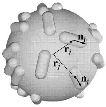
FIG. 3.: Spherical system. Each particle with position ${\bf r}_{i}$ and orientation ${\bf n}_{i}$ is forced to lie tangentially on the surface of a sphere.

FIG. 4.: Model of aligned rods. Each particle (discorectangles) has an orientation according to a prescribed director field (lines). The position of the arising $1/2$-defect is indicated by a filled circle, the orientation by an arrow.

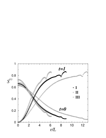
FIG. 5.: Nematic order parameters $S^{(t)}$ as a function of the radial distance $r$ from the droplet center, scaled by the rod length $L$. Star order $S^{(1)}$ and bulk order $S^{(0)}$ is shown. System (I) is reference, (II) has halved and (III) has doubled particle number. See Tab.I for a compilation of system parameters. Error bars are only given for (I).

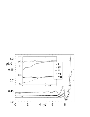
FIG. 6.: Radially resolved density profiles $\rho(r)$ as a function of the distance from the droplet center $r$ scaled by the particle length $L$. System (I) is reference, compared to lower (IV) and higher (V) packing fraction, and lower (VI) and higher (VII) anisotropies. The inset shows the behavior near the origin where a density decrease for (V) and (VII) appears for $r<2L$.

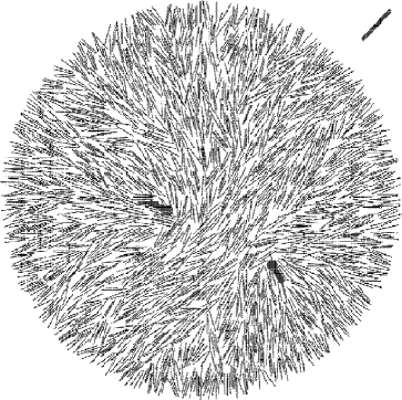
FIG. 7.: Snapshot of a typical particle configuration for the planar system (I). The particles are rendered dark. The two black symbols inside the droplet indicate positions and orientations of defects. The black bar outside the droplet indicates the global nematic director ${\bf q}^{(0)}$.

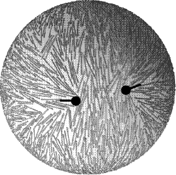
FIG. 8.: Snapshot of a typical particle configuration for the spherical system. The particles are rendered dark. There is one 1/2-defect on the left side and one on the right side. They point away from each other.

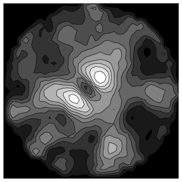
FIG. 9.: Order parameter $\lambda^{(\frac{1}{2})}$ as a function of spatial coordinates $r_{x},r_{y}$. Bright areas correspond to large values, dark areas correspond to small values of $\lambda^{(\frac{1}{2})}$. The two bright spots near the center are identified as topological defects, the gray islands as bulk defects.

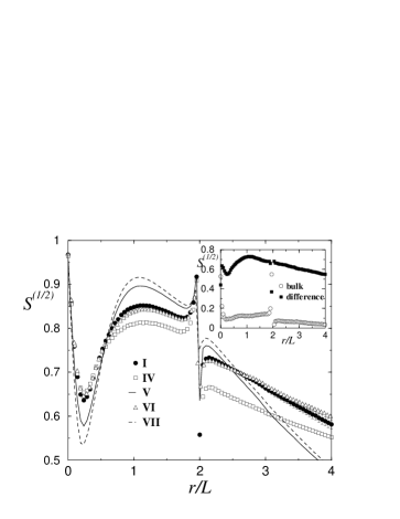
FIG. 10.: Order parameter profiles $S^{(\frac{1}{2})}$ around the defect center as a function of the scaled distance $r/L$ from the defect center. The reference system (I) is to be compared with lower (IV) and higher (V) packing fraction, and lower (VI) and higher (VII) anisotropies. The inset shows $S^{(\frac{1}{2})}$ for bulk defects and for the difference between (I) and the bulk.

FIG. 11.: Density profile as a function of the distance from the defect center. System (I) is reference, (II) has fewer particles, (III) has more. The spherical and aligned models are shown.

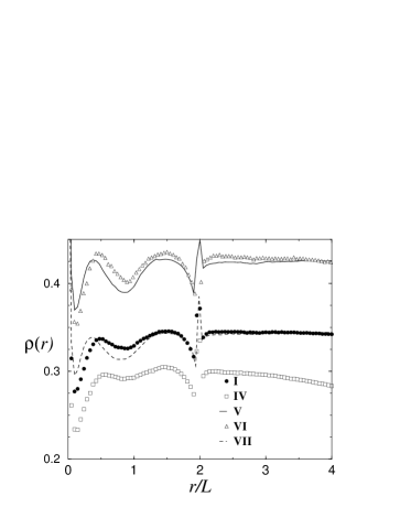
FIG. 12.: Same as Fig.11, but for lower (IV) and higher (V) packing fraction and shorter (VI) and longer particles (VII), compared to system (I).

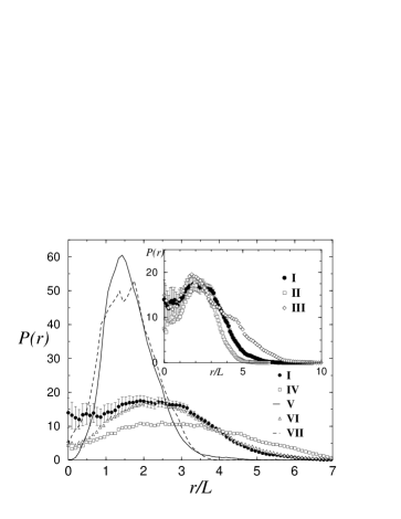
FIG. 13.: Probability distribution $P(r)$ for the distance of a defect from the center of the droplet $r/L$, for lower (IV) and higher (V) packing fraction and shorter (VI) and longer particles (VII), compared to system (I). The inset shows the the finite size behavior for halved (II) and doubled (III) particle number.

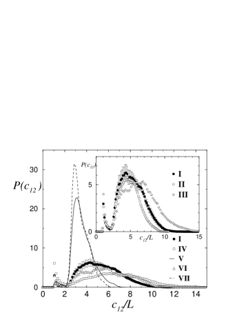
FIG. 14.: Probability distribution $P(c_{12})$ for the separation distance between both defect positions scaled by the particle length for lower (IV) and higher (V) packing fraction and shorter (VI) and longer spherocylinders (VII), as compared to system (I). The inset shows the finite size behavior for halved (II) and doubled (III) particle number compared to (I).

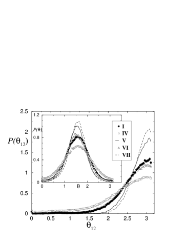
FIG. 15.: Probability distribution $P(\theta_{12})$ for the difference angle between both defect orientations. The reference system (I) is to be compared with lower (IV) and higher (V) packing fraction, and lower (VI) and higher (VII) anisotropies. The inset shows the distribution $P(\theta)$ of the difference angle between the direction of one of the defects and the global nematic director for the same parameters.

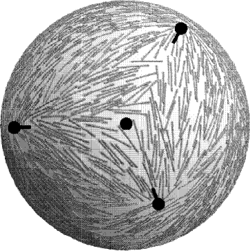
FIG. 16.: Triangular configuration of three positive defects around a spontaneously formed negatively charged defect (central dot).

REFERENCES

- [1] G. J. Vroege and H. N. W. Lekkerkerker, Reports on Progress in Physics 55, 1241 (1992).
- [2] L. Herbst, J. Kalus, and U. Schmelzer, J. Phys. Chem. 97, 7774 (1993).
- [3] G. Fröba and J. Kalus, J. Phys. Chem. 99, 14450 (1995).
- [4] S. Chandrasekhar, Liquid Crystals, Cambridge University Press, London, 1977.
- [5] C. Chiccoli, P. Pasini, and F. Semeria, Phys. Letters A 150, 311 (1990).
- [6] E. Berggren, C. Zannoni, C. Chiccoli, P. Pasini, and F. Semeria, Phys. Rev. E 50, 2929 (1994).
- [7] E. Berggren, C. Zannoni, C. Chiccoli, P. Pasini, and F. Semeria, Phys. Rev. E 49, 614 (1994).
- [8] M. P. Allen, M. A. Warren, M. R. Wilson, A. Sauron, and W. Smith, J. Chem. Phys. 105, 2850 (1996).
- [9] J. Stelzer, L. Longa, and H.-R. Trebin, J. Chem. Phys. 103, 3098 (1995).
- [10] M. P. Allen, G. T. Evans, D. Frenkel, and B. M. Mulder, Adv. Chem. Phys. LXXXVI, ed. by I. Prigogine and S. A. Rice , p. 1 (1993).
- [11] L. Onsager, Ann. N. Y. Acad. Sci. 51, 627 (1949).
- [12] P. Bolhuis and D. Frenkel, J. Chem. Phys. 106, 666 (1997).
- [13] H. Graf and H. Löwen, J. Phys. Condens. Matter 11, 1435 (1999).
- [14] H. Graf, H. Löwen, and M. Schmidt, Prog. Col. Polym. Science 107, 177 (1997).
- [15] Z. Bradac, S. Kralj, and S. Zumer, Phys. Rev. E 58, 7447 (1998).
- [16] A. Borstnik and S. Zumer, Phys. Rev. E 56, 3021 (1997).
- [17] T. Gruhn and M. Schoen, Phys. Rev. E 1997, 2861 (1997).
- [18] R. Sear, Phys. Rev. E 57, 1983 (1998).
- [19] P. C. Schuddeboom and B. Jérôme, Phys. Rev. E 56, 4294 (1997).
- [20] R. van Roij, M. Dijkstra, and R. Evans, Europhys. Lett 49, 350 (2000).
- [21] B. Groh and S. Dietrich, Phys. Rev. E 59, 4216 (1999).
- [22] S. Ramaswamy, R. Nityananda, V. A. Raghunathan, and J. Prost, Mol. Cryst. Liq. Cryst. 288, 175 (1996).
- [23] F. Alouges and B. D. Coleman, J. Phys. A 32, 1177 (1999).
- [24] P. Poulin, N. Francés, and O. Mondain-Monval, Phys. Rev. E 59, 4384 (1999).
- [25] A. N. Semenov, Europhys. Lett. 46, 631 (1999).
- [26] D. Pettey, T. C. Lubensky, and D. Link, Liq. Cryst. 25, 579 (1998).
- [27] N. D. Mermin, Rev. Mod. Phys. 51, 591 (1979).
- [28] M. Hindmarsh, Phys. Rev. Lett. 75, 2502 (1995).
- [29] W. Wang, T. Shiwaku, and T. Hashimoto, J. Chem. Phys. 108, 1618 (1998).
- [30] N. Schopohl and T. J. Sluckin, Phys. Rev. Lett. 59, 2582 (1987).
- [31] N. Schopohl and T. J. Sluckin, J. Phys. France 49, 1097 (1988).
- [32] C. Chiccoli, P. Pasini, F. Semeria, T. J. Sluckin, and C. Zannoni, J. Phys. II France 5, 427 (1995).
- [33] P. Biscari, G. G. Peroli, and T. J. Sluckin, Mol. Cryst. Liq. Cryst. 292, 91 (1997).
- [34] A. Sonnet, A. Kilian, and S. Hess, Phys. Rev. E 52, 718 (1995).
- [35] W. Huang and G. F. Tuthill, Phys. Rev. E 49, 570 (1994).
- [36] M. Ambroẑic, P. Formoso, A. Golemme, and S. Zumer, Phys. Rev. E 56, 1825 (1997).
- [37] F. Xu, H.-S. Kitzerow, and P. P. Crooker, Phys. Rev. E 49, 3061 (1994).
- [38] J. Bajc, J. Bezić, and S. Zumer, Phys. Rev. E 51, 2176 (1995).
- [39] M. Zapotocky and P. Goldbart, cond-mat/9812235, to be published, 1999.
- [40] J. A. Reyes, Phys. Rev. E 57, 6700 (1998).
- [41] A. P. J. Emerson and C. Zannoni, J. Chem. Soc. Farad. Trans. 91, 3441 (1995).
- [42] P. Poulin, H. Stark, T. C. Lubensky, and D. A. Weitz, Science 275, 1770 (1997).
- [43] H. Stark, (1999), to be published.
- [44] T. C. Lubensky, D. Pettey, N. Currier, and H. Stark, Phys. Rev. E 57, 610 (1998).
- [45] M. Zapotocky, L. Ramos, P. Poulin, T. C. Lubensky, and D. A. Weitz, Science 283, 209 (1999).
- [46] J. Ignés-Mullol, J. Baudry, L. Lejcek, and P. Oswald, Phys. Rev. E 59, 568 (1999).
- [47] D. Andrienko and M. P. Allen, Phys. Rev. E 61, 504 (2000).
- [48] S. D. Hudson and R. G. Larson, Phys. Rev. Lett. 70, 2916 (1993).
- [49] H. Löwen, Phys. Rev. E 50, 1232 (1994).
- [50] D. Frenkel and R. Eppenga, Phys. Rev. A 31, 1776 (1985).
- [51] J. Viellard-Baron, J. Chem. Phys. 56, 4729 (1972).
- [52] J. A. Cuesta and D. Frenkel, Phys. Rev. A 42, 2126 (1990).
- [53] P. van der Schoot, J. Chem. Phys. 106, 2355 (1997).
- [54] H. Schlacken, H.-J. Mögel, and P. Schiller, Mol. Phys. 93, 777 (1998).
- [55] M. J. Maeso and J. R. Solana, J. Chem. Phys. 102, 8562 (1995).
- [56] A. Chamoux and A. Perrera, Phys. Rev. E 58, 1933 (1998).
- [57] M. P. Allen, Mol. Phys. 96, 1391 (1999).
- [58] Z. T. Németh and H. Löwen, J. Phys. Condens. Matter 10, 6189 (1998).
- [59] Z. T. Németh and H. Löwen, Phys. Rev. E 59, 6824 (1999).
- [60] A. González, J. A. White, F. L. Román, S. Velasco, and R. Evans, Phys. Rev. Lett. 79, 2466 (1997).
- [61] A. González, J. A. White, F. L. Román, and R. Evans, J. Chem. Phys. 109, 3637 (1998).
- [62] A. M. Bohle, R. Holyst, and T. A. Vilgis, Phys. Rev. Lett. 76, 1396 (1996).
- [63] M. P. Allen and D. J. Tildesley, Computer Simulation of Liquids, Oxford University Press, Oxford, 1987.
- [64] K. Zahn, R. Lenke, and G. Maret, Journal de Physique II 4, 555 (1994).
- [65] K. Zahn and G. Maret, Curr. Opinion in Coll. Interf. Sci. 4, 60 (1999).