Contrasts between Equilibrium and Non-equilibrium Steady states:
Computer Aided Discoveries in Simple Lattice Gases

Abstract

A century ago, the foundations of equilibrium statistical mechanics were laid. For a system in equilibrium with a thermal bath, much is understood through the Boltzmann factor, $e^{-{\cal H[C]}/kT}$, for the probability of finding the system in any microscopic configuration ${\cal C}$. In contrast, apart from some special cases, little is known about the corresponding probabilities, if the same system is in contact with more than one reservoir of energy, so that, even in stationary states, there is a constant energy flux through our system. These non-equilibrium steady states display many surprising properties. In particular, even the simplest generalization of the Ising model offers a wealth of unexpected phenomena. Mostly discovered through Monte Carlo simulations, some of the novel properties are understood while many remain unexplained. A brief review and some recent results will be presented, highlighting the sharp contrasts between the equilibrium Ising system and this non-equilibrium counterpart.

PACS: 64.60Cn, 66.30Hs, 05.70Fh, 82.20Mj
Key words: non-equilibrium statistical mechanics, lattice gas, driven diffusive systems, Monte Carlo, phase transitions

I Introduction

As we celebrate the centennial of the American Physical Society, we honor the founding of equilibrium statistical mechanics, which also took place about a century ago. That breakthrough enables us to understand thermodynamics in terms of microscopics. Further, predictions based on the Boltzmann-Gibbs framework have been applied with so much success that we now take for granted many of the inventions of the industrial revolution, e.g., automobiles, 747’s, power stations, etc. Yet, it may be argued that no systems are truly “in equilibrium”, since infinite times and infinite thermal reservoirs or perfect insulations would be necessary. Indeed, essentially all natural phenomena bear the marks of non-equilibrium processes. Unlike the aforementioned class of “artificial” systems, most natural systems are not “set up” with special conditions, under which equilibrium statistical mechanics provides excellent approximations. Unfortunately, the theory of non-equilibrium statistical mechanics is far less developed than its equilibrium counterpart. As a result, the most ubiquitous phenomena are the most poorly understood. In fact, relying on the intuition from equilibrium physics, we are often surprised, even by the behavior of systems in non-equilibrium steady states. These form a small subset of non-equlibrium phenomena where the states are time-independent, mimicking systems in equilibrium. In this article, the main differences between systems in equilibrium and non-equilibrium steady states will be highlighted. For example, stationary distributions of the former are well known. In contrast, we have no simple Boltzmann-like factor, $e^{-{\cal H}/k_{B}T}$, for non-equilibrium steady states. Fortunately, with the aid of modern computers, it is possible to explore the behavior of simple model systems in stationary states far from equilibrium. An excellent example is the driven Ising lattice gas. Despite its simplicity, simulations continue to reveal a seemingly unending list of counter-intuitive phenomena. Yet, because of its simplicity, some of these surprises are now reasonably well understood.

From textbooks, we learn that the first step in equilibrium statistical mechanics is to apply the fundamental hypothesis to a physical system in complete isolation: every configuration, ${\cal C}$ (or microstate), available to the system may be found with equal probability: $P_{iso}[{\cal C}]\propto 1$. By energy conservation, ${\cal H[C]}$ (the energy associated with ${\cal C}$, which may include external static potentials) cannot change, i.e., $\Delta{\cal H\equiv}0$ . Extending our scope to a system which can exchange energy with a much larger (theoretically infinte) reservoir and applying the fundamental hypothesis to the combination, we arrive at the canonical ensemble: when equilibriated, the probability for finding a system in ${\cal C}$, $P_{eq}[{\cal C}]$, is proportional to $\exp(-{\cal H[C]}/k_{B}T)$, where $T$ is the temperature associated with the thermal reservoir. In this stationary state, on the average, the energy of our system is a constant, which may be denoted by $\left\langle\Delta{\cal H}\right\rangle_{T}=0$. Fluctuations around this constant can be traced to losses or gains to the reservoir, while the average energy flux between them is zero.

Here, we are interested in a system exchanging energies with two or more reservoirs, which are not coupled otherwise. If, say, the reservoirs are set at different temperatures initially, then we may expect the following scenario. Assuming the reservoirs are much larger than our system, then there should be a time when our system would be in a stationary state, while the reservoirs are still close to their initial states. In this sense, the combined system is far from equilibrium, with energy flowing from the hotter reservoir to the colder one. However, if we focus on our system alone, we find that its energy is constant on the average. Keeping in mind the presence of two reservoirs (for which we use the subscripts $T$ and $E$), we denote this situation by $\left\langle\Delta{\cal H}\right\rangle_{T}+\left\langle\Delta{\cal H}\right\rangle_{E}=0$. This state is also far from the equilibrium state, since there is a non-zero flux flowing through it. On the average, it gains a non-trivial amount of energy from one reservoir and loses energy to the other. In other words, neither term in the above equation vanishes: $\left\langle\Delta{\cal H}\right\rangle_{T}=-\left\langle\Delta{\cal H}\right\rangle_{E}{\cal\neq}0$. We will refer to such systems as being in non-equilibrium steady states. Examples abound in nature, from our planet as a whole to simple daily activities like cooking. The fundamental question for these states is: what is the stationary distribution $P^{*}[{\cal C}]$?

Because our problem is inherently a time dependent one, we believe that the most appropriate approach is to start with the $t$-dependent distribution: $P[{\cal C};t],$ the time evolution of which is governed by the master equation:

$$\frac{\partial}{\partial t}P[{\cal C};t]=\sum_{{\cal C}^{\prime}}\left\{R\left({\cal C}^{\prime}\rightarrow{\cal C}\right)P[{\cal C}^{\prime};t]-R\left({\cal C}\rightarrow{\cal C}^{\prime}\right)P[{\cal C};t]\right\}\equiv{\mathbb{L}}P.$$ (1)

Here $R\left({\cal C}\rightarrow{\cal C}^{\prime}\right)$ stands for the rate with which a configuration ${\cal C}$ changes to ${\cal C}^{\prime}$ and, in principle, can be found once we specify how our system is coupled to the various reservoirs. Then, the stationary $P^{*}$ will be “just” the (right) eigenvector of ${\mathbb{L}}$ with zero eigenvalue: $0={\mathbb{L}}P^{*}.$

For physical systems, the task of finding the $R$’s is clearly too complex. On the other hand, the success of equilibrium statistical mechanics suggests those $P^{*}$’s are independent of the details of the rates. Apart from mixing (all the configurations being connected by the $R$’s), the condition on the rates so that our system arrives at thermal equilibrium (being coupled to a single reservoir at temperature $T$) is known as detailed balance:

$$\frac{R\left({\cal C}^{\prime}\rightarrow{\cal C}\right)}{R\left({\cal C}\rightarrow{\cal C}^{\prime}\right)}=\exp\left\{\frac{{\cal H[C}^{\prime}{\cal]}-{\cal H[C]}}{k_{B}T}\right\}$$ (2)

Numerous successful Monte Carlo simulations of systems in equilibrium are based on choosing the Metropolis rate [1]: $R\left({\cal C}\rightarrow{\cal C}^{\prime}\right)=\min[1,e^{-({\cal H[C}^{\prime}{\cal]}-{\cal H[C]})/k_{B}T}].$ It is clear that, with rates satisfying eqn.(2), the Boltzmann $P_{eq}$ is a stationary distribution. Moreover, the equation $0={\mathbb{L}}P_{eq}$ is satisfied by

$\displaystyle R\left({\cal C}^{\prime}\rightarrow{\cal C}\right)P_{eq}\left({\cal C}^{\prime}\right)=R\left({\cal C}\rightarrow{\cal C}^{\prime}\right)P_{eq}\left({\cal C}\right)$

for every pair $\left({\cal C}^{\prime},{\cal C}\right)!$

An important distinction for a system evolving toward non-equilibrium steady states is that eqn.(2) no longer holds. The effects of two reservoirs cannot be embodied in eqn.(2). The stationary distribution $P^{*}$ is not known without solving $0={\mathbb{L}}P^{*}$ first while each term on the right hand side of eqn.(1) is not necessarily zero. A good analogue with electromagnetism is to regard eqn.(1) as a continuity equation. Then each ${\cal C}$ is analogous to a node in a circuit while the terms on the right are net currents between pairs of nodes. While equilibrium corresponds to electrostatics (with time-independent charge distribution and zero currents), non-equilibrium steady states correspond to magnetostatics, for which currents are steady but non-vanishing. Given this sharp contrast between equilibrium and non-equilibrium steady states, it is not surprising that the latter problem is considerably more difficult, since $P^{*}$ itself is unknown a priori. On the other hand, the variety and richness is also much greater. In general, $P^{*}$ will depend on the details of the rates, although we expect the “universality classes” of $R$’s leading to the same $P^{*}$ to be just as large as in the equilibrium case. In this short article, we will focus only on a particularly simple model – the driven Ising lattice gas [2]. Though the model appears simple, there is no analytic solution, so that its properties are generally explored through computer simulations. Now, most non-equilibrium systems are not translationally invariant. Typically, temperature gradients or velocity shears are present, so that the usual thermodynamic limits cannot be taken. As a result, the co-operative behavior in such systems is much more difficult to analyse than that in systems with translational invariance. An advantage of our simple model is that not only is it translationally invariant, it displays a host of surprising phenomena when driven to non-equilibrium steady states. In the next section, we will present a brief summary of the specifications of this model and some of the remarkable discoveries from Monte Carlo simulation studies. In many situations, the well honed arguments of equilibrium statistical mechanics, based on the competition between energy and entropy, fail dramatically. More details may be found in, e.g., [3]. Section 3 is devoted to some recent developments while some concluding remarks are included in the last.

II A Brief Review of the Driven Lattice Gas

Motivated by the physics of fast ionic conductors [4], Katz, Lebowitz and Spohn introduced a simple model in 1983 [2], which has served as a primary testing ground for exploring unusual properties of non-equilibrium steady states. It consists of an Ising lattice gas [5, 6] with attractive nearest-neighbor interactions, driven far from equilibrium by an external “electric” field, $E$. In the spin language, it is a ferromagnetic Ising model with biased spin-exchange [7] dynamics. Major reasons for choosing this model are:
$\cdot\$having a translationally invariant dynamics, the steady state is expected to be also invariant;
$\cdot\$the two reservoirs are coupled through an anisotropic dynamics;
$\cdot\$many of its equilibrium properties are well-known, especially in two dimensions ($d=2$) [8, 9];
$\cdot\$it is a system with non-trivial phases in $d>1$, whether driven or not;
$\cdot\$the equilibrium system can be reached continuously by taking the $E\rightarrow 0$ limit; and
$\cdot\$a different equilibrium system can be reached by choosing appropriate boundary conditions.
For completeness, we give a brief description of the $d=2$ model here. On a square lattice with fully periodic boundary conditions, each of the $L_{x}\times L_{y}$ sites may be occupied by a particle or left vacant, so that a configuration ${\cal C}$ of our system is completely specified by the occupation numbers $\{n_{i}\}$, where $i$ is a site label and $n$ is either 1 or 0. Translating the spin language of Ising[5] is simple: $s\equiv 2n-1=\pm 1$. An attractive interaction between pairs of particles in nearest-neighbor sites is modeled by the usual Hamiltonian: ${\cal H[C]}=-4J\sum_{<i,j>}n_{i}n_{j}$, with $J>0$. The factor of 4 means that ${\cal H}$ assumes the form $-J\sum ss$ in the spin language, so that, in the thermodynamic limit, the system undergoes a second order phase transition at the Onsager [8] critical temperature $T_{O}=(2.2692..)J/k_{B}$. For the lattice gas, this point can be reached only for half-filled systems, i.e., $\sum_{i}n_{i}=$ $L_{x}L_{y}/2$. In Monte Carlo simulations for a lattice coupled to a thermal bath at temperature $T$, particles are allowed to hop to vacant nearest neighbor sites with probability $\min[1,e^{-\Delta{\cal H}/k_{B}T}]$ [1], where $\Delta{\cal H}$ is the change in ${\cal H}$ after the particle-hole exchange. Note that these rules conserve the total particle number $\sum_{i}n_{i}$, so that half-filled lattices must be used, if critical behavior is to be studied. Starting from some initial state, this dynamics should bring the system into the equilibrium state with stationary distribution $P_{ce}[{\cal C}]\propto e^{-{\cal H[C]}/k_{B}T}$.

The deceptively simple modification introduced by Katz, et. al. [2] is an external “electric” field. Pretending the particles are “charged”, the effect of the drive is to modify the hopping rates to biased ones. Specifically, the jump probabilities are now $\min[1,e^{-(\Delta{\cal H}-\epsilon E)/k_{B}T}]$, where $\epsilon=(-1,0,1)$, for a particle attempting to hop (against, orthogonal to, along) the drive and $E$ is the strength of the field. Note that, locally, the effect of the external field is identical to that due to gravity. Indeed, had we imposed “brick wall” boundary conditions (particles reflected at the boundary, comparable to a floor or a ceiling), this system would eventually settle into an equilibrium state, like gas molecules in a room on earth. Of course, the reason behind this outcome is that gravitation is a static potential and can be incorporated into ${\cal H[C]}$. The “price” paid is the loss of translational invariance due to the presence of boundaries, leading to inhomogeneous particle densities.

Returning to our model, in which periodic boundary conditions are imposed, we see that translational invariance is completely restored so that, in the final steady state, the particle density is homogeneous, for all $T$ above some finite critical $T_{c}$. At the same time, a particle current will be present. For gravity, such a situation exists only in art [10]. In physics, this situation can be realised only with an electric field. Thanks to Faraday, a constant electric field circulating around the surface of a cylinder can be set up by applying a linearly increasing, axial magnetic field. If the particles are charged, they will experience the same force everywhere on the cylinder. As they also lose energy to the thermal bath, a steady state with finite current can be established. With this possibility in mind, we will use the term “electric” field to describe the external drive and imagine our particles to be “charged”. We should caution the reader that, unlike real charges, our particles are not endowed with Coulomb interactions between them, just like the typical neglect of gravitational attraction between gas molecules. Finally, note that a well defined, single-valued, potential which gives rise to such an electric field is necessarily time dependent.

Given the microscopic model, we can ask: What are its collective properties when it settles down in a non-equilibrium steady state? In particular, what is $P^{*}[{\cal C}]$? Since there is no global Hamiltonian, we cannot exploit Boltzmann’s result. Instead, we must resort to the master equation (1) and attempt to find the solution to $0={\mathbb{L}}P^{*}.$ Though ${\mathbb{L}}$ is a sparse matrix, finding $P^{*}$ is a non-trivial task. Only for very small systems can $P^{*}$ be obtained [11]. Of course, it is difficult to discern collective behavior such as phase transitions in “microscopic” systems like these. Nevertheless, we can already see that the $P^{*}$’s here (fig. 1a) are quite distinct from $P_{eq}$ (fig. 1b). Also, at this level, we can derive an interesting consequence: the violation of the standard fluctuation dissipation theorem. Computing $\left\langle{\cal H}\right\rangle$ and $\left\langle{\cal H}^{2}\right\rangle$, it is easy to verify that, in the driven case, $\left\langle{\cal H}^{2}\right\rangle-\left\langle{\cal H}\right\rangle^{2}\neq-\partial_{\beta}\left\langle{\cal H}\right\rangle.$

Turning to collective phenomena on the macroscopic scale, we face serious difficulties in finding $P^{*}$ analytically, let alone solving for thermodynamic quantities a la Onsager. Without modern computers, it would be impossible to make much progress. Using simulation techniques, we may answer questions like: what happens to the second order phase transition found by Onsager? In particular, how does the critical temperature depend on the drive, i.e., what is $T_{c}(E)$? Several simple possibilities come to mind:
a) $T_{c}(E)$ jumps to infinity for any $E$ , i.e., the drive, however small, orders the system.
b) $T_{c}(E)$ rises with $E$ indefinitely.
c) $T_{c}(E)$ rises with $E$, saturating at some finite temperature $T_{c}(\infty)$.
d) $T_{c}(E)$ is independent of $E$ , i.e., $T_{c}(E)=T_{O}$.
e) $T_{c}(E)$ decreases with $E$, either dropping to zero at finite $E$, or saturating at a finite $T_{c}(\infty)$.
f) $T_{c}(E)$ jumps to zero for any $E$ , i.e., the drive, however small, disorders the system.
While possibilities (a), (b), and (f) appear incredulous, intuitive arguments might be made for (d) and (e). The naive argument for (d) is that, in an inertial frame where the global current vanishes, the system should look just like an equilibrium Ising model. On the other hand, to arrive at (e), we think of the drive as gravity, feeding energy into the system, so that its effects should be the same as a reservoir with a temperature higher than the surrounding bath. Therefore, to order the system, the bath temperature would have to lowered, i.e., $T_{c}(E)<T_{O}$. In reality, simulations [2] offered the first surprise: $T_{c}(E)$ increasing with $E$ and saturating at $T_{c}(\infty)\simeq 1.4T_{O}$ [12]! A number of arguments now exists for this behavior, but all are “post-dictions”. Indeed, none of these are convincing, while approximate schemes for analytic computations of $T_{c}(E)$ offer only hints to the puzzle of $T_{c}(E)>T_{c}(0)$ [13, 14].

As the system is probed deeper, more surprises appear. Due to space limitations, we only list some of them here, refering the interested reader to [3, 15] for further details.

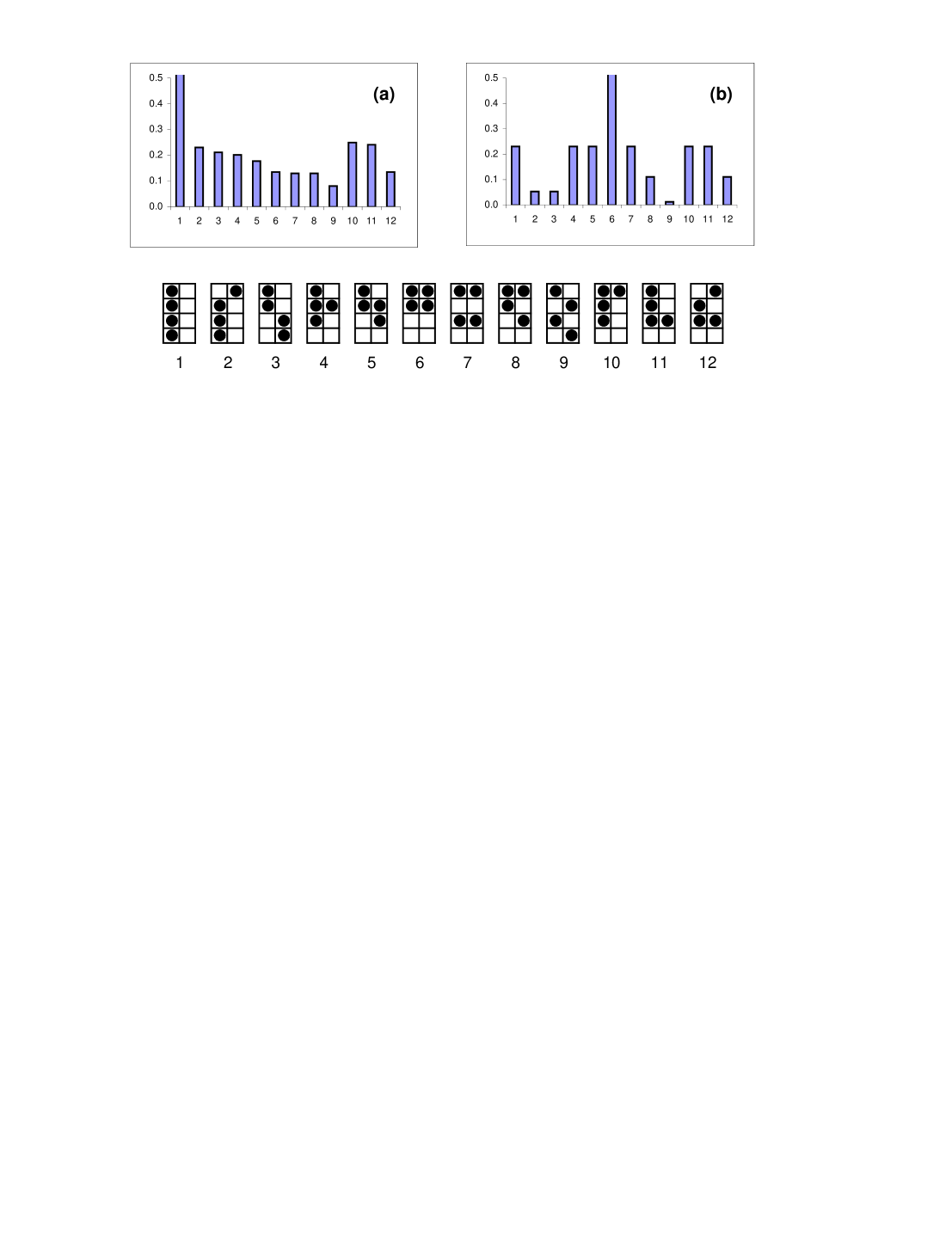
FIG. 1.: Stationary distributions for a 4$\times$2 Ising lattice gas, driven with infinite $E$ (a) and in equilibrium (b). The normalization is set via: largest $P^{*}\equiv 1$. Corresponding configurations (only one out of the equivalence class) are shown, with the drive downwards.

A Disordered phase ($T>T_{c}$)

In the equilibrium system, there is little of interest far above criticality. Correlations are short ranged so that most properties can be understood through Landau-Ginzburg mean field theory. When driven, however, this system displays
$\cdot\$long range two-point correlations, decaying as $1/r^{d}$ [16]
$\cdot\$singular structure factors, with a discontinuity at the origin [2, 17]
$\cdot\$non-trivial three point correlations, the Fourier transforms of which show infinite discontinuities at the origin [18];
$\cdot\$a fixed line, rather than the Gaussian fixed point, governing large-scale, long time behavior [19];
$\cdot\$shape-dependent thermodynamics[20]

B Critical Behavior ($T\sim T_{c}$)

In 1944, Onsager solved the $d=2$ Ising model and computed many of its critical properties. However, the deeper understanding of critical phenomena came only in the 70’s, with the advent of field theoretic renormalization group analysis[21]. Within this framework, we learnt that a large class of systems fall into the Ising universality class, controlled by the Wilson-Fisher fixed point[22]. When driven into non-equilibrium states,
$\cdot\$only ordering into strips parallel to $E$ occurs;
$\cdot\$only one of the two lowest structure factors diverges;
$\cdot\$strong anisotropy appears while longitudinal and transverse momenta scale differently;
$\cdot\$the critical dimension is 5 instead of 4;
$\cdot\$a new, non-Hamiltonian, fixed point and universality class is identified [23];
$\cdot\$a host of new exponents, though only one independent, emerges; and
$\cdot\$anisotropic finite size scaling is essential for data collapse [12].
We should note that, unlike properties far from $T_{c}$, the critical properties were predicted by theory [23] well before confirmations from computer simulation studies [12].

C Ordered phase ($T<T_{c}$)

Below the critical point, phase segregation and co-existence occurs, with interfaces separating the particle rich from the particle poor regions. Due to the periodic boundary conditions, each region is a single strip wrapped around the torus. Unlike in equilibrium, only strips parallel to the drive exist. Correlations within each region are also expected to be long ranged, though they have not been studied carefully so far. Some intriguing properties of the interfaces, dramatically different from equilibrium [24] ones, are:
$\cdot\$statistical widths remaining finite as $L\rightarrow\infty$ [25] rather than diverging as $\sqrt{L}$;
$\cdot\$the structure factor diverging as $q^{-0.67}$ [26] instead of the usual $q^{-2}$ of capillary waves[27]; $\cdot\$interface orientation affecting bulk energies [28]; and
$\cdot\$instabilities when forced to lie at a non-vanishing angle with respect to the drive[29].
In addition to interface anomalies, other remarkable features include
$\cdot\$coarsening during a quench showing several time regimes and asymmetries which cannot be accounted for by a modified Cahn-Hilliard theory [30];
$\cdot\$systems subjected to shifted periodic boundary conditions displaying new, multistrip phases [28]; and
$\cdot\$systems subjected to open periodic boundary conditions displaying icicle like fingers[31].

As we try to convey in this section, there are still many unresolved mysteries associated with this decepetively simple model. In the next section, we will present some recent, on-going investigations which attempt to probe deeper into the simple driven lattice gas.

III Some Recent Developments

A Steady State Energy Fluxes

In the introduction, we emphasized the importance of energy flow through our system in a non-equilibrium steady state. There has been no systematic study of this aspect, even though it may contain a key to the understanding of such systems. We begin by simply confirming our intuitive picture: that typical jumps parallel/trasverse to the field are associated with energy gain/loss. In the previous section, we showed the complete solution for a $4\times 2$ lattice. Using those $P^{*}$’s, we can compute these gains/losses and then compare them with Monte Carlo simulations [32]. The results are best displayed as histograms for all possible values of $\Delta{\cal H}$ after an attempted jump. There are two such histograms, associated with the two types of jumps. We also performed the same analysis for the equilibrium case. It is reassuring that simulations confirm, within statistical errors, all theoretical predictions. Encouraged by these results, we carried out simulations on a $30\times 30$ lattice [32]. Figure 2a shows that, for the equilibrium case, both histograms are entirely symmetric (within statistical errors), so that the gains/losses balance for either types of jumps. By contrast, figure 2b shows asymmetric histograms, confirming our expectation that the systems tends to gain energy when a particle jumps in the field direction, etc. Our hope is that a good approximation scheme, within the theoretical framework described above, can be found leading to quantitative predictions of these histograms.

B A Possible New Phase in Lattice Gases with Anisotropic Interactions

Since the drive introduces a non-trivial anisotropy into the Ising lattice gas, it is natural to ask how $E$ might compete with anisotropic couplings. The equilibrium model is part of Onsager’s solution, so that we may again compare driven cases with well-known results. Since the drive enhances longitudinal correlations, we had expected that “$T_{c}(E)$ will be higher (lower) if the drive is aligned with the stronger (weaker) bonds” [33]. Subsequent simulations showed the opposite[34]! Indeed, with saturation drive, $T_{c}(E)$ can drop below $T_{c}(0)$ for $\alpha\gtrsim 1.7$, where $\alpha^{2}$ is the ratio of the coupling along the field direction to the “transverse” coupling. Motivated to look into the behavior displayed at various temperatures, we find that the typical configurations are indeed disordered for $T\gg T_{c}(0)$ and ordered into a single strip for $T\ll T_{c}(E)$. However, there is a significant range of temperatures where the system appears to be “ordered” in the drive direction without being in a single strip. In other words, while the densities in each column (i.e., along the drive) are bi-modally distributed [35], the usual order parameter ($S(1,0)$, structure factor with lowest transverse wave number) is still quite small. In more picturesque language, we call this a “stringy” state. Actually, this type of configurations have been previously reported [36]. But they were believed to be long transients on the way from disordered initial states to ordered ones and thus, disregarded. By contrast, we observed that, starting from ordered states, the system evolves towards, and spends considerable periods of time in, the stringy states.

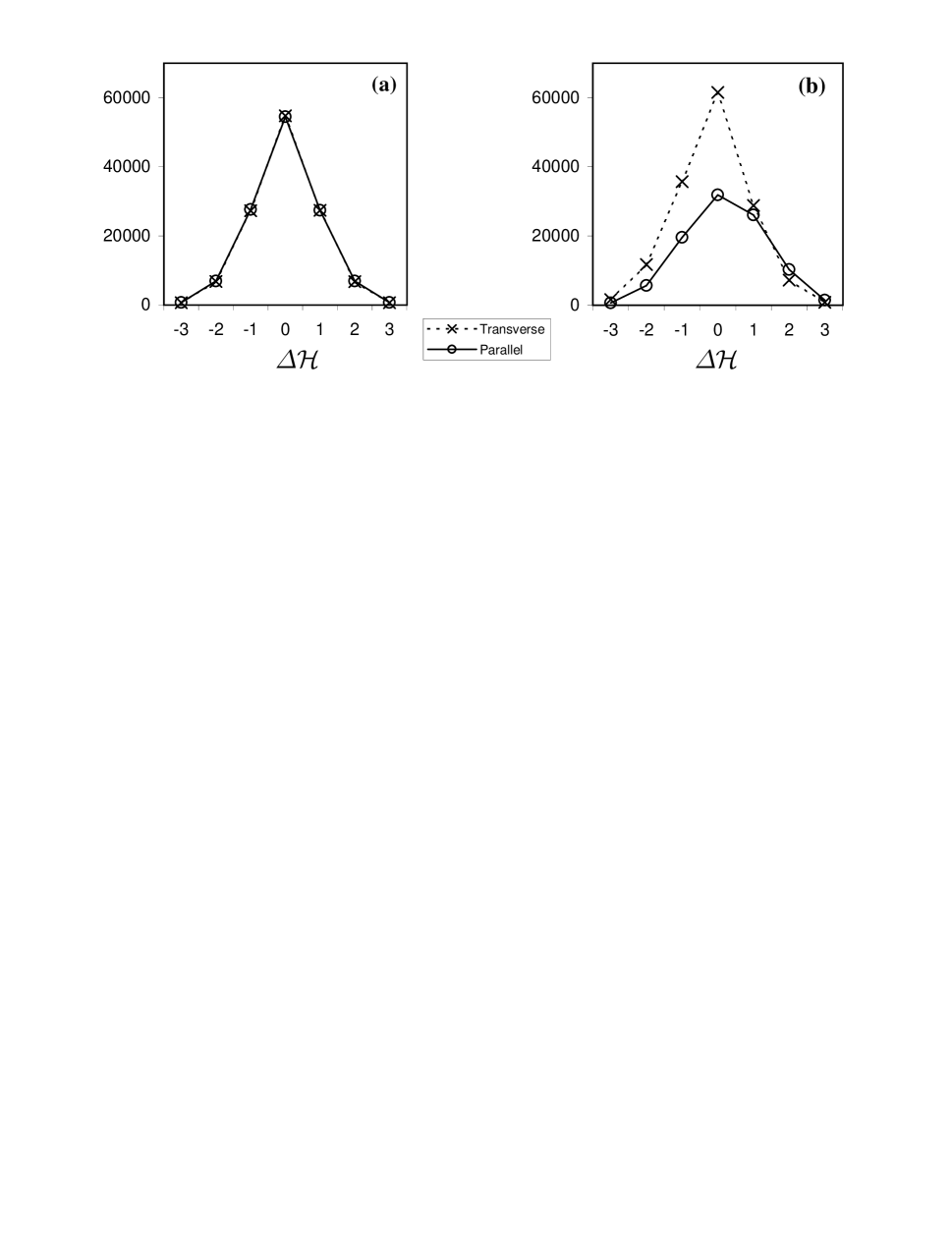
FIG. 2.: Histograms of $\Delta{\cal H}$ after an attempted jump in a $30\times 30$ lattice, at $T=2.5$ with $E=0$ (a) and $E=\infty$ (b).

In an effort to quantify these states, we define the ratio:

$${\cal R}\equiv L^{d}\frac{G(0,L/2)}{S(1,0)}$$ (3)

where $G(x,y)$ is the (untruncated!) two point correlation function, with $y$ being parallel to the drive, and $S(k,p)\equiv\sum_{x.y}G(x,y)e^{2\pi i\left(kx+py\right)/L}$ is the structure factor, used ordinarily as the order parameter. In particular, we are interested in the behavior of ${\cal R}$ as $L\rightarrow\infty$.

Far in the disordered phase, as a result of the $r^{-d}$ decay, we have $G(0,L/2)\rightarrow O(L^{-d})$ while $S(1,0)\rightarrow O(1)$. On the other hand, deep in the ordered phase $G\rightarrow O(1)$ while $S\rightarrow O(L^{d})$. Therefore, as long as the system is far from criticality, we have

$${\cal R}\rightarrow O(1).$$ (4)

Near criticality, if there are no stringy states, we may apply the results of renormalization group analysis [23] – $G(0,r)\rightarrow r^{-[d-2+\Delta]/(1+\Delta)}$ and $S(k,0)\rightarrow k^{-2}$ – to arrive at ${\cal R}\rightarrow L^{\left[d-3\right]\Delta/(1+\Delta)}$. Here, $\Delta$ is the exponent associated with anisotropic scaling of the momenta ($k_{\|}\sim k_{\bot}^{1+\Delta}$), and is found to be $(8-d)/3$ to all orders in the expansion around $(5-d\dot{)}>0.$ Thus, for our simulations in $d=2$, we see that ${\cal R}$ decreases with $L:$

$${\cal R}\rightarrow L^{-2/3}$$ (5)

By contrast, in a stringy state, ordering has set in for the longitudinal direction so that $G(0,L/2)\rightarrow O(1)$. Meanwhile, complete phase segregation into just two regions is yet to take place, so that $S(1,0)\rightarrow O(1)$. As a result, we expect

$${\cal R}\rightarrow L^{d}$$ (6)

which is an increasing function of $L.$ The differences between the three behaviors (4, 5, and 6) should be dramatic enough to discern in simulations.

To provide further contrast, we perform the above analysis for Ising models in equilibrium. Above criticality, $G\rightarrow e^{-r/\xi}r^{2-d}$ and $S\rightarrow O(1)$ so that ${\cal R}$ decreases exponentially as $L^{2}e^{-L/\xi}$. Near $T_{c},$ we have $G\rightarrow r^{2-d+\eta}$ and $S\rightarrow k^{-2+\eta}$ leading to ${\cal R}\rightarrow O(1)$. The behavior deep in the ordered phase is unchanged. So, in all cases, ${\cal R}$ should not increase with $L$.

Turning to simulations, we find that the stringy state seems to be most pronounced for large $\alpha.$ In particular, we focused on models with $\alpha=3$ and saturation drive and compiled data from systems sizes $L=10,20,30,40,60,$ and $90$, using two or three independent runs. Starting with both random and ordered initial conditions, the runs last up to 800,000 Monte Carlo steps. The plot of ${\cal R}$ vs. $L^{2}$ in figure 3 shows that, for two of the temperatures investigated, this ratio appears to be increasing with $L$. Meanwhile, for $T\notin\left[0.8,1.0\right]$, the behavior is consistent with ${\cal R}\rightarrow O(1)$. These preliminary results lead us to conjecture the existence of a “stringy phase”, especially in the thermodynamic limit of square ($L\times L$) lattices. Of course, simulations with larger $L$’s will be needed to determine if the increasing behavior persists. Other systematic methods can also be brought to bear, such as distribution functions of both $G$ and $S$. We have initiated a study of the histograms of $S(k,p)$ for a range of low lying wave-vectors, using the time-series of each quantity. Preliminary data show remarkable structures which are being verified in longer runs. Attempts at a theoretical understanding, based on phenomenological approaches, of the nature of the “stringy phase” are in progress.

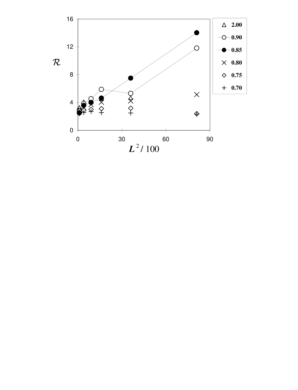
FIG. 3.: Correlation-Structure Factor ratio ${\cal R}$ for systems with $\alpha=3$ and saturation drive, plotted against $L^{2}.$ The legend refers to the temperatures of the various runs.

IV Concluding Remarks

In this brief article, we highlighted several major differences between a system in thermal equilibrium and one in non-equilibrium steady states. Apart from the obvious presence of non-trivial energy fluxes, the latter systems display many distinguishing and surprising features. Since their stationary distributions are neither a priori known nor susceptible to analytic probes (except for some simple limits or 1-D cases), all efforts to uncover the macroscopic, collective properties of these systems are based on Monte Carlo simulations.

Focusing on a particularly simple model – the Ising lattice gas, driven into non-equilibrium steady states by an external “electric” field[2], we gave a brief review of a variety of surprising and counter-intuitive behavior. In the last section, we offered two of the recent developments in this continuing saga: detailed investigations of the energy flux and preliminary studies indicating the possible existence of a new phase (especially for systems with large anisotropies in the attractive interactions). Beyond this simple model, many generalizations have been explored. Examples include repulsive interactions, random drives, quenched random impurities, multilayers, and multispecies, to name but a few [3]. Further from this class of “driven diffusive systems” is a wide range of other non-equilibrium steady states, e.g., surface growth, electrophoresis and sedimentation, granular and traffic flow, biological and geological systems, etc. All of these offer further surprises, some understood and most unexplained. At present, each non-equilibrium system is studied independently from the others. The hope is that a unifying concept and framework, like the fundamental hypothesis or the Boltzmann factor, will be discovered before the next centennial meeting of the APS.

V Acknowledgments

We are grateful to F.S. Lee for some unpublished work on the 4$\times$2 system. This research was supported in part by a grant from the National Science Foundation through the Division of Materials Research.

REFERENCES

- [1] N. Metropolis, A.W. Rosenbluth, M.M. Rosenbluth, A.H. Teller, and E. Teller, J. Chem. Phys. 21, 1087 (1953).
- [2] S. Katz, J. L. Lebowitz and H. Spohn, Phys. Rev. B 28, 1655 (1983); J. Stat. Phys. 34, 497 (1984).
- [3] For a more extensive review, see, e.g., B. Schmittmann and R. K. P. Zia, Phase Transitions and Critical Phenomena, Vol. 17, edited by C. Domb and J. L. Lebowitz (Academic, London, 1995).
- [4] See, e.g., S. Chandra, Superionic Solids. Principles and Applications (North Holland, Amsterdam 1981).
- [5] Ising, Z. Physik 31, 253 (1925). A more recent treatment is, e.g.,
- [6] C.N. Yang and T.D. Lee, Phys. Rev. 87, 404 (1952); and T.D. Lee and C.N. Yang, Phys. Rev. 87, 410 (1952).
- [7] K. Kawasaki, Ann. Phys. 61, 1 (1970).
- [8] L. Onsager, Phys. Rev. 65, 117 (1944) and Nuovo Cim. 6, (Suppl.) 261 (1949).
- [9] B. M. McCoy and T. T. Wu, The Two-dimensional Ising Model (Harvard Univ. Press, Cambridge, Mass., 1973).
- [10] In particular, see the lithograph Ascending and Descending, reproduced on the cover of [3].
- [11] M.Q. Zhang, Phys. Rev. A35. 2266 (1987).
- [12] K.-t. Leung, Phys. Rev. Lett. 66, 453 (1991) and Int. J. Mod. Phys. C3, 367 (1992); J. S. Wang, J. Stat. Phys., 82, 1409 (1996).
- [13] N.C. Pesheva, Y. Shnidman, and R.K.P. Zia, J. Stat. Phys. 70, 737 (1993).
- [14] B. Schmittmann and R. K. P. Zia, J. Stat. Phys. 91, 525 (1998).
- [15] B. Schmittmann and R. K. P. Zia, Phys. Rep. 301, 45 (1998).
- [16] M. Q. Zhang, J. -S. Wang, J. L. Lebowitz and J.L. Valles, J. Stat. Phys. 52, 1461 (1988); P. L. Garrido, J. L. Lebowitz, C. Maes and H. Spohn, Phys. Rev. A42, 1954 (1990).
- [17] R.K.P. Zia, K. Hwang, K-t. Leung, and B. Schmittmann, in Computer Simulation Studies in Condensed Matter Physics V, eds. D.P. Landau, K.K. Mon, and H.-B. Schüttler, (Springer, Berlin, 1993a).
- [18] K. Hwang, B. Schmittmann and R. K. P. Zia, Phys. Rev. Lett. 67, 326 (1991) and Phys. Rev. E48, 800 (1993).
- [19] H.K. Janssen and B. Schmittmann, Z. Phys. B63, 517 (1986); R.K.P. Zia and B. Schmittmann, Z. Phys. B97, 327 (1995).
- [20] F.J. Alexander and G.L. Eyink, Phys. Rev. E57, R6229 (1998) and G.L. Eyink,J.L. Lebowitz and H. Spohn, J. Stat. Phys. 83, 385 (1996).
- [21] See, e.g., K.G. Wilson, Rev. Mod. Phys. 47C, 773 (1975); D.J. Amit, Field Theory, the Renormalization Group and Critical Phenomena, 2nd revised edition, (World Scientific, Singapore, 1984); J. Zinn-Justin, Quantum Field Theory and Critical Phenomena, (Oxford University Press, Oxford, 1989).
- [22] K.G. Wilson and M.E. Fisher, Phys. Rev. Lett. 28, 240 (1972).
- [23] H.K. Janssen and B. Schmittmann, Z. Phys. B64, 503 (1986); K-t. Leung and J.L. Cardy, J. Stat. Phys. 44, 567 and 45, 1087 (Erratum) (1986).
- [24] See references in, e.g., R.K.P. Zia, in Statistical and Particle Physics: Common Problems and Techniques, eds. K.C. Bowler and A.J. McKane (SUSSP Publications, Edinburgh, 1984).
- [25] K.-t. Leung, K. K. Mon, J. L. Vallés and R. K. P. Zia, Phys. Rev. Lett. 61, 1744 (1988) and Phys. Rev. B39, 9312 (1989).
- [26] K.-t. Leung and R. K. P. Zia, J. Phys. A26, L737(1993).
- [27] F. P. Buff, R. A. Lovett and F. H. Stillinger, Phys. Rev. Lett., 15, 621 (1965).
- [28] J .L. Vallés, K.-t. Leung and R. K. P. Zia, J. Stat. Phys. 56, 43 (1989).
- [29] K-t. Leung, J. Stat. Phys. 50, 405 (1988) and 61, 341 (1990); C. Yeung, J.L. Mozos, A. Hernandez-Machado, D. Jasnow, J. Stat. Phys. 70. 1149 (1992).
- [30] C. Yeung, T. Rogers, A. Hernandez-Machado, D. Jasnow, J. Stat. Phys. 66. 1071 (1992); F.J. Alexander, C.A. Laberge, J.L. Lebowitz and R.K.P. Zia, J. Stat. Phys. 82, 1133 (1996); A. D. Rutenberg and C. Yeung, cond-mat/9903049, to be published.
- [31] D. H. Boal, B. Schmittmann and R. K. P. Zia, Phys. Rev. A43, 5214 (1991).
- [32] R. J. Astalos, to be published.
- [33] C.C. Hill, R.K.P. Zia and B. Schmittmann, Phys. Rev. Lett. 77, 514-517 (1996).
- [34] L.B. Shaw, B. Schmittmann, and R.K.P. Zia, cond-mat/9807057; to appear in J. Stat. Phys.
- [35] L.B. Shaw, Monte Carlo and Series Expansion Studies of the Anisotropic Driven Ising Lattice Gas Phase Diagram MS thesis, Virginia Polytechnic Institute and State University (May, 1999).
- [36] J.L. Vallés and J. Marro, J. Stat. Phys. 49, 89 (1987).