Facet ridge end points in crystal shapes

Abstract

Equilibrium crystal shapes (ECS) near facet ridge end points (FRE) are generically complex. We study the body-centered solid-on-solid model on a square lattice with an enhanced uniaxial interaction range to test the stability of the so-called stochastic FRE point where the model maps exactly onto one dimensional Kardar-Parisi-Zhang type growth and the local ECS is simple. The latter is unstable. The generic ECS contains first-order ridges extending into the rounded part of the ECS, where two rough orientations coexist and first-order faceted to rough boundaries terminating in Pokrovsky-Talapov type end points.

PACS number(s): 64.60 Fr, 68.35 Bs, 64.60 Ht, 68.35 Rh

Equilibrium crystal shapes (ECS) have been studied over the span of many years  [1]. Many features of their thermal evolution are theoretically well understood and have been observed experimentally. For example, surface roughening of facets are realizations the Kosterlitz-Thouless transition [1]. They have been observed in Helium crystals  [2], metal surfaces [3], ionic solids [4] and organic crystals [5]. Smooth boundaries between flat facets and rounded rough regions, like in Fig. 1(a), belong to the so-called Pokrovsky-Talapov (PT) universality class. They have been observed in, e.g., lead [6] and Helium crystals [7]. An aspect for which experimental data is still sparse is the ECS structure near facet ridge end point (FRE). For example, in NaCl crystals, facet ridges seem to vanish very quickly as temperature is increased [8]. Many other experiments reproduce growth shapes, where FRE points are not represented properly (rough surface orientations are suppressed because they grow faster than facets).

Lately the ECS structure near FRE points has gained theoretical attention, with the discovery of a link with Kardar-Parisi-Zhang (KPZ) type non-equilibrium growth [9]. Fig. 1(a) represents the simplest and until now canonical ECS structure near FRE points. The sharp ridge between two faceted orientations terminates and splits into two PT facet-to-round boundaries. This structure is realized in the so-called body-centered solid-on-solid (BCSOS) model with next-nearest neighbor interactions only [10], which is equivalent to the exactly solved six-vertex model. The FRE point where the PT lines join the facet ridge is very intriguing. At this point, the model can be mapped exactly onto a one dimensional BCSOS growth model that lies in the KPZ universality class [9]. To be more precise, the transfer matrix of the two dimensional equilibrium model maps onto the master equation of the one dimensional growth model. The spatial direction parallel to the facet ridge plays the role of time in the dynamic process.

This seems to settle the issue, but the FRE point in this exactly soluble model has too much symmetry (by being stochastic) to leave us confident that its scaling behavior is universal and that the ECS of Fig. 1(a) represents the generic shape. Recently, we performed a study of the ECS in a BCSOS model on a honeycomb lattice [11]. There we did not find the structure of Fig. 1(a), but instead shapes equivalent to Fig. 1 (b) and (c). In (b) the facet ridge extends into the rough region as a first-order rough-to-rough (FOR) line. It terminates at a critical end point. This possibility had been suggested before [10] but had not been observed in any model beyond mean field theory. Our result was somewhat unsatisfactory however since the FOR line remained extremely short. In another part of the phase diagram we found an ECS similar to Fig. 1(c). The boundaries between the faceted and the rounded rough regions are partially first-order. These segments became quite long and we could establish the scaling behaviour of the critical end points (PTE points) where the transition becomes PT like. PTE scaling is in agreement with a simple theory where the free energy is assumed analytic on the rough side and expandable in powers of the tilt angle [11, 12, 13]. PTE points have been observed in Si(113) [14], but with scaling exponents different from the above mean field type values. This can be attributed to long range attractive step-step interactions in the context of step bunching [13, 15].

In this letter, we present a study of the BCSOS model on the square lattice with enhanced interaction range. We address directly the stability of the stochastic FRE point. The FOR lines are well developed in this model. They appear also as stand-alone ridges inside the rounded parts of the crystal, as shown in Fig. 1(d), representing spontaneous symmetry breaking within the rough phase (coexistence between two rough surface orientations).

Consider a square lattice, oriented diagonally. The most general Hamiltonian with only next-nearest neighbor interactions, the one that is exactly soluble, can be written as

$$H_{0}=\sum_{x,y} [{1\over 4}L_{H}(h_{x+2,y}-h_{x,y}-E_{H}/L_{H})^{2}$$ (1)

$$+ {1\over 4}L_{V}(h_{x,y+2}-h_{x,y}-E_{V}/L_{V})^{2}]$$ (2)

with $x+2,y$ ($x,y+2$) and $x,y$ next nearest neighbors in the horizontal (vertical) direction and $h_{x,y}=0,\pm 1,\pm 2,\cdots$ the height variables. Nearest neighbor heights must differ by one. The fields $E_{H}$ and $E_{V}$ couple to the slopes, which we denote as $Q_{H}$ and $Q_{V}$ respectively. In this diagonal set up, the time like direction of the transfer matrix coincides with the facet ridges in Fig. 1. The ECS of this model takes the structure of Fig. 1(a) when $\exp(-L_{H})>\exp(-L_{V})+1$, in particular when the step-step interactions are attractive in the horizontal direction and repulsive in the vertical direction. The FRE point has the stochastic KPZ character mentioned above  [10, 9]. To study the stability of the stochastic FRE point we need to break the special symmetries of $H_{0}$. Increasing the interaction range will do this. We choose uniaxial interactions for numerical convenience. The simplest is to add interactions between next-to-next nearest neighbors lying in the same horizontal row

$$H=H_{0}+\sum_{x,y}[ M_{2}\,\delta(h_{x,y},h_{x+4,y}\pm 2)$$ (3)

$$+ M_{4}\,\delta(h_{x,y},h_{x+4,y}\pm 4)]$$ (4)

with $\delta(x)$ Kronecker delta’s. This involves two coupling constants, $M_{2}$ and $M_{4}$, because those further neighbors can differ in height by $0$, $\pm 2$, or $\pm 4$. The details of the numerical analysis are the same as in our previous paper [11] and outlined there in detail. The eigenvalues of the transfer matrix yield the exact free energy as function of tilt angle, $f(E_{V},Q_{H},N)$, at all temperatures in a semi-infinite strip geometry of width $N$. The ECS follows from this by a $N\to\infty$ finite size scaling analysis, combined with a Legendre transform. The latter is in essence the Wulff construction [16].

The phase diagram at $L_{H}=-0.69$ and $L_{V}=0.69$ for zero tilt fields, $E_{H}=E_{V}=0$, is shown in Fig. 2. This is a representative example. In the upper right corner, where $M_{2}$ and $M_{4}$ are both large and positive, the surface is flat. As $M_{4}$ is decreased, the surface undergoes a first-order transition to a faceted phase. The slope of the surface changes abruptly from $(0,0)$ to two coexisting $(Q_{H},Q_{V})=(\pm 1,0)$ facets. As $M_{2}$ is decreased, starting from the flat phase, the surface first roughens, via a KT transition and then enters a spontaneously tilted rough phase [17]. This is a rough-to-rough faceting transition with yet unknown anisotropic scaling properties. In the tilted phase, two rough phases coexist. The rounded part of the ECS contains a first-order ridge as shown in Fig. 1(d). The jump in orientation is caused by the competition between the $L$ and $M$ interactions, and changes continuously throughout this phase. It locks in smoothly to $Q_{H}=\pm 1$ at the PT boundary into the faceted phase.

The dashed line in Fig. 2 inside the faceted phase does not represent a phase transition. It marks the boundary between the two different shapes, Figs. 1 (b) and (c). In region (c), the edge between each facet and the rounded rough region is sharp near the FRE point. The scaling at the PTE point (where the edge becomes a conventional PT boundary) is consistent with our previous study, i.e., with an analytic free energy functional in terms of the surface tilt angle. The correlation length in the direction along the facet ridge scales compared to the perpendicular one as $\xi_{\parallel}\sim l_{\perp}^{z}$ with $z=3$  [11, 12, 13].

In region (b) the first-order facet ridge boundary between the $(\pm 1,0)$ facets extends into the rounded region as a FOR line, as shown in Fig. 1(b). Unlike our previous study on the honeycomb lattice [11], the FOR line becomes quite long and is unambiguously resolved. For example, at point $(L_{H},L_{V},M_{2},M_{4})=(-0.69,0.69,-0.02,0.02)$ the end point of the FOR line lies at $E_{V}=1.04\pm 0.01$, while the location of the FRE point is known exactly, $E_{V}=0.908$. At the phase boundary into the spontaneously tilted rough phase, the ECS changes from Fig. 1(c) to Fig. 1(d). In the latter the facet-to-round boundary never touches the FOR line.

The scaling behaviour at the FOR end point is an important issue. A naive guess is to assume the free energy is analytic in terms of the tilt angles. It should then take the asymptotic form $f(Q_{H},E_{V})=A(E_{V}-E_{V}^{*})Q_{H}^{2}+BQ_{H}^{4}$, such that at the FOR critical end point the free energy scales like $f\sim Q_{H}^{4}$. The free energy gap between the $Q_{H}=0$ and $Q_{H}=1/L$ sectors would behave as $L[f(1/L)-f(0)]\sim L^{-3}$, which translates into an anisotropic scaling exponent $z=3$. The latter is inconsistent with our numerical data. Fig. 3 illustrates the finite size scaling estimates for $z$ at two FOR end points, located respectively at $E_{V}=1.05$ for $(L_{H},L_{V},M_{2},M_{4})=(-0.69,0.69,-0.02,0.02)$, and at $E_{V}=0.62$ for $(L_{H},L_{V},M_{2},M_{4})=(-0.41,0.69,0.05,-0.05)$. We measure the largest and second largest eigenvalues, $\lambda_{0}$ and $\lambda_{1}$, in the transfer matrix sector with periodic boundary conditions. The gap $m=\ln(\lambda_{0}/\lambda_{1})$ scales with system size like $m\sim N^{-z}$. Fig. 3 illustrates that the finite size scaling values of $z$ are rather sensitive to the estimate of the location of the endpoint, and that corrections to scaling vary strongly throughout the phase diagram, but $z$ is clearly smaller than $2$. Therefore, the above naive description is incorrect.

A second natural guess for the scaling properties of the end points of FOR lines is that they belong to the KPZ universality class. The transfer matrix is not stochastic, but maybe some of its properties survive. The numerical data in Fig. 3 do not exclude the KPZ value $z=1.5$. To test this possibility in more detail, we check for a discontinuity in surface orientation, $\Delta Q_{V}$, at the end point in the direction along the FOR line. $Q_{V}$ jumps at the stochastic FRE point in Fig. 1(a). This represents the growth velocity in $1+1$ dimensional KPZ dynamics. At the end points of the FOR lines, on the other hand, this discontinuity vanishes as function of system size $N$, like $\Delta Q_{V}\sim N^{-x}$ with $x=2.2\pm 0.1$ at all points we checked. The discontinuity in surface tilt along the FOR line in the perpendicular direction, $\Delta Q_{H}$, acts as order parameter. It vanishes continuously, probably as a powerlaw, $\Delta Q_{H}\sim|E_{V}-E_{V}^{*}|^{\beta}$. The discreteness in strip width $N$ allows only commensurate rational values for $Q_{H}$. This makes an accurate scaling analysis impossible. However, we are confident that $0.3<\beta<0.5$.

In Figs. 1 (b) and (c) the FRE point has first-order characteristics. The crossover region in between these structures, marked by the dashed line in Fig. 2, is the only place we can hope to find Fig. 1(a) type structures. However, this crossover region is actually blurred and contains more complex crystal shapes. At the stochastic points $M_{2}$=$M_{4}$=$0$ the crossover is simple. On approach from the (b) side, the FOR line shrinks in length and vanishes completely, followed by the emergence of PTE points out of the FRE point on the (c) side.

On approach of the crossover region below the stochastic point, marked 1 in Fig. 2, the FOR line shrinks rapidly as well, but just before it disappears completely, the PTE points start to emerge already along the two facet-to-round boundaries. The intermediate ECS shape is a superposition of structures (b) and (c), as shown in Fig. 4(a). Fig. 5 shows the free energy as a function of surface tilt $Q_{H}$ at $E_{V}=0.69$ for $(L_{H},L_{V},M_{2},M_{4})=(0,0.69,-0.14,-0.40)$. The crucial feature is the simultaneous presence of a central maximum at $Q_{H}=0$ followed by two nearby minima (this creates the FOR line) and concavity of the curve at the $Q_{H}=\pm 1$ edges (the PTE points). We refer to our other paper for a detailed discussion on how such features translate into ECS properties [11]. The choppiness in Fig. 5 is due to the limitation to rational values of $Q_{H}$ (multiples of $1/N)$. The numbers are known to arbitrary accuracy and their finite size scaling converges smoothly.

This superposition of the FOR and PTE shapes is predictable, because it is hard to imagine how local features of $f(Q_{H})$ at opposite tilt angles can be topologically linked to each other, except by special symmetries, like stochasticity. The crossover region is very narrow, but numerically significant. For example, in Fig. 5 the FRE point lies at $(E_{H},E_{V})=(0,0.668\pm 0.004)$ and the FOR end points at $(0,0.70\pm 0.01)$, compared to the virtually exact location $(\pm 0.15808,0.87105)$ of the PTE points.

Above the stochastic point, marked 2 in Fig. 2, the crossover is more intricate. Here, the free energy as a function of $Q_{H}$ develops extra wiggles and a slightly concave part at intermediate $Q_{H}$. On approach of the dashed line, the FOR line shortens dramatically but then splits, see Fig. 4(b). The two FOR end points rapidly move outwards to merge with the facet-to-round boundary into PTE points.

At the stochastic point the free energy curve $f(Q_{H})$ is completely featureless. It is flat. All tilt angles are degenerate, due to the special symmetries associated with stochasticity. In region 2 of the crossover region $f(Q_{H})$ becomes almost flat, but retains some wigglyness. Some of this is thermodynamically unstable (skipped by the Legendre transform), but the ECS is susceptible to complex hairy behaviour, instead of simplifying into the featureless structure of Fig. 1(a). Complexity is indeed what we find, although the splitting remains ambiguous, because the splitted FOR lines are extremely short. We can not rule out that their stability is a finite size scaling artifact. Therefore, we determined also the (effective) anisotropic exponent $z$, in region 2 pretending the ECS takes the simple form of Fig. 1(a). The results are consistent with the KPZ value $z=1.5$, but this can be attributed to crossover scaling from the stochastic point.

In conclusion, the previous canonical picture of equilibrium crystal shapes near facet ridge end points where the facet ridge splits into two PT lines, like in Fig. 1(a), is too naive. We established that the stochastic FRE point is unstable and for the first time observed FOR lines unambiguously. Generic experimental equilibrium crystal structures near FRE points will contain FOR lines sticking into the rough rounded parts and first-order facet-to-round segments, Figs. 1 (b) and (c) and Fig 4. We find also stand-alone FOR lines, ridges inside the rounded part of the crystal where the surface orientation jumps, as in Fig. 1(d). The scaling properties of the critical end points of those ridges, and the critical point at their birth (the rough to tilted phase boundary in Fig. 2) need further study. This research is supported by NSF grant DMR-9700430.

FIG. 1.: Equilibrium crystal shapes in the BCSOS model with enhanced interaction range: (a) ECS in the exactly soluble square lattice BCSOS model with stochastic FRE point. (b) ECS with a first-order line extending into the rough area. (c) ECS with first-order facet-to-round boundaries and PTE points. (d) ECS with a spontaneous tilted rough phase, i.e., with a first-order ridge inside the rough phase.

FIG. 2.: Phase diagram of the model of Eq. 3 for $L_{H}=-0.69$, $L_{V}=0.69$. The labels (b), (c), and (d) refer to the ECS in Fig. 1, and $1$ and $2$ to Fig. 4(a) and (b).

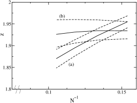
FIG. 3.: The effective dynamic exponent as a function of strip width $N$ at the end points of two FOR line: (a) $(L_{H},L_{V},M_{2},M_{4})=(-0.69,0.69,-0.02,0.02)$ and (b) $(L_{H},L_{V},M_{2},M_{4})=(-0.41,0.69,0.05,-0.05)$. The dashed lines represent the uncertainty in the location of the end points.

FIG. 4.: The ECS near the FRE point in the crossover region between the shapes of Fig. 1 (b) and (c).

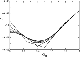
FIG. 5.: The free energy as a function of $Q_{H}$ for $(L_{H},L_{V},M_{2},M_{4})=(0.0,0.69,-0.14,-0.40)$, at $E_{V}=0.683$. Only the $Q_{H}>0$ side is shown. $f(Q_{H})$ is mirror symmetric.

REFERENCES

- [1] For a review, see C. Rottman and M. Wortis, Phys. Rep. 103, 59 (1984).
- [2] See e.g., F. Gallet, S. Balibar, and E. Rolley, Jour. de Phys. 48, 369 (1987).
- [3] J.C. Heyraud and J.J. Métois, Jour. Cryst. Growth 82, 269 (1987).
- [4] T. Ohachi and I. Taniguchi, Jour. Cryst. Growth 65, 84 (1983).
- [5] See L.A.M.J. Jetten, H.J. Human, P. Bennema, and J.P. van der Eerden, Jour. Cryst. Growth 68, 503 (1984) and included references.
- [6] C. Rottman, M. Wortis, J.C. Heyraud, and J.J. Métois, Phys. Rev. Lett. 52, 1009 (1984).
- [7] Y. Carmi, S.G. Lipson, and E. Polturak, Phys. Rev. B 36, 1894 (1987).
- [8] J.C. Heyraud and J.J. Métois, Jour. Cryst. Growth 84, 503 (1987).
- [9] J. Neergaard and M. den Nijs, Phys. Rev. Lett. 74, 730 (1995).
- [10] J.D. Shore and D.J. Bukman, Phys. Rev. Lett. 72, 604 (1994), and Phys. Rev. E 51, 4196 (1995).
- [11] D. Davidson and M. den Nijs, Phys. Rev. E 59, 5029 (1999).
- [12] V.B. Shenoy, S. Zhang, and W.F. Saam, Phys. Rev. Lett. 81, 3475 (1998).
- [13] We do not have enough sensitivity to see the logarithmic factor predicted by S.M. Bhattacharjee, Phys. Rev. Lett. 76, 4568 (1996).
- [14] S. Song and S.G.J. Mochrie, Phys. Rev. Lett. 73, 995 (1994) and Phys. Rev. B 51,10068 (1995).
- [15] M. Lässig, Phys. Rev. Lett. 77, 526 (1996).
- [16] A.F. Andreev, Sov. Phys. JETP 53, 1063 (1981).
- [17] The precise location of these transitions is obscured by modulations in that occur only in this part of the phase diagram. The transition between the rough and tilted rough phases may be partially first-order.