[

Multiscale Random-Walk Algorithm for Simulating Interfacial Pattern Formation

Abstract

We present a novel computational method to simulate accurately a wide range of interfacial patterns whose growth is limited by a large scale diffusion field. To illustrate the computational power of this method, we demonstrate that it can be used to simulate three-dimensional dendritic growth in a previously unreachable range of low undercoolings that is of direct experimental relevance.

]

Interfacial patterns form spontaneously in a wide range of physical and biological systems where the motion of an interface is limited by one (or several) diffusion fields, each one obeying the diffusion equation

$$\partial_{t}u=D\nabla^{2}u$$ (1)

with specified boundary conditions on the interface. Classic examples include various cellular, dendritic, or eutectic solidification patterns (where $u$ represents the temperature or an impurity concentration) [1], dendrite-like branched patterns formed during electrochemical deposition (where $u$ is some ion concentration) [2] and complex growth morphologies produced by bacterial colonies under stress (where $u$ can represent the concentration of some nutrient or a signaling agent) [3].

When attempting to accurately simulate the growth of such structures, one is generally faced with two major difficulties. The first one is front tracking, which requires to resolve accurately the boundary conditions imposed on $u$ at the evolving interface. Dendritic solidification, where even a weak crystalline anisotropy crucially influences the morphological development epitomizes this difficulty. The second problem is the large disparity of scale between the growing structure and the diffusion field surrounding it. The physical origin of this disparity is essentially dimensional. The diffusion field decays ahead of the growth structure on a length scale $l\sim D/v$, where $v$ is the velocity of the advancing interface, whereas the characteristic scale of the structure, e.g. the tip radius $\rho$ of a growing dendrite, is itself the geometric mean of $l$ and a short length scale cutoff proportional to the interface thickness. Thus, for small growth rate, $l$ can be several orders of magnitude larger than $\rho$, and simulations that resolve simultaneously the details of the interfacial pattern and the diffusion field become extremely difficult.

Whereas various methods have been successfully developed to handle front tracking, bridging the length scale gap between $\rho$ and $l$ has remained a major computational challenge. A natural idea to overcome this problem is to use multigrid or adaptive mesh refinement algorithms that make the grid progressively coarser away from the interface [4, 5, 6]. However, such methods need to dynamically adapt their grids to follow the moving interface. This is a nontrivial task, and quantitative simulations of dendritic crystal growth at low undercooling have remained restricted to two dimensions (2-d) [6].

In this letter, we present a novel hybrid computational approach that efficiently bridges this length scale gap. Over most of the computational domain, the diffusion equation is simulated by an ensemble of off-lattice random walkers that take longer, and concomitantly rarer, steps with increasing distance away from the growing interface. This drastically reduces the computational cost for evolving the large-scale field. Moreover, a short distance away from the interface, this stochastic evolution is connected to a finite-difference deterministic solution of the interface evolution. This conversion, in turn, reduces the inherent noise of the stochastic method to a negligibly small level at the interface. This approach is relatively simple to implement in both 2-d and 3-d while being at the same time quantitatively accurate. Here we sketch the method and then report results that demonstrate its capability to yield new quantitative predictions testable by experiments in the context of dendritic crystal growth. For clarity, we expose the method in this context although it will become clear below that it is general.

Let us consider a solid-liquid interface whose motion is limited by heat diffusion and define a scaled temperature field $u$ that is zero in equilibrium and equal to $-\Delta$ in the liquid far from the interface, where $\Delta$ is the dimensionless undercooling. At the interface, $u$ satisfies the well-known boundary conditions

$$v_{n} = D\left(\left.\partial_{n}u\right|_{s}-\left.\partial_{n}u\right|_{l}\right),$$ (2)

$$u = -d_{0}\sum_{i=1}^{2}\left[a({\hat{n}})+\partial_{\theta_{i}}^{2}a({\hat{n}})\right]\kappa_{i},$$ (3)

corresponding to heat conservation and local thermodynamic equilibrium at the interface, respectively, where $v_{n}$ is the normal velocity of the interface, $d_{0}$ is a microscopic capillary length, $\theta_{i}$ are the local angles between the normal $\hat{n}$ to the interface and the two local principal directions on the interface, $\kappa_{i}$ are the principal curvatures, and the function $a(\hat{n})$ describes the orientation dependence of the surface energy.

The basic idea of the method is to divide space into an ‘inner’ and an ‘outer’ domain as illustrated in Fig. 1. The inner domain consists of the growing structure and a thin ‘buffer layer’ of liquid surrounding the interface. The outer domain corresponds to the rest of the liquid, and is much larger than the inner domain at low undercooling. In the inner domain, we solve deterministically the diffusion equation on a fine uniform mesh. Moreover, for the present crystal growth application, we handle front tracking using a phase-field approach [7], and time-step explicitly both $u$ and the phase-field in the inner region using the same procedure as Karma and Rappel [8]. The geometry of Fig. 1, however, implies that any other front tracking method that solves the diffusion equation on a uniform mesh could be used instead. Moreover, since the boundary conditions on $u$ need not necessarily be those defined by Eqs. 2 and 3, the method obviously extends to other diffusion-limited pattern forming systems.

In the outer domain, the diffusion equation is simulated stochastically by an ensemble of off-lattice random walkers. The idea of solving the diffusion or Laplace equation with an ensemble of random walkers is well-known and has been used previously to simulate diffusion-limited growth [9] and Hele-Shaw flow [10]. The main new feature of our method is that we have separated the solid-liquid interface from the boundary at which the conversion from the deterministic to the stochastic solution of the diffusion equation takes place. This separation yields two essential benefits. Firstly, it makes it possible to use the phase-field approach with its proven accuracy to simulate the interface evolution and to resolve even a weak crystalline anisotropy, without being affected by the details of the conversion process. Secondly, in the buffer layer between the solid-liquid interface and the conversion boundary, the temperature obeys the deterministic diffusion equation. Consequently, the noise created by the stochastic release and impingement of walkers is rapidly damped away from the conversion boundary. Hence, the amplitude of temperature fluctuations at the solid-liquid interface can be reduced to an insignificant level without much cost in computation time by increasing the thickness of the buffer layer.

To connect the inner (deterministic) and outer (stochastic) solutions, we have to supply a boundary condition for the integration of the inner region, and we must specify how walkers are created and absorbed at the boundary between inner and outer regions. Both processes are handled by using a coarse-grained grid that is superimposed on the fine grid of the inner region as shown in Fig. 1. Cells of the coarse grid on the border between inner and outer region, shaded in Fig. 1, are called conversion cells. The temperature in a conversion cell is related to the local density of walkers,

$$u_{cc}=-\Delta\left(1-{m_{i}(t)/M}\right),$$ (4)

where $m_{i}(t)$ is the number of walkers in conversion cell number $i$ at time $t$, and $M\gg 1$ is a fixed integer. Hence, an empty cell corresponds to $u=-\Delta$ (the initial state), whereas a box containing $M$ walkers corresponds to $u=0$. This formula is used in each timestep to obtain the boundary condition for the integration of the inner region. Next, we determine the quantity of heat that flows in or out of each conversion cell from the inner region, and add this amount to a reservoir variable $H_{i}(t)$ which describes the heat content of conversion cell number $i$. If this variable exceeds a critical value $H_{c}$, a walker is created and $H_{c}$ is subtracted from the reservoir. Conversely, if $H_{i}(t)$ falls below $-H_{c}$, a walker is absorbed and $H_{c}$ is added to the reservoir. This procedure assures that walkers are created and absorbed at a rate which is proportional to the local heat flux, and each walker corresponds to the same discrete amount of heat.

FIG. 1.: Top: snapshot of a 2-d simulation for $\Delta=0.1$ and $\epsilon_{4}=0.025$ showing the solid-liquid interface (solid line), the inner-outer domain conversion boundary (dashed-line), and the random walkers (dots). Only a small part of the outer domain and one out of 50 walkers are shown for clarity. Bottom: enlarged view of the conversion boundary (dashed line) showing the fine and coarse grids. Shaded cells are conversion cells and walkers (dots) are restricted to the outer region.

Evidently, as the structure grows the geometry of the conversion boundary and the configuration of the coarse grid need to be periodically updated in order to maintain a constant thickness of the liquid buffer layer. This procedure, however, is straightforward since the structure of the grids does not change.

In the outer region, each walker is represented by a set of variables indicating its position and the time it has next to be updated. To update a walker, a new position is randomly selected with a probability distribution given by the diffusion kernel,

$$P(\vec{x}^{\prime},t^{\prime}|\vec{x},t)=\frac{1}{\left[4\pi D(t^{\prime}-t)\right]^{d/2}}\exp-{{|\vec{x}^{\prime}-\vec{x}|}^{2}\over 4D(t^{\prime}-t)},$$ (5)

where $\vec{x}$ and $\vec{x}^{\prime}$ are the old and new positions of the walker, respectively, and $t^{\prime}-t$ is the time increment between updates. This representation of the diffusion equation is widely used in quantum Monte Carlo methods [11]. The key improvement that makes the algorithm efficient in the present context is the introduction of a variable step size: we allow walkers to take progressively larger steps with increasing distance away from the interface, and to be concomitantly updated more rarely, which does not affect the quality of the solution near the solid-liquid interface. Adaptive steps have been previously used to speed up simulations of diffusion-limited aggregation, albeit in a simpler Laplacian context where the stepping time is irrelevant and only one walker at a time is simulated [12]. Typically, we vary the average step size between a value comparable to the spacing of the inner mesh to about $100$ times that value. Our test dendrite computations show that the far field can be evolved at essentially no extra cost: the program spends most of its time in the inner region and for the walkers which are near to the conversion boundary and have to make small steps. Thus this ‘adaptive step’ implementation yields essentially the same benefits as an adaptive meshing algorithm, while avoiding the overhead of regridding. Finally, our method can be easily parallelized as will be discussed in more details elsewhere.

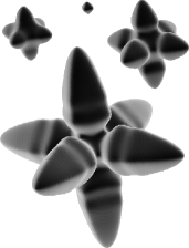
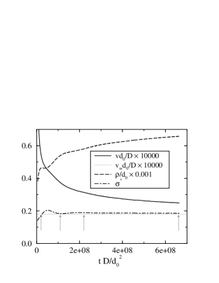
FIG. 2.: Result of a 3-d dendrite growth simulation for $\Delta=0.05$ and $\epsilon_{4}=0.025$ with snapshots of the 3-d structure (top) at the times corresponding to the arrows. This run took 6 hours on 64 processors of the CRAY T3E at NERSC and used up to $5\times 10^{6}$ walkers.

To illustrate our method, we focus here on the initial stage of dendritic solidification, during which four (six) primary arms in 2-d (3-d) emerge from a structureless nucleus, as shown in the example 3-d run of Fig. 2. While this transient regime has recently been investigated numerically in 2-d and experimentally in 3-d [13], it has not yet been explored by simulations in 3-d.

The present simulations started from a small spherical solid nucleus with a uniformly undercooled temperature $u=-\Delta$, and fully exploited a cubic symmetry (i.e. $a(\hat{n})\equiv(1-3\epsilon_{4})[1-4\epsilon_{4}/(1-3\epsilon_{4})(n_{x}^{4}+n_{y}^{4}+n_{z}^{4})]$ with the Cartesian axes defined parallel to the [100] directions) to reduce simulation time. The value $\epsilon_{4}=0.025$ that corresponds to the experimentally estimated anisotropy value for pivalic acid (PVA) [14] was used in all the simulations reported here. Results for other anisotropies and that pertain to the 3-d morphology of the dendrite tip will be discussed elsewhere. To obtain quantitative data on the growth transients, we recorded the arm length $L(t)$, the tip velocity $v(t)=\dot{L}(t)$, the tip radius of curvature $\rho(t)$, and the total volume of solid $V_{s}(t)$. In Fig. 2, we show $v(t)$ and $\rho(t)$ for a 3-d run at $\Delta=0.05$ together with the time-dependent tip selection parameter $\sigma^{*}(t)=2d_{0}D/[\rho^{2}(t)v(t)]$ and the steady-state velocity $v_{ss}$ calculated by a boundary integral method. Two results are particularly noteworthy. Firstly, $\sigma^{*}(t)$ becomes essentially constant as soon as the arms have emerged from the spherical seed, whereas both $v(t)$ and $\rho(t)$ are far from their steady-state values. Physically, this is a direct consequence of the fact that $v(t)$ and $\rho(t)$ evolve slowly on the tip diffusion time scale $\rho^{2}/D$ where $\sigma^{*}$ is established. Secondly, we find that, as the undercooling is lowered, the volume of the dendrite (or its area in 2-d) approaches that of a sphere (circle) growing at the same undercooling. The latter is readily obtained from Zener’s well-known similarity solution, which yields that the radius of a $d$-dimensional sphere grows as $\sqrt{4p_{d}Dt}$, where the Peclet number $p_{d}(\Delta)$ is implicitly defined by $\Delta=p_{d}^{d/2}\exp(p_{d})\int_{p_{d}}^{\infty}s^{-d/2}e^{-s}ds$. Both in 2-d and 3-d, the volume of the dendrite grows slightly faster than the one of the sphere, but for the lowest undercoolings we could attain, the final volume differed by only $20\%$ from this prediction, even though the arms were already very well developed.

The above observations are in good agreement with theoretical expectations for 2-d growth transients. In particular, Almgren et al. have analyzed the related problem of anisotropic Hele-Shaw flow (i.e. Laplacian growth) at constant flux [15]. Using an exact solution for the Laplacian field around a cross and exploiting the constancy of $\sigma^{*}$, they constructed a self-affine scaling shape for the arms. The length and width of this shape grows as $t^{\alpha}$ and $t^{\beta}$, respectively, with $\alpha=3/5$ and $\beta=2/5$. As subsequently remarked by Brener [16], the diffusion equation can be replaced by Laplace’s equation on the scale of the dendrite as long as $L/\sqrt{Dt}\ll 1$, and hence 2-d growth transients should obey this scaling with a flux set by the diffusive far field of Zener’s similarity solution in the low undercooling limit. In Fig. 3a, we plot the functions $\alpha(t)=d(\ln L)/d(\ln t)$ and $\nu(t)=d(\ln V_{s})/d(\ln t)$. For an exact Laplacian scaling in 2-d, $\alpha(t)=3/5$ and $\nu(t)=1$. With decreasing undercooling both curves become flatter and indeed approach the expected Laplacian scaling. The slow rise with time of both curves can be attributed to diffusive corrections to the Laplacian scaling due to the slow increase in time of $L/\sqrt{Dt}$. Recently, Provatas et al. have reported scaling exponents that differ from the Laplacian prediction and that appear to be independent of $\Delta$ for small $\Delta$ [13]. We note, however, that they used the distance from the tip to the time-dependent base (where the dendrite shaft is narrowest) to scale their results instead of $L(t)$. Since $L(t)$ is the only relevant scaling length for both the shape and the diffusion field in the Laplacian limit, we believe that these exponents are spurious. When $L(t)$ is used as a scaling length, our results are consistent with an approach to Laplacian scaling in the limit of vanishing undercooling.

It is simple to heuristically generalize some of the above ideas to 3-d. If we assume, as a reasonable first approximation, that the arm shape is axisymmetric and has a scaling form $r(x,t)=t^{\beta}\tilde{r}\left(x/t^{\alpha}\right)$, where $x$ is the growth direction, the constancy of $\sigma^{*}$ imposes that $4\beta-\alpha-1=0$. Furthermore, assuming that the volume of the dendrite grows approximately as the one of the 3-d similarity solution, we have in addition $\nu=\alpha+2\beta=3/2$. These two conditions yield $\alpha=2/3$ and $\beta=5/12$. Fig. 3b shows the functions $\alpha(t)$ and $\nu(t)$, defined as before, in 3-d. As in 2-d, the curves approach the predicted exponents with decreasing undercooling, but the differences remain larger than in 2-d even for the lowest undercooling. This can be partly accounted for by the fact that the tip velocity, and hence also $L/\sqrt{Dt}$, is much larger in 3-d than in 2-d at equal undercoolings. We must emphasize that in the absence of an exact 3-d Laplacian solution, and in view of the above assumptions, no claim is made here that these 3-d exponents are exact or that a scaling regime exists asymptotically at small undercooling in 3-d. We content ourselves with the fact that they describe reasonably well our present simulations.

In conclusion, we have presented a novel computational approach that can resolve accurately the details of a complex branched structure and its large scale surrounding diffusion field. The method can be combined with many of the existing front tracking methods and should be applicable to a wide range of diffusion-limited pattern forming systems. Furthermore, we have demonstrated its feasibility in the non-trivial test case of dendritic growth in a range of parameters previously unreachable in 3-d.

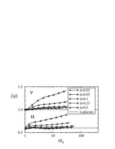
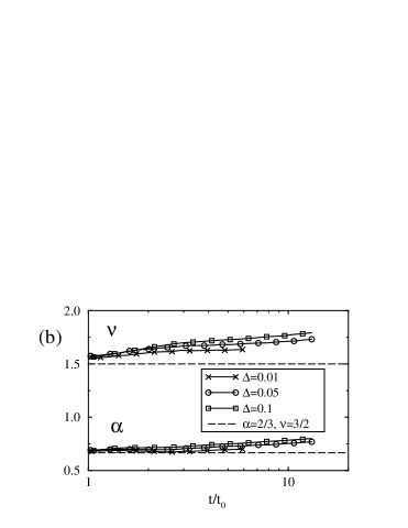
FIG. 3.: Functions $\alpha(t)$ and $\nu(t)$ vs scaled time $t/t_{0}(\Delta)$ in 2-d (a) and 3-d (b). In order to show all curves on the same plot, $t_{0}(\Delta)$ was defined to be the time at which the tips are ahead of the grooves by about two tip radii. In order of decreasing $\Delta$, $t_{0}D/d_{0}^{2}=2.29\times 10^{4}$, $9.03\times 10^{5}$, $4.36\times 10^{7}$, $5.35\times 10^{8}$, and $1.39\times 10^{10}$ in 2-d, and $4.18\times 10^{6}$, $5.58\times 10^{7}$ and, $1.17\times 10^{10}$ in 3-d.

This research is supported by U.S. DOE Grant No. DE-FG02-92ER45471 and benefited from computer time allocation at NERSC and NU-ASCC. We thank Flavio Fenton for help with 3-d visualization of our simulations and Vincent Hakim for fruitful conversations.

REFERENCES

- [1] W. Kurz and D. J. Fisher, Fundamentals of solidification (Trans Tech, Aedermannsdorf, Switzerland, 1992).
- [2] M. Matsushita, M. Sano, Y. Hayakawa, H. Honjo, and Y. Sawada, Phys. Rev. Lett. 53, 286 (1984).
- [3] E. Ben-Jacob, H. Shmueli, O. Shochet, and A. Tenenbaum, Physica A 187, 378 (1992).
- [4] A. Schmidt, J. Comp. Phys. 125, 293-312 (1996).
- [5] R. J. Braun and M. T. Murray, J. Cryst. Growth 174, 41 (1997)
- [6] N. Provatas, N. Goldenfeld, and J. Dantzig, Phys. Rev. Lett. 80, 3308 (1998); J. Comp. Phys. 148, 265 (1999).
- [7] J. S. Langer, in Directions in Condensed Matter, ed. by G. Grinstein and G. Mazenko (World Scientific, Singapore, 1986), p. 164; J. B. Collins and H. Levine, Phys. Rev. B 31, 6119 (1985).
- [8] A. Karma and W.-J. Rappel, Phys. Rev. E57, 4323 (1998).
- [9] T. Vicsek, Phys. Rev. Lett. 53, 2281 (1984).
- [10] L. P. Kadanoff, J. Stat. Phys. 39, 267 (1985); S. Liang, Phys. Rev. A 33, 2663 (1986).
- [11] See for example S. E. Koonin and D. C. Meredith, Computational Physics (Addison-Wesley, Redwood City, 1992).
- [12] P. Meakin, Phys. Rev. A 27, 1495 (1983).
- [13] N. Provatas et al., Phys. Rev. Lett. 82, 4496 (1999).
- [14] M. Muschol, D. Liu, and H. Z. Cummins, Phys. Rev. A 46, 1038 (1992).
- [15] R. Almgren, W.-S. Dai, and V. Hakim, Phys. Rev. Lett. 71, 3461 (1993).
- [16] E. Brener, Phys. Rev. Lett. 71, 3653 (1993).