Phase Diagram of the Lattice Restricted Primitive Model

Abstract

We present a comprehensive study of the lattice restricted primitive model, i.e., a lattice gas consisting of an equal number of positively and negatively charged particles interacting via on-site exclusion and a $1/r$ potential. On the cubic lattice, Monte Carlo simulations show a line of Néel points separating a disordered, high-temperature phase from a phase with global antiferromagnetic order. At low temperatures the (high-density) ordered phase coexists with the (low-density) disordered phase. The Néel line meets the coexistence curve at a tricritical point, $T_{t}\simeq 0.14$, $\rho_{t}\simeq 0.4$. A simple mean-field analysis is in qualitative agreement with simulations.

Introduction

It has long been realized that the presence of an appreciable concentration of free ions in a system of overall charge neutrality gives rise to a variety of thermodynamic features not found in un-ionized systems. For example, in the restricted primitive model (RPM), a system of charged hard-sphere anions and cations, all with equal charge magnitude $|q|$ and diameter $\sigma$, one has the famous limiting law established by the work of Debye and Hückel dhxx in 1923,

$$-\frac{A^{ex}}{k_{B}TV}\rightarrow\frac{\Gamma_{D}^{3}}{12\pi}\;\;\;\mbox{ as }\;\;\rho\rightarrow 0,\;\;T\;\;\mbox{fixed}.$$ (1)

Here $A^{ex}$ is the Helmholtz free energy (excess to the ideal-gas condition), $V$ is the system volume, $k_{B}$ Boltzmann’s constant, $T$ the temperature, $\rho$ the total number density of anions and cations, and $\Gamma_{D}$ is the inverse Debye length, $\Gamma_{D}^{2}\sigma^{2}=4\pi\rho q^{2}/k_{B}T$. This is in marked contrast to an un-ionized fluid, for which $A^{ex}/k_{B}TV$ approaches a second virial-coefficient term proportional to $\rho^{2}$ rather than $\rho^{3/2}$.

Results pertaining to phase transitions and criticality in the RPM did not emerge until much after the work of Debye and Hückel. It was not until 1976 that a systematic study by Stell, Wu, and Larsen appeared with the conclusion that the RPM should exhibit a liquid-gas coexistence curve with a critical point swl76 . They further concluded that the critical density is much lower than for a simple argon-like fluid model, but found that that the shape and location of the coexistence curve was very sensitive to the details of the approximations that must inevitably be used in such a theoretical study. Monte Carlo simulations have yielded results fully consistent with their conclusions, but only in the last few years have the studies of different groups converged toward common values for the critical density and temperature of the RPM orkoulas ; caillol ; valleau .

As one of us has discussed in earlier studies stell92 ; stell95 , the RPM can be thought of as a spin system with a long-ranged antiferromagnetic interaction

$$J(r)=-\frac{q^{2}}{r\epsilon},$$ (2)

and one-dimensional spins ${\bf s}_{i}$ with $|{\bf s}_{i}|=1$;

$$\phi_{ij}(r)=-J(r){\bf s}_{i}\cdot{\bf s}_{j}\;.$$ (3)

(Since the “spins” are charges, we should perhaps refer to the interaction as antiferroelectric rather than antiferromagnetic.) The lattice-gas version of such a spin fluid is simply the spin-1 Ising model with $|{\bf s}|=1$, 0, or -1, with ${\bf s}=0$ representing a vacant site. We shall refer to this model, which forms the subject of this report, as the lattice restricted primitive model (LRPM).

For a lattice gas with a nearest-neighbor $J({\bf r})$ instead of a Coulombic $J({\bf r})$, the spin-1 Ising model is a Blume-Capel model blume ; capel , which becomes equivalent, at full occupancy, to a nearest-neighbor spin-$\onehalf$ Ising model that is exactly-soluble on many two-dimensional lattices mccoy ; baxter . On the square lattice one finds a Néel point as one lowers the temperature in the absence of an external field. Moreover, although exact results are lacking in three dimensions, one expects for bipartite lattices such as the simple cubic, that as one lowers the density along the $\lambda$-line of Néel points in the $\rho$-$T$ plane, one encounters a tricritical point below which the lattice gas phase-separates into paramagnetic and antiferromagnetic phases. This immediately raises the question whether this remains true for a lattice gas with a Coulombic $J({\bf r})$.

Several years ago, in order to better understand the LRPM, we initiated Monte Carlo simulations on a simple cubic lattice. Our results are fully consistent with the presence of a $\lambda$-line of Néel points terminating in a tricritical point, below which (in $T$) two phases coexist. Preliminary results were reported in Ref. stell99 ; here we provide more extensive results as well as details of our simulation procedure. We have supplemented our simulations with a mean-field analysis that exploits the similarity between the LRPM and a nearest-neighbor lattice gas. Høye and Stell hs97 have also made a more general study of the spin-1 Ising model that included the solution of the mean-spherical approximation (MSA) for a range-parametrized $J({\bf r})$. As discussed by these authors, the MSA is not appropriate to study criticality and phase separation in the spin-1 model with Coulombic $J({\bf r})$ (although, as they show, it does yield the correct Debye-Hückel limiting law). The Høye-Stell study, however, goes beyond the MSA with a number of general observations that strongly support tricriticality for a Coulombic $J({\bf r})$.

More recent studies made by Ciach and Stell ciach of ionic models that include the continuum-space and lattice RPM reveal that generically such models can be expected to manifest criticality, tricriticality, or both, depending upon the precise forn of their Hamiltonians. For example, the work suggests that some extended-core lattice models may well show both liquid-gas like criticality and, at higher densities, a $\lambda$-line with associated tricriticality. For the RPM, the critical properties that follow from application of RG analysis are found to be in the Ising universality class.

Model

We consider a lattice gas of particles interacting via site exclusion (multiple occupancy forbidden) and a Coulomb interaction $u(r_{ij})=s_{i}s_{j}/r_{ij}$, where $r_{ij}=|{\bf r}_{i}-{\bf r}_{j}|$ is the distance separating the particles (located at lattice sites ${\bf r}_{i}$ and ${\bf r}_{j}$), and $s_{i}=+1$ or $-1$ is the charge of particle $i$. Exactly half the $N$ particles are positively charged; the remainder are negative. They are restricted to a simple cubic lattice of $V=L^{3}$ sites, with periodic boundaries. We assume a lattice constant $a$ of unity, and adopt units in which $q^{2}/ak_{B}=1$, $q$ being the magnitude of the charge. In what follows we treat charge, length, energy and temperature as dimensionless.

We note in passing that in lattice simulations of ionic systems an alternative definition of the potential is possible, i.e., $u({\bf r}_{ij})=s_{i}s_{j}\Phi({\bf r}_{ij})$, where $\Phi$ is the Green’s function for Poisson’s equation on the lattice in question. While the simple $1/r$ potential and the lattice Green’s function differ somewhat at short distances, they have the same asymptotic (large $r$) behavior, and we expect (qualitatively) the same phase diagram in either case.

In this study we restrict attention to the simple cubic lattice. This lattice, like the body-centered cubic, admits a decomposition into two sublattices (the sites on one sublattice having all nearest neighbors in the other sublattice), which obviously facilitates formation of an ordered state resembling an ionic crystal. Indeed, it was proven some time ago that the LRPM on the simple cubic lattice exhibits long-range order at sufficiently low temperatures and high fugacities lieb80 . The model presents, as we will show, a strong tendency to assume a NaCl-like ordered state at low temperatures. It would be interesting to study the model on the face-centered cubic lattice or another structure that frustrates antiferromagnetic ordering.

Mean-Field Analysis

The energy of the lattice restricted primitive model is

$$U=\frac{1}{2}\sum_{i,j}\frac{s_{i}s_{j}}{r_{ij}},$$ (4)

where it is understood that the particles occupy distinct lattice sites. We consider the LRPM with independent variables $T$ (temperature) and $\rho\equiv N/V$. It is helpful to think of this system as a three-state (i.e., spin-1) antiferromagnetic Ising model with long-range interactions ($J\sim 1/r$). On a fully occupied lattice ($\rho=1$) we characterize ordering by the sublattice charge disparity or staggered magnetization $\phi$. In the context of MFT, this allows us to replace Eq. (4) by the corresponding expression for a nearest-neighbor (NN) lattice gas, multiplied by a suitable factor.

Consider first the disordered system. Since the neighbors of any given particle are equally likely to bear the same or opposite charges, the mean-field estimate for the energy is zero, just as for the NN system. Next, suppose there is sublattice ordering; let $\rho_{+}^{A}$ be the fraction of sites in sublattice $A$ occupied by positive particles, etc., and let

$$\rho_{+}^{A}=\frac{\rho}{2}(1+\phi)\;;\;\;\;\;\;\;\;\rho_{+}^{B}=\frac{\rho}{2}(1-\phi)$$ (5)

$$\rho_{-}^{A}=\frac{\rho}{2}(1-\phi)\;;\;\;\;\;\;\;\;\rho_{-}^{B}=\frac{\rho}{2}(1+\phi),$$ (6)

so that

$$\phi=\frac{\rho_{+}^{A}-\rho_{-}^{A}}{\rho},$$ (7)

and

$$\rho_{+}^{A}+\rho_{-}^{A}=\rho_{+}^{B}+\rho_{-}^{B}=\rho.$$ (8)

Using these, the mean-field estimate for the energy of a pair of nearest-neighbor sites is

$$u_{NN} = \rho_{+}^{A}\rho_{+}^{B}+\rho_{-}^{A}\rho_{-}^{B}-\rho_{+}^{A}\rho_{-}^{B}-\rho_{-}^{A}\rho_{+}^{B}$$ (9)

$$= -\rho^{2}\phi^{2}.$$

Similarly, the MF estimate for the energy of a pair of second-neighbor sites (which must belong to the same sublattice) is $+\rho^{2}\phi^{2}/\sqrt{2}$, and so on. Thus MFT gives the energy of the LRPM as

$$U_{MF}=\frac{\rho^{2}\phi^{2}}{2}\sum_{i,j}\frac{(-1)^{S}}{r_{ij}},$$ (10)

where $S=+1(-1)$ if sites $i$ and $j$ belong to the same (different) sublattices. The sum (including the factor of 1/2) is simply the electrostatic energy of an ionic crystal. For the simple cubic lattice,

$$\frac{1}{2}\sum_{i,j}\frac{(-1)^{S}}{r_{ij}}=-3V\frac{\alpha}{6},$$ (11)

as $V\rightarrow\infty$, where $\alpha=1.7457$ is the Madelung constant tosi . Thus the mean-field energy per site is $u_{MF}=-\alpha\rho^{2}\phi^{2}/2$, while the corresponding expression for a system with nearest-neighbor interactions is $-3\rho^{2}\phi^{2}$. In the context of MFT, then, we may replace the $1/r$ potential with a nearest-neighbor interaction.

From the preceding analysis it appears that we may treat the LRPM, in MFT, as if it were a nearest-neighbor lattice gas, but with an energy (and temperature) scale that is smaller by a factor of $\alpha/6\simeq 0.2913$. A more meaningful way of relating the temperature scales, however, is to compare the energy change attending an elementary excitation, in this case, the interchange of a nearest-neighbor pair in a perfectly ordered lattice. In the simple cubic lattice this raises the energy by $\Delta U_{NN}=20$ (the nearest-neighbor interaction $J=1$), since ten nearest-neighbor pairs have like charges after the exchange. For the ionic crystal (NaCl structure) the corresponding energy change is $4(\alpha-1)\simeq 2.9903$, so that $\Delta U_{LRPM}\simeq 0.1495\Delta U_{NN}$. Since the mean-field critical temperature for the (fully occupied) nearest-neighbor lattice gas is 6 on the cubic lattice, the corresponding result for the LRPM is about 0.9. The best numerical estimate for the lattice gas is $T_{c}=4.5115$; the corresponding LRPM value is 0.674. (Extrapolation of our simulation results to $\rho=1$ yields $T_{c}\approx 0.6$.)

We may now develop the MFT of the LRPM by studying the nearest-neighbor lattice gas, bearing in mind the difference in temperature scales explained above. To estimate the entropy as a function of $\rho$ and $\phi$, we note that the number of allowed configurations on a sublattice of $V/2$ sites is $(V/2)!/[N_{+}!N_{-}!N_{v}!]$ where $N_{+}$ ($N_{-}$) is the number of positive (negative) particles and $N_{v}=[(V/2)-N_{+}-N_{-}]$ the number of vacant sites on the sublattice. Using $N_{\pm}=(1\pm\phi)\rho V/4$, etc., and Stirling’s formula, we obtain the entropy per site,

$$s=-\rho\ln\rho-(1\!-\!\rho)\ln(1\!-\!\rho)+\rho\ln 2-\frac{\rho}{2}[(1+\phi)\ln(1+\phi)+(1-\phi)\ln(1-\phi)]\;.$$ (12)

Let $f=u-Ts$ be the Helmholtz free energy per site. To investigate the possibility of a free energy minimum with nonzero sublattice ordering $\phi$, we note that

$$\left(\frac{\partial f}{\partial\phi}\right)_{\rho}=\rho\left[-6\rho\phi+\frac{T}{2}\ln\frac{1+\phi}{1-\phi}\right]\;.$$ (13)

A free energy minimum therefore implies that

$$\frac{12\rho\phi}{T}=\ln\frac{1+\phi}{1-\phi}\;.$$ (14)

Expanding the r.h.s. as $2\phi+2\phi^{3}/3+\cdots$, we see that solutions with nonzero $\phi$ exist for $T<T_{c}=6$ and $\rho>\rho_{c}=T/T_{c}$. For $\rho\stackrel{{\scriptstyle>}}{{\sim}}\rho_{c}$,

$$x\simeq\pm\sqrt{3\left[\frac{\rho}{\rho_{c}}-1\right]}\;.$$ (15)

Thus $T=6\rho$ is a line of second-order phase transitions (a Néel or lambda line), separating the high-temperature phase ($x=0$) from one with sublattice ordering.

Next we investigate the stability of the uniform-density state. Defining $f_{p}=f/\rho$ as the free energy per particle, we may write the chemical potential as

$$\mu=f_{p}+\frac{p}{\rho}\;,$$ (16)

where the pressure $p$ is given by

$$p=\rho^{2}\left(\frac{\partial f_{p}}{\partial\rho}\right)_{T}=-T\ln(1-\rho)-3\rho^{2}\phi^{2}\;.$$ (17)

(In evaluating the derivative we use Eq. (14) to eliminate $(\partial\phi/\partial\rho)_{T}$.) The pressure in the disordered phase is that of a simple lattice gas; but for $T<T_{c}$, $(\partial p/\partial\rho)_{T}$ suffers a discontinuity at $\rho_{c}$. Using Eq. (15) we have that for $\rho\stackrel{{\scriptstyle>}}{{\sim}}\rho_{c}$,

$$\left(\frac{\partial p}{\partial\rho}\right)_{T}=\frac{T}{1-\rho}-9\rho\left(\frac{3\rho}{\rho_{c}}-2\right)\;,$$ (18)

so that

$$\left(\frac{\partial p}{\partial\rho}\right)_{T;\rho=\rho_{c}}=T\left(\frac{1}{1-\rho_{c}}-\frac{3}{2}\right)\;.$$ (19)

Thus the inverse compressibility vanishes when $\rho_{c}=1/3$, which implies $T=2$. This marks a tricritical point, at which the Néel line meets the coexistence curve. (For $T<2$ the extension of the Néel line, $T=6\rho$, is in fact a spinodal.) Recalling the temperature rescaling, our MFT gives a tricitical temperature of 0.3 for the LRPM, or $T_{t}=0.225$ if we use the best estimate ($T_{c}=4.5115$) in place of the mean-field result ($T_{c}=6$) for the simple lattice gas. Typical pressure-density curves are shown in Figure 1.

Figure 1: Mean-field theory predictions for the pressure versus density at temperatures 0.449 (upper curve), $T_{t}=0.299$ (middle), and 0.224 (lower).

Figure 2: Mean-field prediction for the phase diagram of the LRPM.

We construct the coexistence curve by finding the densities $\rho_{1}$ and $\rho_{2}$ for which $p(\rho_{1},T)=p(\rho_{2},T)$ and $\mu(\rho_{1},T)=\mu(\rho_{2},T)$. This is done numerically, through an iterative procedure. A first guess for $\rho_{2}$ is the mean of $\rho_{s}^{+}$ (the high-density spinodal, found by setting the r.h.s. of Eq.(18) to zero), and $\rho_{m}$, the density at which the pressure equals $p(\rho_{s}^{-})$, its value on the low-density spinodal. A first guess for $\rho_{1}$ is the density at which $p(\rho_{1})=p(\rho_{m})$, given by the low-density isotherm, $\rho=1-e^{-p/T}$. We then compare chemical potentials; if $\mu(\rho_{2})>\mu(\rho_{1})$, our guess for $\rho_{2}$ lies above the coexistence value, and vice-versa. By refining the estimate for $\rho_{2}$, recalculating $\rho_{1}$, and repeating the comparison, we rapidly converge on the coexisting densities. For temperatures $T\leq 0.5$ one may use $\phi=1-2e^{-12\rho_{2}/T}\simeq 1$ to show that $\rho_{2}\simeq 1-e^{-3/T}$ and $\rho_{1}\simeq 2e^{-3\rho_{2}/T}$. The mean-field phase diagram for the LRPM (with temperature scaled such that $T_{t}=0.3$) is shown in Figure 2.

Simulation Methods

Electrostatic energy of a periodic array

This subsection presents the multipole expansion as an efficient alternative to Ewald summation for evaluating the electrostatic energy of a periodic array of point charges. Our approach is closely related to the one employed by Ladd in simulations of ionic and dipolar fluids ladd . We require the electrostatic energy of an infinite, periodic array of cells containing point charges. Each cell harbors $N/2$ positive charges and and equal number of negative charges; the position of particle $i$ in cell $j$ is

$${\bf x}_{i,j}={\bf x}_{i}+{\bf R}_{j}\;,$$ (20)

where x_i is the position in the central cell, and

$${\bf R}_{j}=a(n_{x}\hat{\bf x}+n_{y}\hat{\bf y}+n_{z}\hat{\bf z}),$$ (21)

where $n_{\alpha}$ may assume any integer value. (The cell structure is that of a simple cubic lattice; the positions x_i may or may not be restricted to a lattice.)

We write the electrostatic energy of the array as $U=(1/2)\sum_{i=1}^{N}q_{i}\Phi_{i}$, where $\Phi_{\rm i}$ is the potential at the position of charge i. When calculating $\Phi_{i}$ we consider a cube of side $a$ (oriented parallel to the periodic array), centered on charge $i$, and write

$$\Phi_{i}=\Phi_{i,0}+\Phi_{i,a},$$ (22)

where $\Phi_{i,0}$ is the contribution from the charges (other than i) within the cube, and $\Phi_{i,a}$ is the potential at the center of the cube (i.e., the position of charge i) due to the infinite collection of periodic image cells. (These cells include the image of charge $i$, as they must, if they are to be neutral.) The lattice sum defining $\Phi_{i,a}$ is conditionally convergent, and is often treated using the Ewald technique deleeuw . Here, however, we evaluate $\Phi_{i,a}$ via a multipole expansion. The contribution to $\Phi_{i,a}$ due to cell $j$ ($j$ is a shorthand for the cell indices $n_{x}$, $n_{y}$, and $n_{z}$), is

$$\Phi_{i,j}=4\pi\sum_{l,m}\frac{q_{lm}}{2l+1}\frac{Y_{lm}(\theta_{j},\phi_{j})}{R_{j}^{l+1}}.$$ (23)

Here $Y_{lm}$ is the spherical harmonic, $R_{j}=a\sqrt{n_{x}^{2}+n_{y}^{2}+n_{z}^{2}}$, $\cos\theta_{j}=an_{z}/R_{j}$, $\tan\phi_{j}=n_{y}/n_{x}$, and

$$q_{l,m}=\sum_{i=1}^{N}q_{i}r_{i}^{l}Y_{lm}^{*}(\theta_{i},\phi_{i}),$$ (24)

is the $(l,m)$ multipole moment of (any) cell, with $(r_{i},\theta_{i},\phi_{i})$ denoting the position of particle $i$ relative to a convenient origin, for example the cell center. (The monopole moment $q_{00}$ vanishes by charge-neutrality.)

Summing the contributions from all cells (except the central one) yields

$$\Phi_{i,a}=4\pi\sum_{l,m}\frac{q_{lm}}{2l+1}\sum_{j}\frac{Y_{lm}(\theta_{j},\phi_{j})}{R_{j}^{l+1}},$$ (25)

where the sum on $j$ stands for a sum on $n_{x}$, $n_{y}$, and $n_{z}$ (not all zero). This sum over cells is independent of the charge distribution (which appears only in the $q_{lm}$), and so need only be evaluated once. Many terms vanish by symmetry. Thus all terms with $l$ odd are zero since $Y_{lm}$ is then an odd function of $\cos\theta$, while the distribution of cells in the cubic lattice is symmetric about $\theta=\pi$. Symmetry also implies that nonzero contributions have $m=4n$ ($n$ integer), since for each cell with azimuthal angle $\phi$, there are corresponding cells with angles $\phi+\pi/2$, $\phi+\pi$, and $\phi+3\pi/2$, and $1+e^{im\pi/2}+e^{im\pi}+e^{3im\pi/2}=4$ if $m=4n$, and zero if $m$ is an integer not divisible by 4. (Angle $\phi$ is not defined at the poles, but $Y_{lm}$ vanishes there anyway for $m\neq 0$.)

Next we put the lattice sums that multiply the multipole moments into a convenient form. Using the relations

$$Y_{lm}(\theta,\phi)=\sqrt{\frac{2l+1}{4\pi}\frac{(l-m)!}{(l+m)!}}\;P_{l}^{m}(\cos\theta)\;e^{im\phi},$$ (26)

$$P_{l}^{-m}(x)=(-1)^{m}\frac{(l-m)!}{(l+m)!}\;P_{l}^{m}(x),$$ (27)

and

$$Y_{l,-m}(\theta,\phi)=(-1)^{m}Y_{lm}(\theta,\phi),$$ (28)

we can write Eq. (25) in the form,

$$\Phi_{i,a}=\sum_{l\;\;even}\left\{\overline{q}_{l0}\sum_{j}\frac{P_{l}(\cos\theta_{j})}{R_{j}^{l+1}}+\sum_{m=4}^{l^{\prime}}\frac{(l-m)!}{(l+m)!}\left[\overline{q}_{lm}\sum_{j}\frac{P_{l}^{m}(\cos\theta_{j})\;e^{im\phi_{j}}}{R_{j}^{l+1}}+({\rm c.c.})\right]\right\},$$ (29)

where the sum on $m$ is restricted to integer multiples of 4, with $l^{\prime}$ the largest such multiple $\leq l$, and “c.c.” denotes the complex conjugate of the preceding term. The rescaled multipole moments are

$$\overline{q}_{l,m}=\sum_{i=1}^{N}q_{i}r_{i}^{l}P_{l}^{m}(\cos\theta_{i})e^{-im\phi_{i}}.$$ (30)

Cubic lattice symmetry implies that the lattice sums are real, since the azimuthal angles associated with cells at a given $R$ and $\theta$ are either ($0,\pi/2,\pi,3\pi/2$), or ($\pi/4,3\pi/4,5\pi/4,7\pi/4$), or take the form ($\pm\phi,\pi/2\pm\phi,\pi\pm\phi,3\pi/2\pm\phi$). Thus we may write

$$\Phi_{i,a}=\sum_{l\;\;even}\sum_{m=4}^{l^{\prime}}\overline{q}_{lm}S_{lm},$$ (31)

where $l^{\prime}$ is the largest multiple of 4 that is $\leq l$, and

$$S_{l0}=\sum_{j}\frac{P_{l}(\cos\theta_{j})}{R_{j}^{l+1}},$$ (32)

and for $m>0$,

$$S_{lm}=2\frac{(l-m)!}{(l+m)!}\sum_{j}\frac{P_{l}^{m}(\cos\theta_{j})\cos m\phi_{j}}{R_{j}^{l+1}},$$ (33)

and the rescaled moments now take the form

$$\overline{q}_{l,m}=\sum_{i=1}^{N}q_{i}r_{i}^{l}P_{l}^{m}(\cos\theta_{i})\cos m\phi_{i}.$$ (34)

If $\overline{S}_{lm}$ is the sum for the integer lattice then $S_{lm}=\overline{S}_{lm}/a^{l+1}$.

The expansion actually begins at $l=4$. To see this, let $\{n_{x},n_{y},n_{z}\}_{R}$ be the set of sites at distance $R$ from the origin of the (integer) cubic lattice. Then

$$\overline{S}_{20}=\sum_{j}\frac{P_{2}(\cos\theta_{j})}{R_{j}^{3}}=\sum_{R}\frac{1}{R^{3}}\sum_{\{n_{x},n_{y},n_{z}\}_{R}}\frac{1}{2}(3\cos^{2}\theta-1).$$ (35)

The inner sum is

$$\frac{1}{2R^{2}}\sum_{\{n_{x},n_{y},n_{z}\}_{R}}(3n_{z}^{2}-n_{x}^{2}-n_{y}^{2}-n_{z}^{2})=0,$$ (36)

since the cubic lattice is symmetric under permutations of $x$, $y$, and $z$.

Applied to the NaCl lattice (positive and negative charges on the two sublattices), the expansion to order $l=10$ yields an energy per particle of $-\alpha q^{2}/4\pi\epsilon_{0}a$ with $\alpha=1.747561$. (The standard value is 1.747565 tosi .) For this highly symmetric arrangement the $l=4$ and 8 moments all vanish; the $l=10$ contribution to the energy has a magnitude of about 0.03 that of the $l=6$ term. The lattice sums $S_{lm}$ converge rather quickly; the following results were obtained by summing over all sites with $R\leq 30$:

$$\overline{S}_{40}=3.108219\;\;\;\;\;\;\;\;\;\;\;\;\overline{S}_{44}=0.0370026$$

$$\overline{S}_{60}=0.5733293\;\;\;\;\;\;\;\;\;\;\overline{S}_{64}=-0.001592581$$

$$\overline{S}_{80}=3.25929309\;\;\;\;\;\;\;\;\;\;\overline{S}_{84}=5.487025\times 10^{-4}\;\;\;\;\;\;\;\;\;\overline{S}_{88}=0.035665665$$

$$\overline{S}_{10\;0}=1.00922399\;\;\;\;\;\;\;\;\overline{S}_{10\;4}=-1.84839558\times 10^{-4}\;\;\;\;\;\;\;\overline{S}_{10\;8}=-4.2786935\times 10^{-8}.$$

In the simulation routine we use these results to construct a lookup table giving the total contibution of a pair of charges at sites r and r’ to the potential energy. The table entry includes the direct (minimum-image) contribution, the lattice-sum contribution obtained via multipole expansion, and a dipolar contribution to be explained in the following subsection.

Dipole Correction Term

In this very brief subsection we call attention to an absolutely crucial point in the simulation of systems (on or off-lattice) with slowly decaying forces. It is that the energy of the fully periodic array differs from the infinite lattice sum (taken, e.g., in spherical order, as above), by a term proportional to the square of the cell dipole moment:

$$U=\frac{1}{2}\sum_{i}s_{i}\Phi_{i}=\frac{1}{2}\sum_{i}s_{i}[\Phi_{i,0}+\Phi_{i,a}]+\frac{2\pi}{3L^{3}}M^{2}$$ (37)

where

$${\bf M}=\sum_{i}s_{i}{\bf r}_{i}$$ (38)

is the dipole moment of (any) cell. This result was derived and discussed in detail by de Leeuw, Perram, and Smith in 1980 deleeuw . It follows from a careful analysis of the lattice sum (summed in a particular order, using a convergence factor) applies to both the multipole respresentation of $\Phi_{\rm i,a}$ developed above, and to the more familiar Ewald expansion. We therefore add the term $2\pi s_{i}s_{j}r_{ij}^{2}/3L^{2}$ to the contribution of charges $i$ and $j$ to the potential energy. Some preliminary studies, which did not include this dipole term, yielded bizarre results, such as the tendency for a system with $\rho\simeq 1/4$ to crystallize into a uniform-density body-centered cubic structure at low temperatures.

Canonical Ensemble Simulations

The majority of the data reported here were obtained in canonical ensemble simulations following the usual Metropolis prescription, i.e., trial configurations that lower the energy are accepted with probability 1, while those attended by an energy increase $\Delta U>0$ are accepted with probability $e^{-\Delta U/T}$. An initial configuration is generated by placing $N$ particles onto the lattice at random, with double occupancy forbidden. This naturally yields a rather high-energy configuration that must be allowed to relax before the system attains equilibrium. We generally used a configuration relaxed at some temperature $T$ as the initial configuration for a study at a nearby temperature $T^{\prime}$. The energy and order parameter (defined below) were monitored in order to check for relaxation.

Trial configurations are generated by two kinds of “moves.” The first is a single-particle move: a particle, chosen at random, is displaced by $\Delta{\bf r}=n_{x}\hat{\bf x}+n_{y}\hat{\bf y}+n_{z}\hat{\bf z}$, where $n_{x}$, $n_{y}$ and $n_{z}$ are independent, integer-valued random variables distributed uniformly on the set $\{-m,...,m\}$. (We generally used $m=2$.) If the trial site is occupied, the move is rejected; otherwise the energy change is evaluated and the move accepted according to the Metropolis scheme. At low temperatures, each particle typically has one or more neighbors of the opposite charge; single-particle moves, which tend to disrupt these dipolar pairs, will have a low acceptance rate. We therefore alternated single-particle moves with pair moves. In this case we select a particle $i$ at random, and check if one of the nearest-neighbor sites (also selected at random) harbors a particle. (Call it $j$; if the site is vacant the trial ends.) Given an occupied neighbor, particle $i$ is displaced by $\Delta$r as above, and particle $j$ is placed at a randomly chosen nearest-neighbor site of particle $i$. (Naturally, both trial sites must be vacant for the move to occur.) The move is accepted or rejected, as before, based on the Metropolis criterion. The results reported here represent averages over (typically) 2 to 10 of runs, each consisting of on the order of $2\times 10^{4}$ lattice updates (i.e., moves per particle). A run of this sort requires 1 - 2 days of cpu time on a fast DEC alpha machine.

In addition to the energy and the specific heat (obtained from the variance of the energy), we monitored the charge charge-charge correlation function,

$$g_{qq}(r)={\cal A}\sum_{|{\bf x}|=r}\langle s(0)s({\bf x})\rangle,$$ (39)

and the density-density correlation function,

$$g_{\rho\rho}(r)={\cal A}\sum_{|{\bf x}|=r}\langle|s(0)||s({\bf x})|\rangle.$$ (40)

Here $s({\bf x})$ = 1 (-1) if site x is occupied by a positively (negatively) charged particle, and is zero otherwise. The normalization ${\cal A}$ is chosen such that $g_{\rho\rho}\rightarrow 1$ for $r\rightarrow\infty$. We also studied the sublattice order parameter, $\phi$. Writing x = $i\hat{\bf x}+j\hat{\bf y}+k\hat{\bf z}$, we have

$$\phi=\frac{1}{N}\sum_{i,j,k}\langle(-1)^{i+j+k}s(i,j,k)\rangle.$$ (41)

The order parameter is unity for a fully ordered (i.e., NaCl structure) lattice, and zero when the sublattices bear no net charge.

In order to gauge the onset of phase separation, we divided the system into cells of $4\times 4\times 4$ sites, and studied cell-occupancy histograms, $P(\rho)$. In an homogeneous system we expect $P(\rho)$ to be unimodal, while a bimodal distribution indicates phase coexistence, and a broad or plateau-like distribution incipient phase separation.

Grand Canonical Ensemble Simulations

In an effort to obtain independent, and, one hopes, more reliable information on the coexistence curve, we performed simulations in the grand canonical ensemble. The procedure is complicated somewhat by the fact that we are obliged to maintain charge neutrality, so that a pair of particles (one positive, one negative) must be added or removed simultaneously. Let $\lambda=e^{\beta\mu_{P}}$ be the pair fugacity, $\mu_{P}$ being the associated chemical potential. Then the grand partition function is

$$\Xi(\beta,\lambda,V)=\sum_{N\mbox{{\small even}}}\lambda^{N/2}\sum_{\{{\cal C}\}_{N}}e^{-\beta U({\cal C})}\;,$$ (42)

where the second sum is over the set of nonoverlapping configurations of $N/2$ positive and $N/2$ negative particles on a lattice of $V$ sites.

Let ${\cal C}$ be a valid configuration for $N$ particles, and ${\cal C}^{\prime}$ one for $N+2$ particles, obtained by inserting particles (one positive, one negative) at some pair of vacant sites in ${\cal C}$. (The insertion sites need not be nearest neighbors.) Let $w({\cal C}\!\rightarrow\!{\cal C}^{\prime})$ be the transition rate, in a Monte Carlo simulation, for going from ${\cal C}$ to ${\cal C}^{\prime}$ (pair insertion), and $w({\cal C}^{\prime}\!\rightarrow\!{\cal C})$ the rate for the reverse process (pair deletion). The detailed-balance condition,

$$\frac{w({\cal C}\!\rightarrow\!{\cal C}^{\prime})}{w({\cal C}^{\prime}\!\rightarrow\!{\cal C})}=\lambda e^{-\beta[U({\cal C}^{\prime})-U({\cal C})]}\;,$$ (43)

may be realized in various ways. In our simulations, pair addition and deletion steps are as follows. A fraction $g/2$ of the moves are addition attempts, and equal number are deletion attempts; the remainder are single-particle and pair displacements (no change in $N$) as described in the preceding subsection. (In practice we used $g=0.9$.) In an insertion attempt we choose two sites (anywhere in the system) at random. If either or both are occupied, the attempt fails; otherwise we tentatively place a positively charged particle at one site, and a negative particle at the other. Given the starting configuration ${\cal C}$, the probability of realizing a particular trial configuration ${\cal C}^{\prime}$ is $g/2V^{2}$. The new configuration is accepted with probability

$$P_{ins}=\min\left[1,\frac{4\lambda V^{2}e^{-\beta[U({\cal C}^{\prime})-U({\cal C})]}}{(N+2)^{2}}\right]\;.$$ (44)

In a deletion attempt, we choose one of the positively charged particles at random, and similarly one of the negative particles, and tentatively delete them. Starting with configuration ${\cal C}^{\prime}$ (with $N+2$ particles), the probability of realizing ${\cal C}$ as the trial configuration is $2g/(N+2)^{2}$. In this case we accept the new configuration with probability

$$P_{del}=\min\left[1,\frac{(N+2)^{2}e^{-\beta[U({\cal C})-U({\cal C}^{\prime})]}}{4\lambda V^{2}}\right]=\min[1,P_{ins}^{-1}]\;.$$ (45)

The transition rates $w({\cal C}\!\rightarrow\!{\cal C}^{\prime})=(g/2V^{2})P_{ins}$ and $w({\cal C}^{\prime}\!\rightarrow\!{\cal C})=[2g/(N+2)^{2}]P_{del}$ are readily seen to satisfy detailed balance.

Results

In this section we summarize our simulation results for the phase diagram of the LRPM. We studied the energy, specific heat and order parameter as functions of temperature, for a series of 12 or so density values, ranging from about $\rho=0.02$ to 0.85. The data presented below were obtained in canonical ensemble simulations with system size $L=16$ unless otherwise noted.

Figure 3: Energy per particle versus temperature. Densities (left to right) $\rho=0.04$, 0.08, 0.16, 0.25, 0.35, 0.4, 0.5, 0.6, 0.75 and 0.85.

Figure 4: Specific heat versus temperature for densities as indicated.

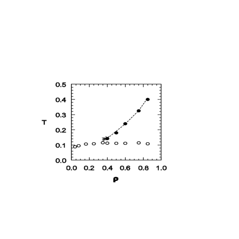
Figure 5: Loci of specific heat maxima (open and filled circles: $L=16$; crosses: $L=20$). The dashed line denotes the position of the maximum of $|d\phi/dT|$.

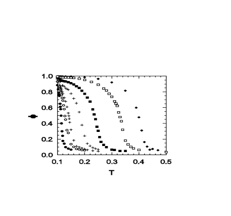
Figure 6: Order parameter versus temperature for densities (left to right) 0.25, 0.35, 0.4, 0.5, 0.6, 0.75, and 0.85.

Figure 3 shows the energy and Figure 4 the specific heat versus temperature for a number of different densities. All the specific heat curves show a peak at a temperature $T_{1}$ that increases with density for small densities, and then seems to saturate at around $T=0.11$ for $\rho\geq 0.35$. The height of this peak decreases rapidly with increasing density. For densities $\geq 0.4$, there is a second peak, at a temperature $T_{N}>T_{1}$, which increases roughly linearly with $\rho$. The locations of the specific heat peaks in the $\rho$-$T$ plane are shown in Figure 5; these loci appear to delineate a Neel line and a coexistence curve. We examine their interpretation in what follows.

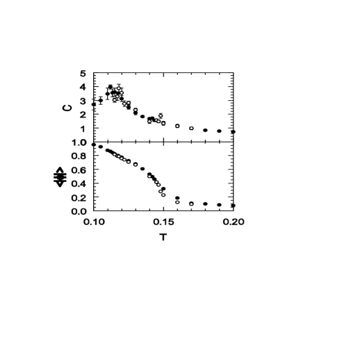
Figure 7: Upper graph: specific heat, $\rho=0.4$. Filled circles: $L=16$; open circles: $L=20$. Lower graph: order parameter for $\rho=0.4$; symbols as in upper graph.

It is tempting to associate the high-temperature specific heat peak with the onset of global sublattice ordering. Studies of the order parameter and of the charge-charge correlation function support this interpretation. In Figure 6 we plot the mean value of $|\phi|$ versus temperature for various densities. In the thermodynamic limit, this quantity should be strictly zero in the disordered phase, and should increase continuously as $T$ is reduced below $T_{N}$. Here, of course, we must anticipate finite-size rounding of the critical singularity, if any exists. The data nevertheless give strong support for $T_{N}$ marking an order-disorder transition. In fact the temperature at which $|d\phi/dT|$ takes its maximum value falls very close to that of the specific heat maximum, as shown in Figure 5.

Further support is provided by the comparison between two system sizes (for the same density, $\rho=0.4$) shown in Figure 7: the larger system presents a sharper variation in $|\phi|$ in the vicinty of the apparent transition. The high-$T$ specific heat peak, barely visible in the $L=16$ data, is quite prominent for $L=20$; both peaks shift to slightly higher temperatures for $L=20$. All of this is consistent with the system exhibiting phase transitions at $T_{1}$ and $T_{N}$. We shall therefore refer to the set of transitions commencing around $\rho=0.4$ as the Néel line.

Figure 8: Charge-charge radial distribution function, $\rho=0.75$, for three temperatures as indicated.

Figure 9: The data of Figure 8 plotted versus $1/r$. Lower set: $T=0.36$; middle: $T=0.35$; upper: $T=0.34$.

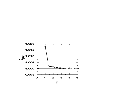
Figure 10: Density-density radial distribution function, $\rho=0.75$, $T=0.34$.

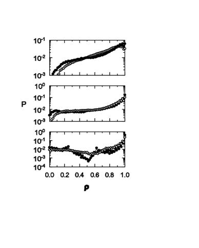
Figure 11: Cell-occupancy probabilities, $\rho=0.75$. Upper graph: open circles: $T=0.12$, filled circles $T=0.115$; middle: open, $T=0.110$, filled, $T=0.105$; lower: open, $T=0.10$, filled, $T=0.09$.

Further insight into the phase transition at or near the high-$T$ specific heat peak is afforded by the charge-charge correlation function $g_{qq}(r)$. Figure 8 shows $g_{qq}(r)$ for three temperatures in the neighborhood of $T_{N}$, for $\rho=0.75$. In all of the cases shown, $g_{qq}$ exhibits damped oscillations. At the highest temperature ($T=0.36$) the oscillations evidently decay to zero; for $T=0.35$ the decay appears to be slower, while for $T=0.34$ they seem to persist. A plot of $|g_{qq}|$ versus $1/r$ (Figure 9) yields a clearer idea of the large-$r$ behavior; from this graph it is evident that $g_{qq}$ decays to zero for $T\geq 0.35$ but not for $T=0.34$. (The specific heat peaks at $T=0.325$.) Thus the condition $lim_{r\rightarrow\infty}|g_{qq}(r)|>0$ is a criterion for the ordered phase, and the limiting value of $|g_{qq}|$ provides, in principle, an alternative definition of the order parameter. In practice, we are able to obtain $\phi$ with greater precision (smaller statistical uncertainty), and so retain it as a measure of global order.

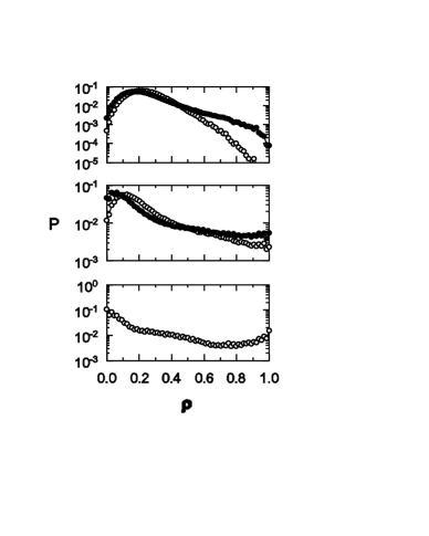
Figure 12: Cell-occupancy probabilities, $\rho=0.25$. Upper graph: open circles: $T=0.12$, filled circles $T=0.115$; middle: open, $T=0.110$, filled, $T=0.105$; lower graph: $T=0.10$.

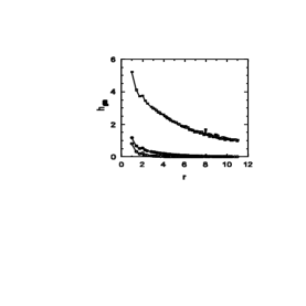
Figure 13: Density-density correlation function, $\rho=0.25$, $T=0.12$ (lower set), 0.115 (middle), and 0.11 (upper).

It is worth noting that in the neighborhood of the lambda line, the density-density correlation function $g_{\rho\rho}$ shows little structure: it has a low-amplitude peak at unit distance and then decays rapidly to its asymptotic value (see Figure 10).

We now turn to the line of low-temperature specific heat peaks. The mean-field theory results described above lead us to interpret this as a coexistence curve, so that $T_{1}(\rho)$ marks a transition from a homogeneous system to coexisting high- and low-density phases, the former disordered, the latter with sublattice ordering. To better understand what is happening at $T_{1}$, we examine the occupancy histograms. Some typical results for $\rho=0.75$ are shown in Figure 11. For $T=0.12$ the distribution is unimodal, and peaked near $\rho=0.9$. As the temperature is lowered, the distribution broadens and the peak moves to $\rho=1$ and increases in amplitude, signaling the emergence of a high-density phase. For $T=0.11$ a plateau has appeared for $0.2\leq\rho\leq 0.7$, while for $T\leq 0.10$ the distribution is bimodal. (Note also the odd-even oscillations in $P$, especially prominent for $T=0.09$. These presumably represent a tendency to local charge neutrality.) All through the transition region, the order parameter $\phi$ is very nearly unity; for this density, the transition near $T_{1}$ is not associated with the onset of sublattice order. (Such order is already present in the uniform phase for $T_{1}<T<T_{N}$.)

Figure 12 shows a series of occupancy histograms for a much lower density, $\rho=0.25$. At the highest temperature shown, $T=0.12$, the distribution peaks in the vicinity of $\rho=0.2$ and decays rapidly for higher densities. For $T=0.115$ the distribution is already considerably broader, and by $T=0.110$ a plateau near $\rho=1$ has appeared. At $T=0.105$ the distribution has become very broad, the main peak has shifted toward $\rho=0$, and a secondary peak has appeared at $\rho=1$, indicating separation into high- and low-density phases. By $T=0.10$ the transformation is complete: the histogram peaks at $\rho=0$ and $\rho=1$.

It is interesting to observe the changes in the density-density correlation function $h_{\rho\rho}(r)\equiv g_{\rho\rho}(r)-1$, in the neighborhood of the transition. In Figure 13 we see that $h$ decays rapidly for $T=0.12$ (the correlation length $\xi_{\rho}\simeq 0.9$), and is somewhat longer-ranged ($\xi_{\rho}\simeq 2.2$) for $T=0.115$. For $T=0.11$ the decay is much slower ($\xi_{\rho}\simeq 6$). At temperatures below $0.11$, the system has phase-separated and we are no longer able to infer the large-$r$ limiting value of $g_{\rho\rho}(r)$. The histogram and correlation function data suggest that for $\rho=0.25$, phase separation occurs at $T=0.105-0.110$, in agreement with transition temperature of 0.108 indicated by the specific heat maximum. In contrast to what is seen at higher densities, for $\rho=0.25$ the transition at $T_{1}$ is accompanied by the onset of sublattice order: $|\phi|$ is small for $T\geq 0.12$ and grows rapidly in the range $T=0.105$ — 0.115. This is just what one would expect, since the transition in this case marks the appearance of a high-density phase, capable of supporting NaCl-like order. (Sublattice ordering is associated with the transition at $T_{1}$ for $\rho\leq 0.25$.)

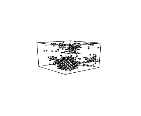
Figure 14: A typical configuration, $\rho=0.12$, $T=0.1$. Filled and empty symbols distinguish the charges.

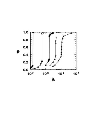
Figure 15: Density versus pair activity in in grand canonical ensemble simulations ($L=16$) for temperatures (left to right) $T=0.11$, 0.12, 0.13, 0.14 and 0.15.

Figure 14 is a snapshot of a typical configuration of the phase-separated system, in which we see a dense, crystal-like agglomerate coexisting with a dilute vapor, comprised largely of dipolar associations.

Using the specific heat data, together with results for the order parameter and the charge-charge correlation function, we have derived a series of estimates for points along the lambda line, $T_{N}(\rho)$, for $\rho=0.375$ — 0.85. The scatter amongst the values suggested by the specific heat, order parameter, and correlation function data yields an uncertainty estimate for $T_{N}(\rho)$. Similarly, we use the specific heat, cell occupancy histogram, and density-density correlation function data to estimate the phase-separation temperature $T_{1}(\rho)$.

In an effort to determine the coexisting densities with greater precision, we also performed grand canonical ensemble (GCE) simulations. Figure 15 shows the dependence of the density on the pair activity $\lambda$. For $T=0.15$ the dependence is smooth, but for $T\leq 0.14$ there is a discontinuity at $\lambda_{c}(T)$. Hysteresis effects are minimal for $T\geq 0.12$, and the coexisting densities are given by the limiting values as we approach $\lambda_{c}$ from above and below. The GCE studies furnish an independent prediction for the coexistence curve in the range $T=0.12$ — 0.14.

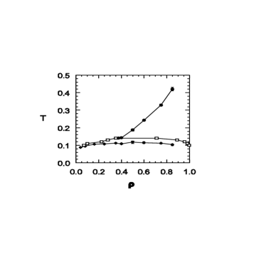
Figure 16: Best estimates for the location of the lambda line and coexistence curve. Filled symbols: canonical ensemble simulations; open symbols: GCE simulations.

In Figure 16 we plot our best estimates for $T_{N}$ (from canonical simulations), and for the coexistence curve, from both the canonical and GCE studies. Evidently, the coexistence curve is shifted upward in the GCE simulations, whose results place the tricritical point (i.e., the intersection of the lambda line and the coexistence curve), at around $T=0.14$, as opposed to about $T=0.115$ in the canonical studies. Since the two ensembles are not required to give identical results for finite systems, there is no inconsistency implied. The grand canonical results, however, seem preferable on several grounds. First, the shape of the coexistence curve looks more reasonable (more like the familiar Ising/lattice gas coexistence curve). More significantly, perhaps, the GCE curve actually meets the lambda line, which appears to veer horizontally near $\rho=0.4$, and shows no sign of ever encountering the canonical coexistence curve. Given the large surface effects implicit in phase coexistence in a small system, the GCE, which studies homogeneous phases, seems more likely to give reliable results in a finite size simulation. One may speculate that the large surface energy depresses the transition temperature in the canonical ensemble simulations. A more definitive answer to this question must await the results of larger scale simulations.

Discussion and Summary

We have determined the phase diagram of the lattice restricted primitive model in extensive Monte Carlo simulations. Our simulations reproduce the principal features expected on the basis of general arguments and mean-field theory, that is, a $\lambda$-line of Néel points meeting a coexistence curve at a tricritcal point. Our best estimate for the location of the tricritical point is $T_{t}\simeq 0.14$, $\rho_{t}\simeq 0.4$, while mean-field theory predicts $T_{t}=0.299$ and $\rho_{t}=1/3$. This comparison is consistent with the tendency of mean-field theories to overestimate transition temperatures, and underestimate transition densities (i.e., to overestimate the stability of ordered phases).

During the completion of this work we learned of Panagiotopoulos and Kumar’s simulation results for the LRPM panag , which include a study of the effects of varying the size of the hard core. Their results for the case of site-exclusion studied here support our conclusions for the phase diagram, with the exception that the tricritical density is somewhat larger ($\rho_{t}\simeq 0.48$ in their work) and the Néel line appears to be nearly vertical in the vicinity of the tricritical point.

Because our results come almost entirely from studies of a single system size ($L=16$), it is difficult to assign meaningful uncertainties to $T_{t}$, $\rho_{t}$, or, indeed, the location of the $\lambda$-line in the $\rho$-$T$ plane. The limited comparison we made with a system of size $L=20$ (Figure 7) suggests that the true transition temperature (for the $\lambda$-transition) may be 5—10% higher than that observed for $L=16$. We have also noted a sizeable discrepancy ($\approx 25$%) between canonical and grand canonical simulations regarding the position of the coexistence curve along the $T$-axis. Studying larger systems is therefore the first order of business for future simulations of the LRPM. Since simulations are quite slow, with many trial moves rejected at the low temperatures of interest, even for the relatively small systems studied here, we anticipate the need for non-Metropolis simulation methods utilizing histograms, multi-canonical sampling, and/or cluster dynamics to augment efficiency.

If such methods can be developed, a number of issues can be explored. It is of interest to understand the nature of the transitions occuring along the $\lambda$-line and at the tricritical point, to assign these their proper universality classes. We may also anticipate that the interface between the dense and dilute phases undergoes a roughening transition at a certain temperature. Another topic worthy of investigation is the global phase diagram as one goes from the Coulombic system studied here to a lattice gas with nearest-neighbor interactions, via a family of models described by a potential (e.g., of Yukawa form) having a range parameter. The LRPM with a lattice Green’s function interaction, and on lattices that do not support antiferromagnetic order, are, as noted above, further topics for future work.

References

- (1) Debye, P. P., and Hückel, F., Phys. Z. 24, 185 (1923).
- (2) Stell, G., Wu, K. C., and Larsen, B., Phys. Rev. Lett. 37, 1369 (1976).
- (3) Orkoulas, G., and Panagiotopoulos, A. Z., J. Chem. Phys. 101, 1452 (1994).
- (4) Caillol, J. M., Levesque, D., and Weis, J. J., J. Chem. Phys. 107, 1565 (1997).
- (5) Valleau, J.-P., and Torrie, G., J. Chem. Phys. 108, 5169 (1998).
- (6) Stell, G., Phys. Rev. A 45, 7628 (1992).
- (7) Stell, G., J. Stat. Phys. 78, 197 (1995).
- (8) Blume, M., Phys. Rev. 141, 517 (1966).
- (9) Capel, H. W., Physica 32, 966 (1966).
- (10) McCoy, B., and Wu, T. T., The Two-Dimensional Ising Model, Cambridge, Mass.: Harvard University Press, 1973.
- (11) Baxter, R. J., Exactly Solved Models in Statistical Mechanics, New York: Academic Press, 1982.
- (12) Stell, G., “New Results on Some Ionic-Fluid Problems,” in New Approaches to Problems in Liquid State Theory, Caccamo, C., Hansen, J.-P., and Stell, G., eds., Dordrecht: Kluiver Academic Publishers, 1999.
- (13) Høye, J. S., and Stell, G., J. Stat. Phys. 89, 177 (1997).
- (14) Ciach, A., and Stell, G., J. Mol. Loquids, to appear; preprint, 1999.
- (15) Frölich, J., Israel, R., Lieb, E., and Simon, B., J. Stat. Phys. 22, 296 (1980).
- (16) Tosi, M. P., Solid State Physics, vol. 16, Seitz, F., and Turnbull, D., eds., New York: Academic Press, 1964.
- (17) Ladd, A. J. C., Molec. Phys. 33, 1079 (1997); ibid., 38, 463 (1978).
- (18) de Leeuw, S. W., Perram, J. W., and Smith, E. R., Proc. R. Soc. Lond. A 373, 27 (1980).
- (19) Panagiotopoulos, A. Z., and Kumar, S. K., preprint, 1999.