Evidence of exactness of the mean field theory in the nonextensive regime of long-range spin models
Abstract
The -state Potts model with long-range interactions that decay as subjected to an uniform magnetic field on –dimensional lattices is analized for different values of in the nonextensive regime . We also consider the two dimensional antiferromagnetic Ising model with the same type of interactions. The mean field solution and Monte Carlo calculations for the equations of state for these models are compared. We show that, using a derived scaling which properly describes the nonextensive thermodynamic behaviour, both types of calculations show an excellent agreement in all the cases here considered, except for . These results allow us to extend to nonextensive magnetic models with a previous conjecture which states that the mean field theory is exact for the Ising one.
pacs:
05.50.+q;75.10.Hk;05.70.CeI Introduction
Microscopic pair interactions that decay slowly with the distance between particles appear in different physical systems. Typical examples are gravitational and Coulomb interactions, where the potential decays as . Several other important examples can be found in condensed matter, such as dipolar (both electric and magnetic) and Ruderman-Kittel-Kasuya-Yosida (RKKY) interactions, both proportional to . Effective interactions with a power law decay , with some exponent , appear also in other related problems such as critical phenomena in highly ionic systems[3], Casimir forces between inert uncharged particles immersed in a fluid near the critical point[4] and phase segregation in model alloys[5].
It is known that some of these systems can exhibit nonextensive thermodynamic behaviour (see Refs.[6, 7] and references therein). In other words, for small enough values of the ratio the free energy , with ( being the Hamiltonian of the system, the dimensionality and ), grows faster than the number of microscopic elements when , and the thermodynamic limit is not well defined.
In a recent communication[7] two of us analized the thermodynamics associated with the long range (LR) ferromagnetic Ising Hamiltonian
| (1) |
with
| (2) |
where is the distance (in crystal units) between sites and , and where the sum runs over all distinct pairs of sites on a -dimensional hypercubic lattice. It was shown[7] that the quantities per particle: free energy , internal energy , entropy and magnetization of a finite model of spins behave according to Tsallis conjecture[8] for . These quantities present, in the presence of an external magnetic field , the following asymptotic scaling behaviours:
| (3) | |||||
| (4) | |||||
| (5) | |||||
| (6) |
for all , where the functions , , and are the corresponding quantities associated with the same model but with rescaled coupling (these functions are independent of the system size ) and the function is defined as
| (7) |
which behaves, for , as
| (8) |
For the thermodynamic functions per site do not depend on and the system is extensive (i.e., the thermodynamic limit exists). When , diverges for and the system is non-extensive. It was also presented numerical evidence[7] that for the mean field (MF) theory becomes exact when . This led two of us to conjecture that the mean field theory might be exact for the nonextensive Ising model.
In this work we extend the previous analysis and present new evidences of the exactness of the MF theory for for the one dimensional ferromagnetic -state LR Potts model for different values of (including the first order phase transition predicted by MF theory for ) and also for the two- dimensional antiferromagnetic LR Ising model in an external field.We, thus, conjecture that the MF theory might be exact for any nonextensive magnetic model excluding the borderline case , where there are probably corrections to the MF results (some previous experimental results [9] on dipolar ferromagnetic materials do not exclude this possibility).
The outline of this paper is the following. In section II we analize the ferromagnetic q–state LR Potts model subjected to an uniform magnetic field . First, we show that the previous analysis for the Ising model () in the non-extensive region is straightforwardly extended to the generic case. Then, in subsection II-A we derive the mean field solution of this model for arbitrary values of , and , in particular the MF predictions for the LR bond percolation which corresponds to the and limit. In subsection II-B we compare the MF solution with our Monte Carlo simulation of the one-dimensional model for , and and different values of . In section III we calculate the mean field solution of the two-dimensional Ising model with competing LR antiferromagnetic and short-range ferromagnetic interactions in an external field and compare them with the Monte Carlo results of Sampaio et al[10]. Some comments and conclusions are presented in section IV.
II Potts model with long-range ferromagnetic interactions
In this section we address the LR ferromagnetic state Potts model, i.e., we consider the Hamiltonian:
| (9) |
where to each site, , we associate a spin variable , which can assume integer values; the sum runs over all distinct pairs of sites of a -dimensional lattice of sites (); is the Kronecker delta function, is given by Eq.(2) and is an external magnetic field in the direction. The limit corresponds to the first-neighbor model. For the limit corresponds, after a rescaling , to the Curie-Weiss model.
This model, in its plain formulation ( of Eq.(9)) or in a more general one with many-body interactions, is at the heart of a complex network of relations between geometrical and/or thermal statistical models, like for example various types of percolation, vertex models, generalized resistor and diode network problems, classical spin models, etc (see [11] and references therein).
On the other hand, the Potts model with LR interactions has been much less studied. In the extensive regime it presents a very rich thermodynamic behaviour, even in the one-dimensional case[12, 13, 14]. To the best of our knowledge, no study has been carried out for the nonextensive regime .
Let us introduce the sums . A sufficient condition (and believed to be necessary[15, 16]) for the existence of the thermodynamic limit of this system is that
| (10) |
Let us now consider a d-dimensional hypercube of side and , and let be the central site of the hypercube. We have that
| (11) |
When () shows the following asymptotic behaviour[7]:
| (12) |
where is given by Eq.(7) and is a continuous function[7] of independent of , with . It can be proved that[7]:
| (13) |
where is the Riemann Zeta function. From Eqs.(7)–(12) we see that the thermodynamic limit is well defined for (where the system presents extensive behaviour), while for the system becomes non-extensive. Following the same procedure as in Ref.[7] it can be shown that the scaling behaviours (3)-(6) of the thermodynamic functions hold and . For the system undergoes a second order phase transition at finite temperature for all when [17] and for when [18]. For , the critical temperature shows the following asymptotic behaviour [17]:
| (14) |
For and (short-range case[11]) there exists a critical value such that the phase transition is a second order one when ( for ) and a first order one for . For and Monte Carlo simulations[14] show that, for , there is a q-dependent threshold value such that the transition is of first order when and of second order above it.
A Mean field theory
In order to develop a mean field version of Hamiltonian (9) we use Mittag and Stephen[19] spin representation for the Potts model, i.e., we associate to each site a spin variable which can take the values , where is a th root of unity. In other words, if the site is in the state then . Then, using the property
| (15) |
we can rewrite the Hamiltonian (9) as:
| (16) |
where the constant term is
| (17) |
The fraction of sites in the state , , in this representation is given by:
| (18) |
and the order parameter for a symmetry breaking in the direction is
| (19) |
which can be written, using Eq.(18), as:
| (20) |
The mean field solution for this model can be easily found from the Variational Method in Statistical Mechanics[20] by using a non–interacting trial Hamiltonian given by
| (21) |
where is the variational parameter to be found as a function of temperature. The variational free energy is given by
| (22) | |||||
| (23) |
where the free energy associated with is
| (24) |
and denotes the canonical average using the Boltzmann measure proportional to .
Using equality (15) one gets that
| (25) |
where the variational order parameter (defined by an equation similar to Eq.(20)) is related to through:
| (26) |
and from the property it follows that
| (27) |
The minimization condition leads to
| (28) |
which, combined with Eq.(26) gives the following mean field equation for the order parameter :
| (29) |
In the limit (short range interactions) we have , being the coordination number of the lattice, and we recover,for , Mittag and Stephen’s [19] result. For the Hamiltonian (9) is equivalent to the Ising one with long range interactions, providing that and . In this case Eq.(29) reduces to
| (30) |
and we recover the result from Ref.[7], i.e., the long range version of the Curie-Weiss equation which describes a second order phase transition for at .
The variational free energy calculated at the minimum (condition (28)) gives the following mean field free energy per site :
| (32) | |||||
For and the transition is of first order and it is easy to verify from Eq.(32) that at the critical temperature the order parameter jumps from zero to the value . The critical temperature for is given by
| (33) |
which recovers, in the limit, Mittag and Stephen’s result[19].
In the limit, which corresponds to a bond percolation where the bond probability occupancy between any two sites and is , the order parameter probability percolation (defined as the probability that a randomly chosen bond of an infinite lattice belongs to a cluster of infinite size) can be derived from[21]
| (34) |
where , is the partition function of the Potts model with coupling constants and is the first neighbor bond probability given by .
One can easily show, from Eqs. (29), (32) and (34), that the probability percolation is, as expected[16], exactly the and limit of the order parameter , namely,
| (35) |
or, in terms of ,
| (36) |
from which it follows that, due to the divergence of in the non–extensive regime, and, hence, the critical probability in agreement with the exact result[16].
One can easily prove, from Eq.(36), that the percolation probability of a finite system with bonds presents an asymptotic scaling behavior similar to Eq.(6), namely
| (37) |
where is the variable calculated at , namely,
| (38) |
and is the probability percolation associated with the long range bond percolation whose bond probability occupancies are . Using this rescaled variable , the MF order parameter equation becomes, for (see Eq.(12)):
| (39) |
which leads, for different values of , to monotonously increasing distinct order parameters as varies from the critical probabilites to . However, if one introduces a more convenient variable, namely,
| (40) |
then all these MF probability percolation curves for different values of and coalesce into a single curve described by the equation
| (41) |
The critical value where vanishes is , which leads to the MF critical probability
| (42) |
| (43) |
which, in the particular case of , gives
| (44) |
—————
B Monte Carlo results
We performed a Monte Carlo simulation using the heat bath algorithm on the one-dimensional Hamiltonian (9) with and periodic boundary conditions for , and , for , and , and different values of . We calculated the magnetization per spin (19) as a function of for different system sizes and performed a numerical extrapolation for .
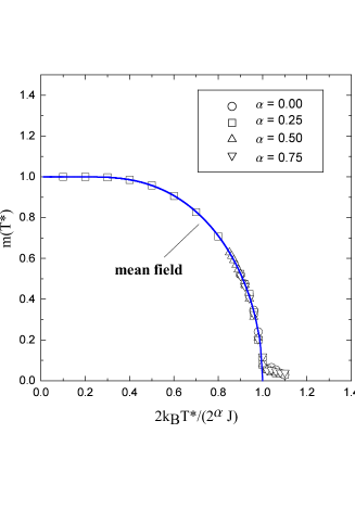
In Fig. 1 we compare the numerical results of the case for vs. for different values of with the mean field solution (equation (30)). We see that all the numerical curves fall into a single one in excelent agreement with the MF prediction.

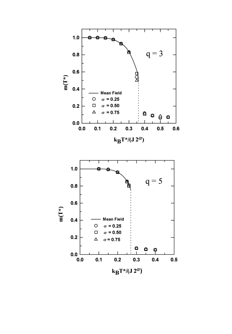
In Fig. 2 we make the same comparison for the and cases. The solid lines represent the MF solution given by equation (29) for . The dotted lines in this figure indicate the mean field prediction for the critical temperature jumps (33). Again we observe, in both cases, an excelent agreement between our simulations and MF results for , including the first order phase transition for .

III Antiferromagnetic Ising model with long-range interactions
We now consider an Ising model with competing LR antiferromagnetic and short-range ferromagnetic interactions in an external field, which is described by the Hamiltonian:
| (45) |
where , and the sum runs over nearest-neighbor sites of a d-dimensional hypercubic lattice. The above Hamiltonian reduces, for and , to the model studied by Sampaio et al [10] through Monte Carlo simulations.
A mean field version of this model can be obtained by considering the Hamiltonian
| (46) |
with
| (47) |
where the sum runs over all nearest-neighbor sites of and
| (48) |
with
| (49) |
Now we consider the particular case of a square lattice. Dividing our lattice into two square interpenetrated sublattices A and B we can propose a solution of the form:
| (50) |
Let us introduce the functions
| (51) | |||||
| (52) |
with
It can be easily seen that
| (53) | |||||
| (54) |
| (55) |
Combining Eqs.(55), Eq.(46) and Eq.(48) we arrive, after some algebra, to the following set of MF equations for the magnetization and for the staggered magnetization :
| (56) |
| (57) |
| (58) |
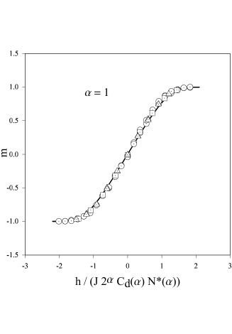
In figure 3 we compare a numerical solution of Eq.(58) with the Monte Carlo data of Sampaio et al[10] for , , , and different values of . The function for was evaluated numerically. We obtained, for , . The comparison for other values of gave similar results.

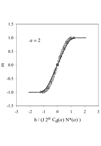
A similar comparison for is made in figure 4 (). The Monte Carlo data of Sampaio et al[10] do not agree very well with the MF magnetization, suggesting that corrections to the mean field result should be taken into consideration in this borderline case (where ). Notice that theoretical [23] predictions and experimental results [9] obtained for the critical behavior of uniaxial ferromagnets with exchange and strong dipolar interactions show that corrections to the MF behavior are needed in this case.
Summarizing this section, we verify that the Monte Carlo simulations for the equation of state of the LR Ising antiferromagnet are in excellent agreement with the MF prediction when .

IV Conclusions
We have analyzed, in this paper, two long range spin models with power law decaying interactions () under an uniform magnetic field : (i) the -state LR Potts ferromagnet on d-dimensional hypercubic lattices (including the and case of LR bond percolation) and (ii) the LR square Ising antiferromagnet with first-neighbor ferromagnetic interactions. Both models present non-extensive thermodynamic behaviors when , but their thermodynamic functions become finite when conveniently scaled variables are used [8]. We have derived this scaling for and have shown that the mean field probability percolation (i.e. the percolation order parameter) satisfies a similar scaling. The derived MF solution for the free energy of the LR Potts model led to spontaneous magnetization curves which agree very well with our Monte Carlo simulations for and , and states for different values of . An excellent agreement occurred also between the derived MF equation of state for the above antiferromagnetic LR model and the Monte Carlo simulations of Sampaio et al [10] for distinct values of . Our results strongly suggest that the mean field theory is exact for LR non-extensive spin models with . This conjecture is also supported by the fact that Bergersen et al [24] Monte Carlo simulations of the correlation function of the LR d=1 Ising ferromagnet reproduce the MF result when . Since our conjecture predicts, for the LR Potts ferromagnet, a first order transition for and , it matches nicely with previous results [14] exhibiting first order transition for .
Our results show that mean field behaviour is robust against variations of the range of interactions within the non-extensive region, for a large class of magnetic systems. If our conjecture were true, this would have important practical implications: if you are considering systems with slow enough decaying interactions then you do not need sophsiticated approximations.
It would be very interesting to extend the present analyis to more general non-extensive systems of interacting particles with long-range interactions.
V Acknowledgments
Fruitful discussions with Z. Glumac, C. Tsallis and E.M.F.Curado are acknowledged. We are greatful to Sampaio and colaborators for sending us their Monte Carlo data. This work was partially supported by grants from Consejo Nacional de Investigaciones Científicas y Técnicas CONICET (Argentina), Consejo Provincial de Investigaciones Científicas y Tecnológicas (Córdoba, Argentina) and Secretaría de Ciencia y Tecnología de la Universidad Nacional de Córdoba (Argentina), Conselho Nacional de Desenvolvimento Científico e Tecnológico (CNPq) and PRONEX/FINEP/MCT.
REFERENCES
- [1] E-mails: cannas@fis.uncor.edu, aglae@cbpf.br and tamarit@fis.uncor.edu
- [2] Members of the National Research Council, CONICET (Argentina)
- [3] K. S. Pitzer, M. C. P. de Lima and D. R. Schreiber, J. Phys. Chem. 89, 1854 (1985).
- [4] T. W. Burkhardt and E. Eisenriegler, Phys. Rev. Lett. 74, 3189 (1995).
- [5] G. Giacomin and J. L. Lebowitz, Phys. Rev. Lett. 76, 1094 (1996).
- [6] N. Goldenfeld, Lectures on Phase Transitions and the Renormalization Group, (Addison Wesley, 1992).
- [7] S. A. Cannas and F. A. Tamarit, Phys. Rev. B 54, R12661(1996).
- [8] C. Tsallis, Fractals 3, 541 (1995).
- [9] J. Als-Nielsen, L. M. Holmes and H. J. Guggenheim, Phys. Rev. Lett. 32, 610 (1974); G. Alhers, A. Kornblit and H.J. Guggenheim, Phys. Rev. Lett. 34, 1227 (1975); A. Kornblit and G. Alhers, Phys. Rev. B* 11, 2678 (1975).
- [10] L.C. Sampaio, M.P. de Albuquerque and F.S. de Menezes, Phys. Rev. B55, 5611 (1997).
- [11] C. Tsallis and A. C. N. de Magalhães, Phys. Rep. 268, 305 (1996).
- [12] S. A. Cannas and A. C. N. de Magalhães, J. Phys. A: Math. and Gen. 30, 3345 (1997).
- [13] Z. Glumac and K. Uzelac, J. Phys. A: Math. and Gen. 26, 5267 (1993).
- [14] K. Uzelac and Z. Glumac, Fizika B6, 133 (1997); Z. Glumac and K. Uzelac, Phys. Rev. E 58, 4372 (1998).
- [15] C. J. Thompson, Classical Equilibrium Statistical Mechanics, (Clarendon Press - Oxford, 1988).
- [16] M. Aizenman, J. T. Chayes, L. Chayes and C. M. Newman, J. Stat. Phys. 50, 1 (1988).
- [17] B. J. Hiley and G. S. Joyce, Proc. Phys. Soc. 85, 493 (1965).
- [18] F.J. Dyson, Commun. Math. Phys. 12, 91 (1969); F.J. Dyson, Commun. Math. Phys. 12, 212 (1969); J. Frölich and T. Spencer, Commun. Math. Phys. 84, 87 (1982); Z. Glumac and K. Uzelac, J. Phys. A: Math, and Gen. 22, 4439 (1989); S.A. Cannas, Phys. Rev. B 52, 3034 (1995).
- [19] L. Mittag and M. J. Stephen, J. Phys. A.: Math., Nucl, Gen., 9, L109 (1974).
- [20] K. Huang, Statistical Mechanics, J. Wiley (1963), chapter X, section 10.3.
- [21] P.W. Kasteleyn and C.M. Fortuin, J. Phys. Soc. Jap., Suppl. 26, 11 (1969); F.Y. Wu, J. Stat. Phys. 18, 115 (1978).
- [22] L.S. Schulman, J. Phys. A: Math. and Gen. 16, L639 (1983).
- [23] A.I. Larkin and D.E. khmel’nitskii, Zh. Eksp. Teor. Fiz. 56, 2087 (1969) [ Sov. Phys.-JETP29, 1123 (1969)]*; A. Aharony, Phys. Rev. B 8, 3363 (1973).
- [24] B. Bergersen, Z. Racz and H-J. Xu, Phys. Rev. E 52, 6031 (1995).